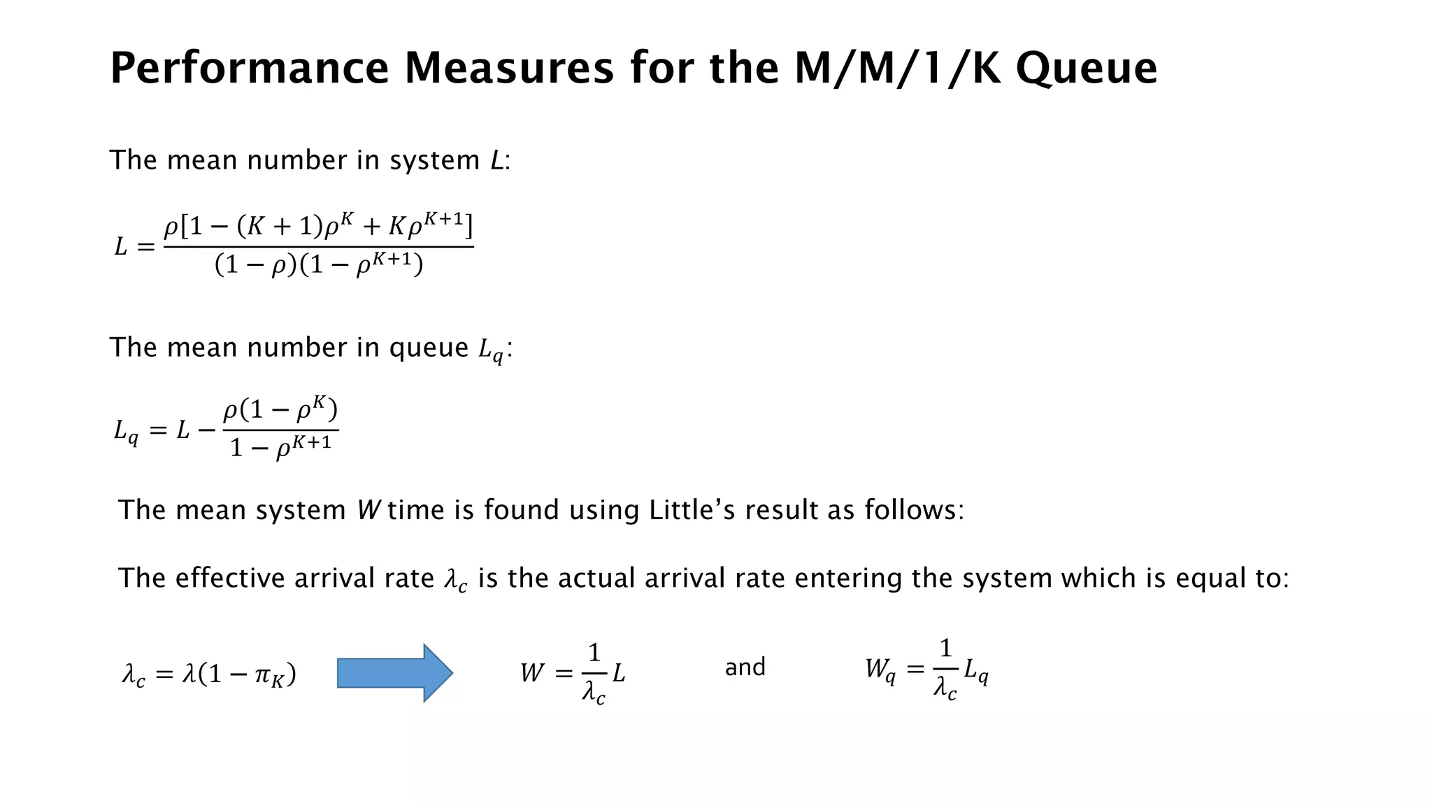
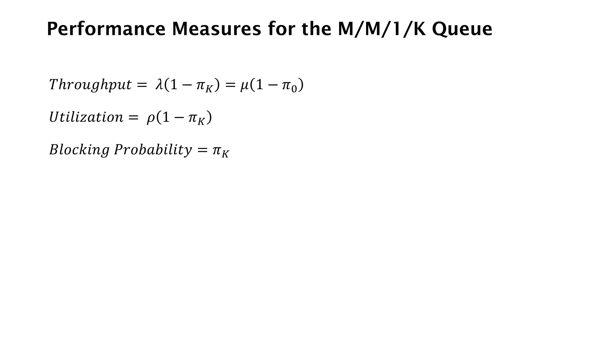
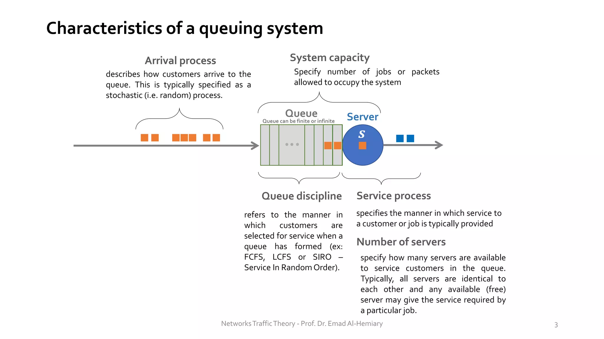
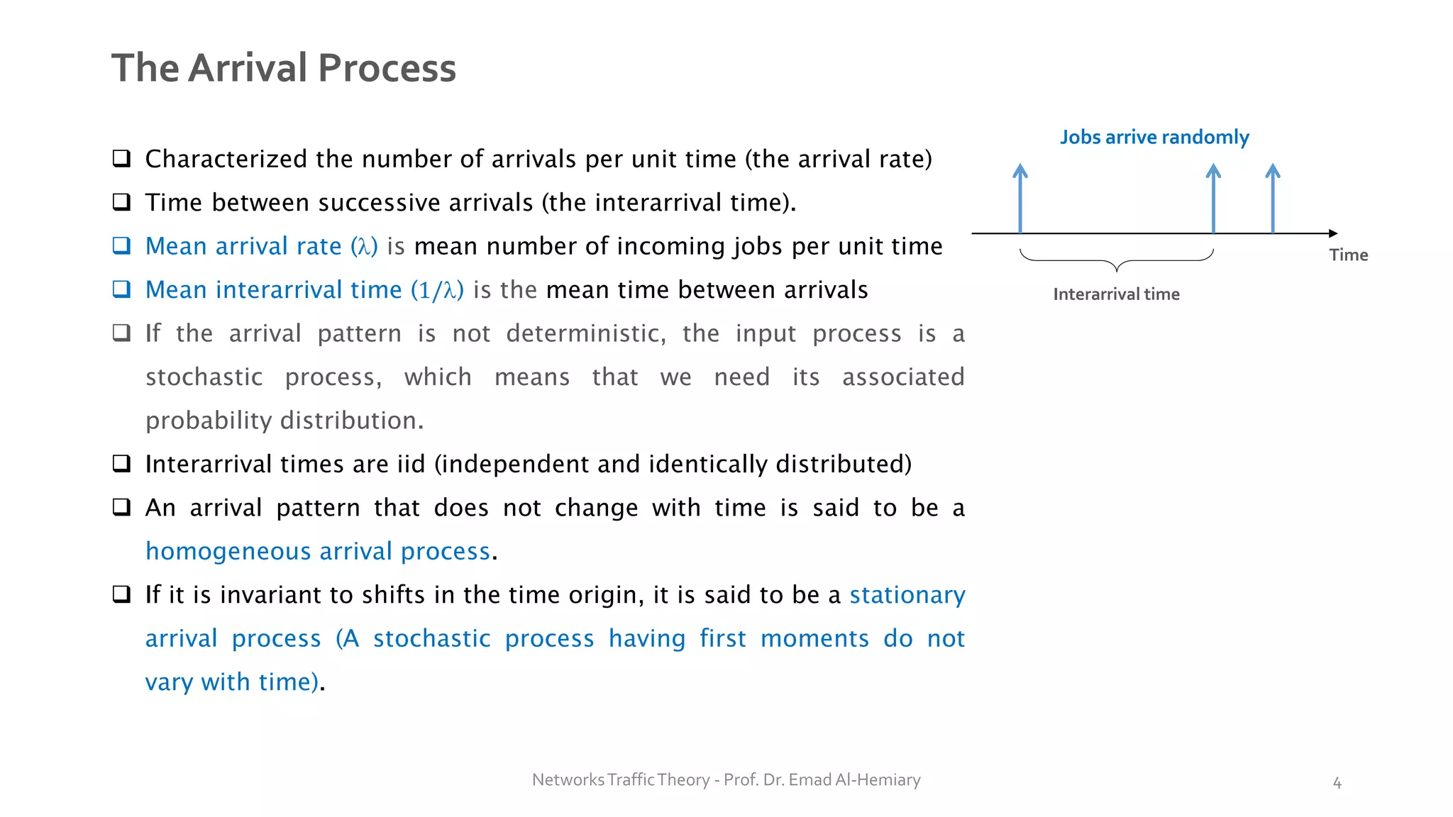
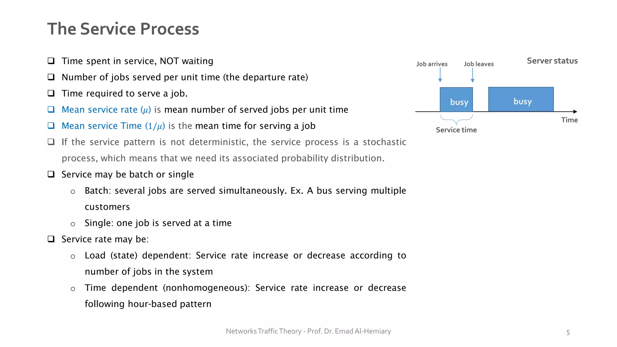
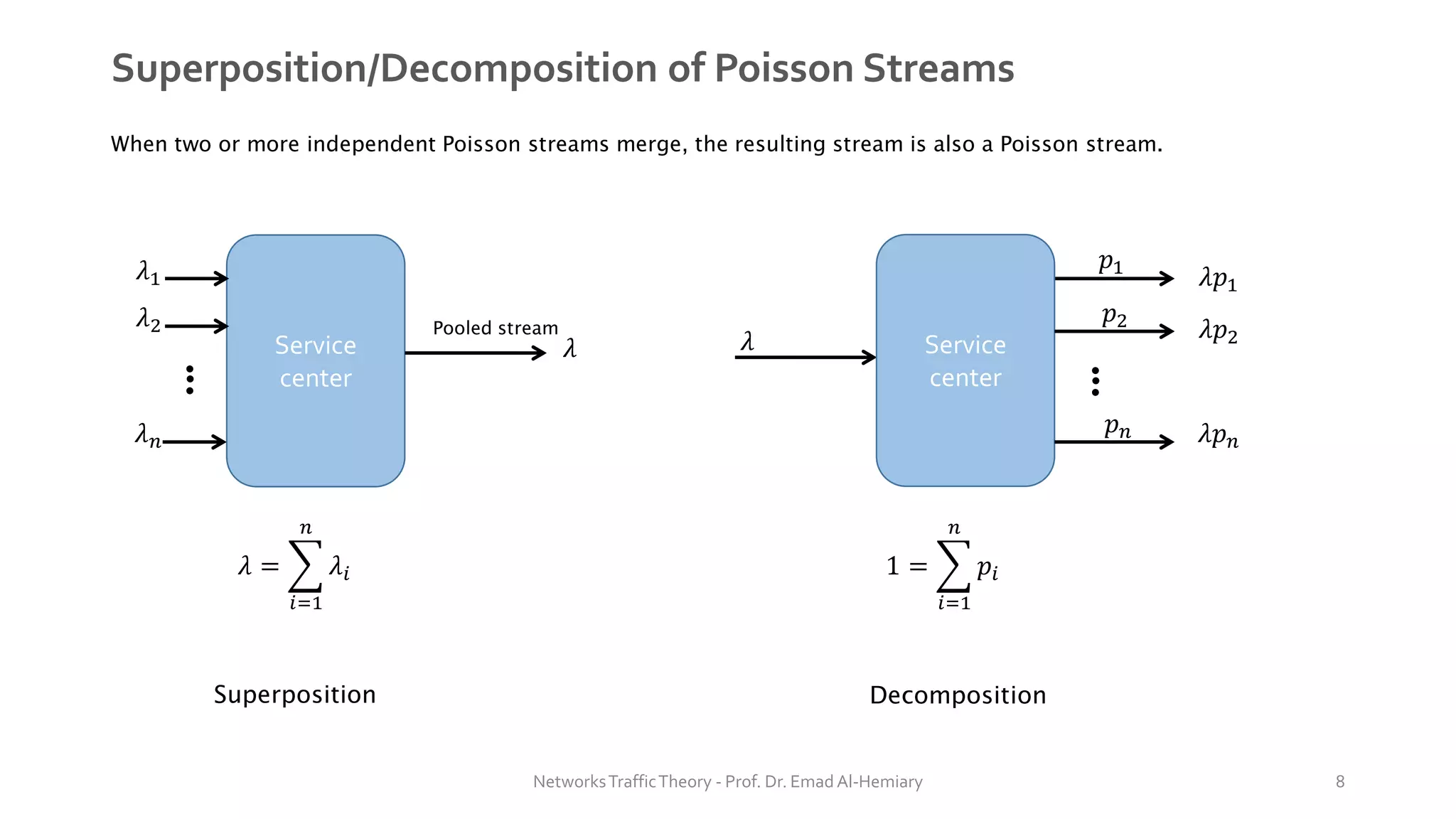
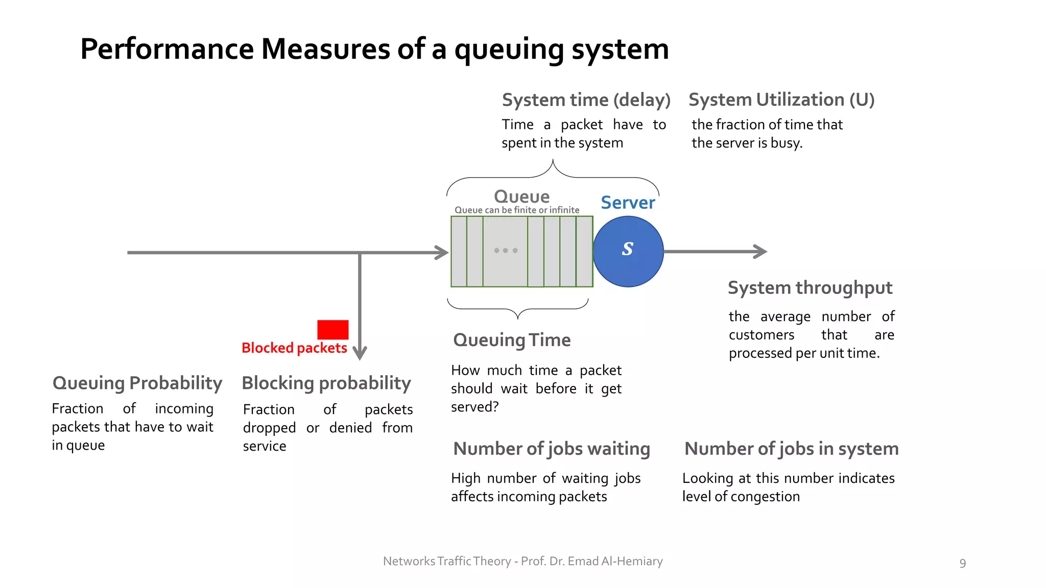
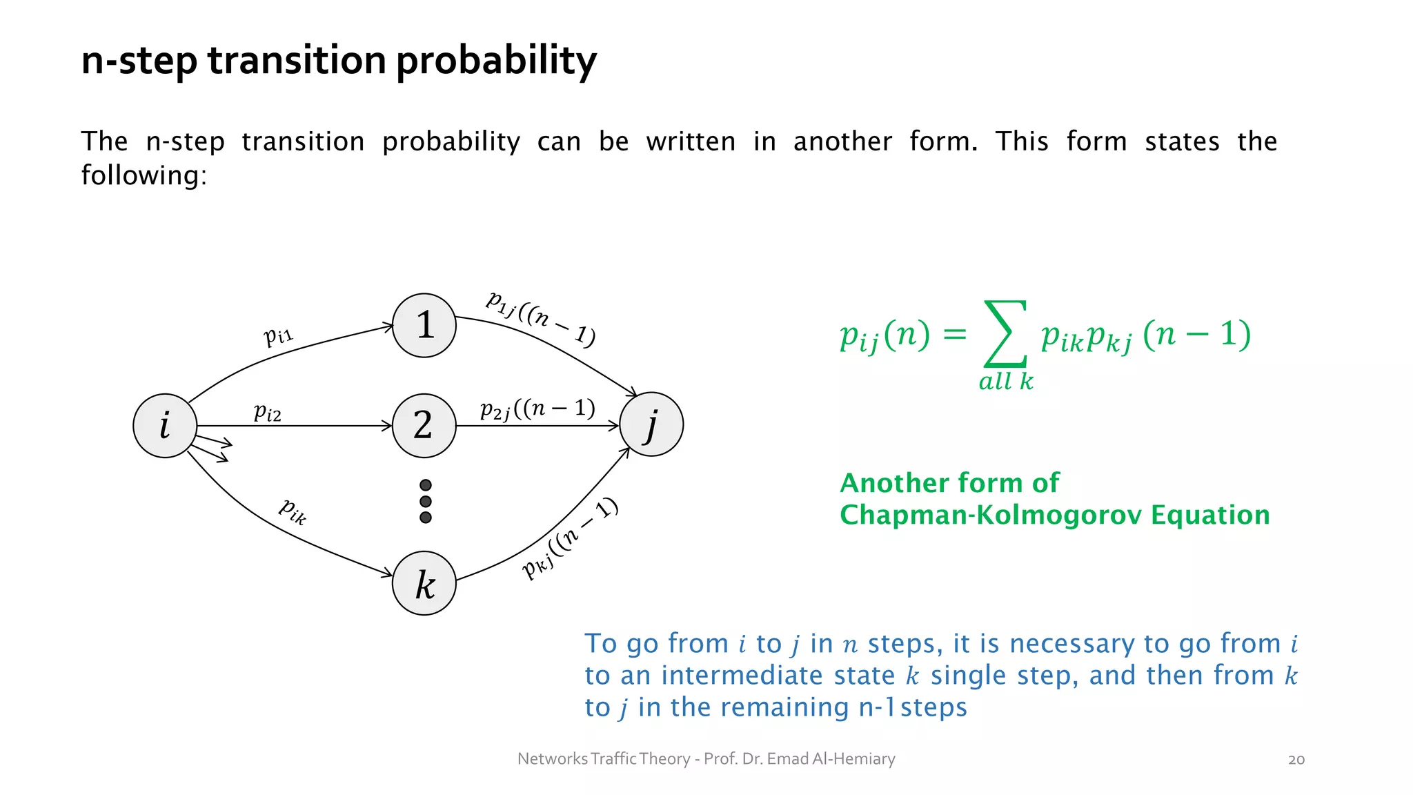
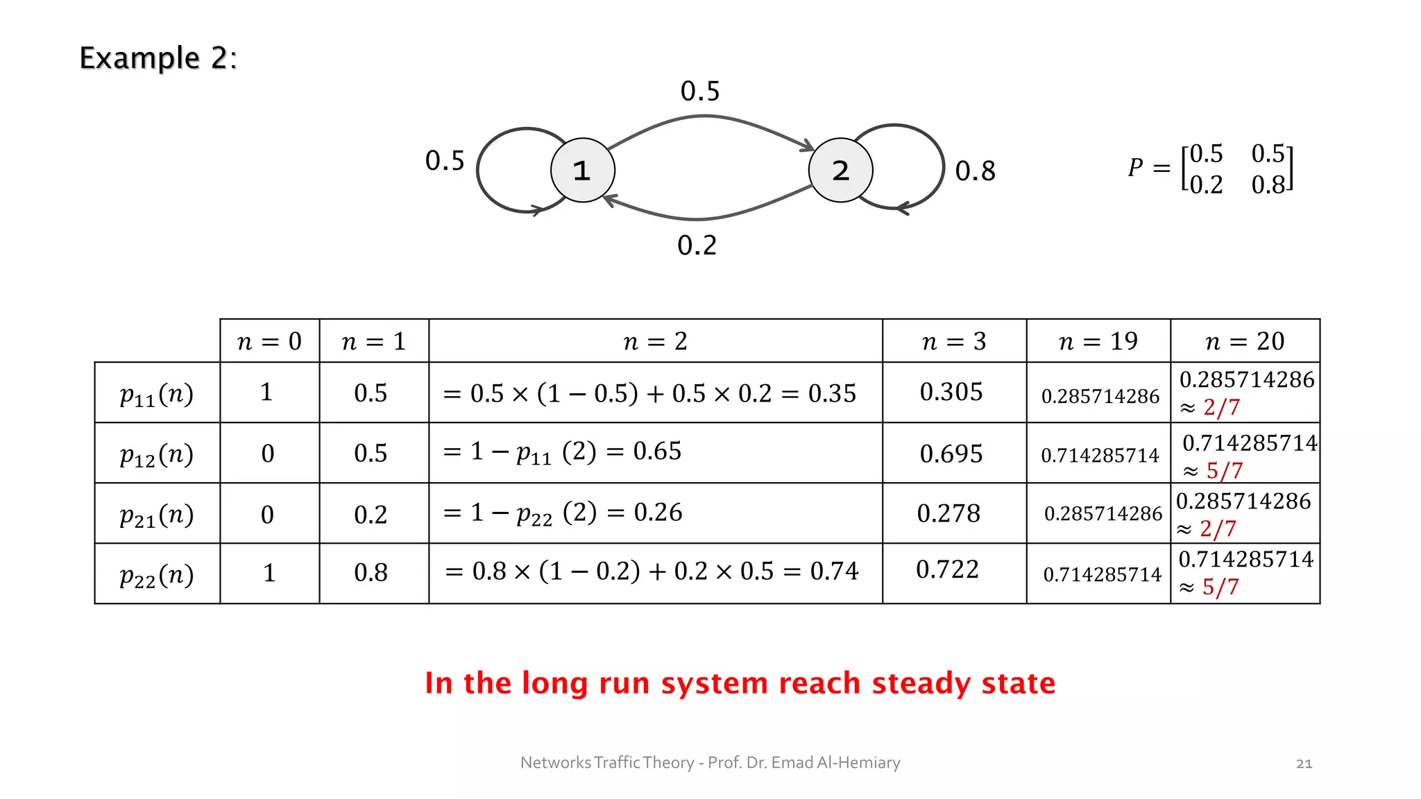
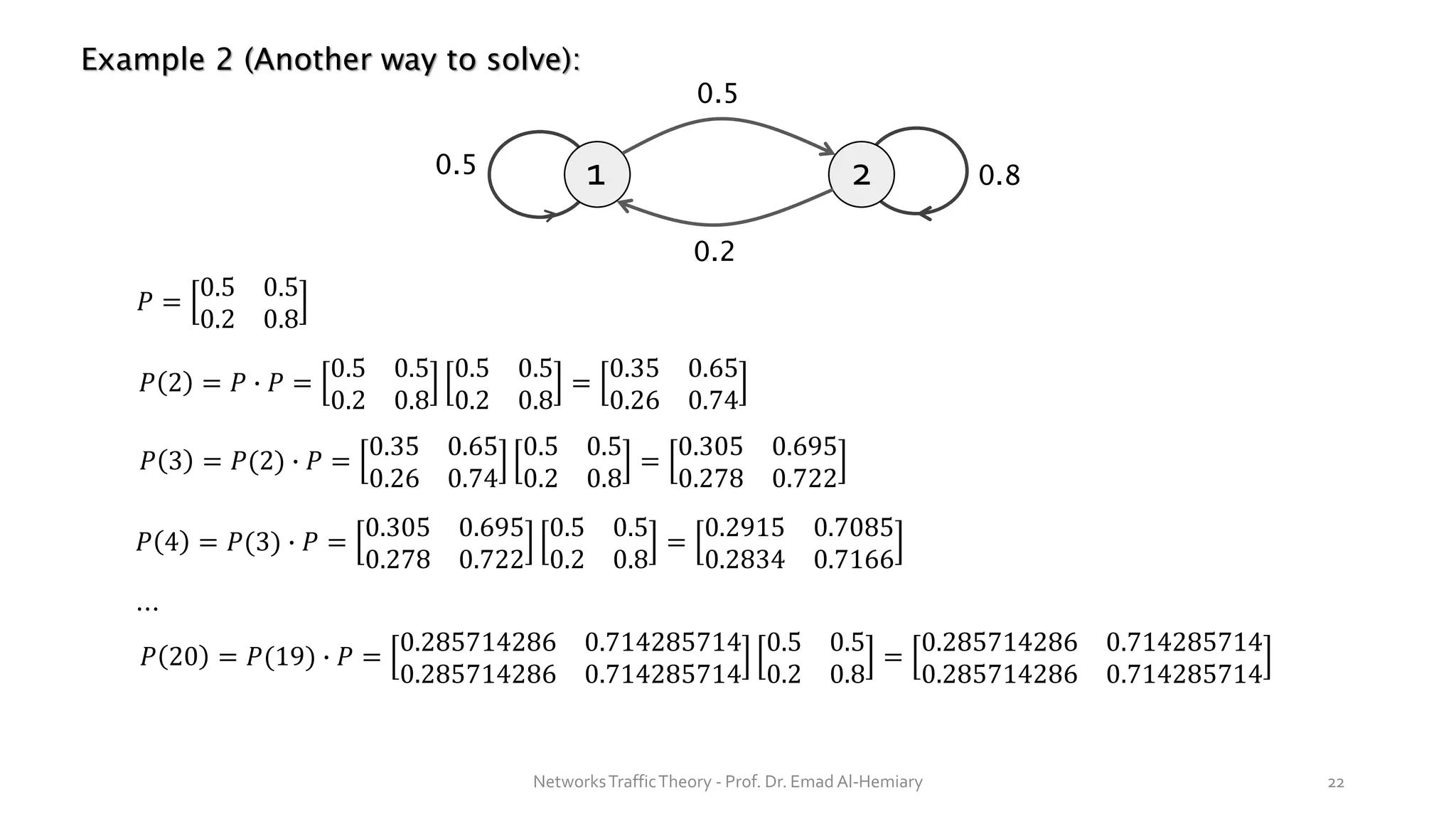
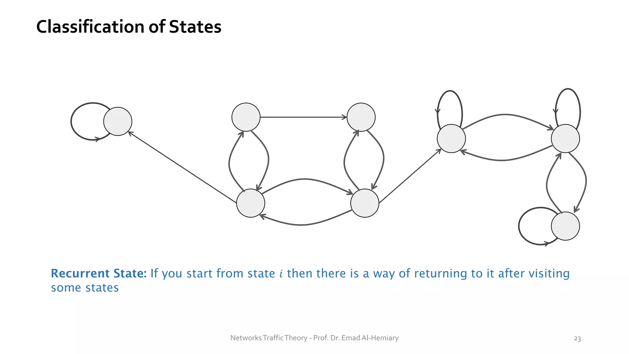
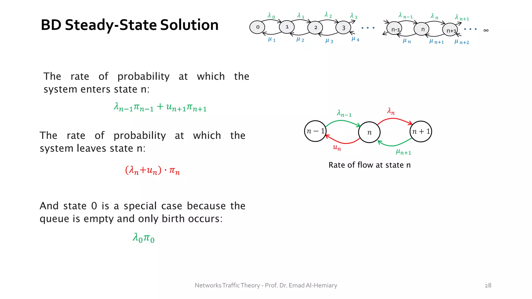
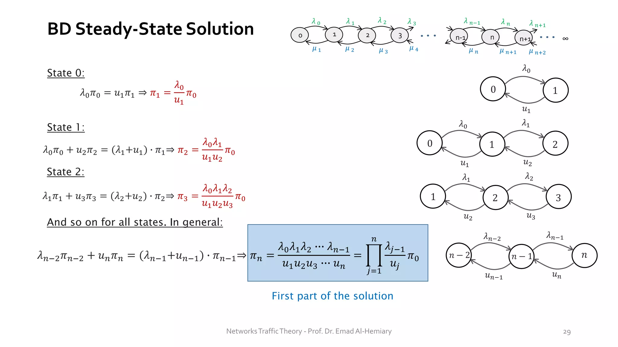
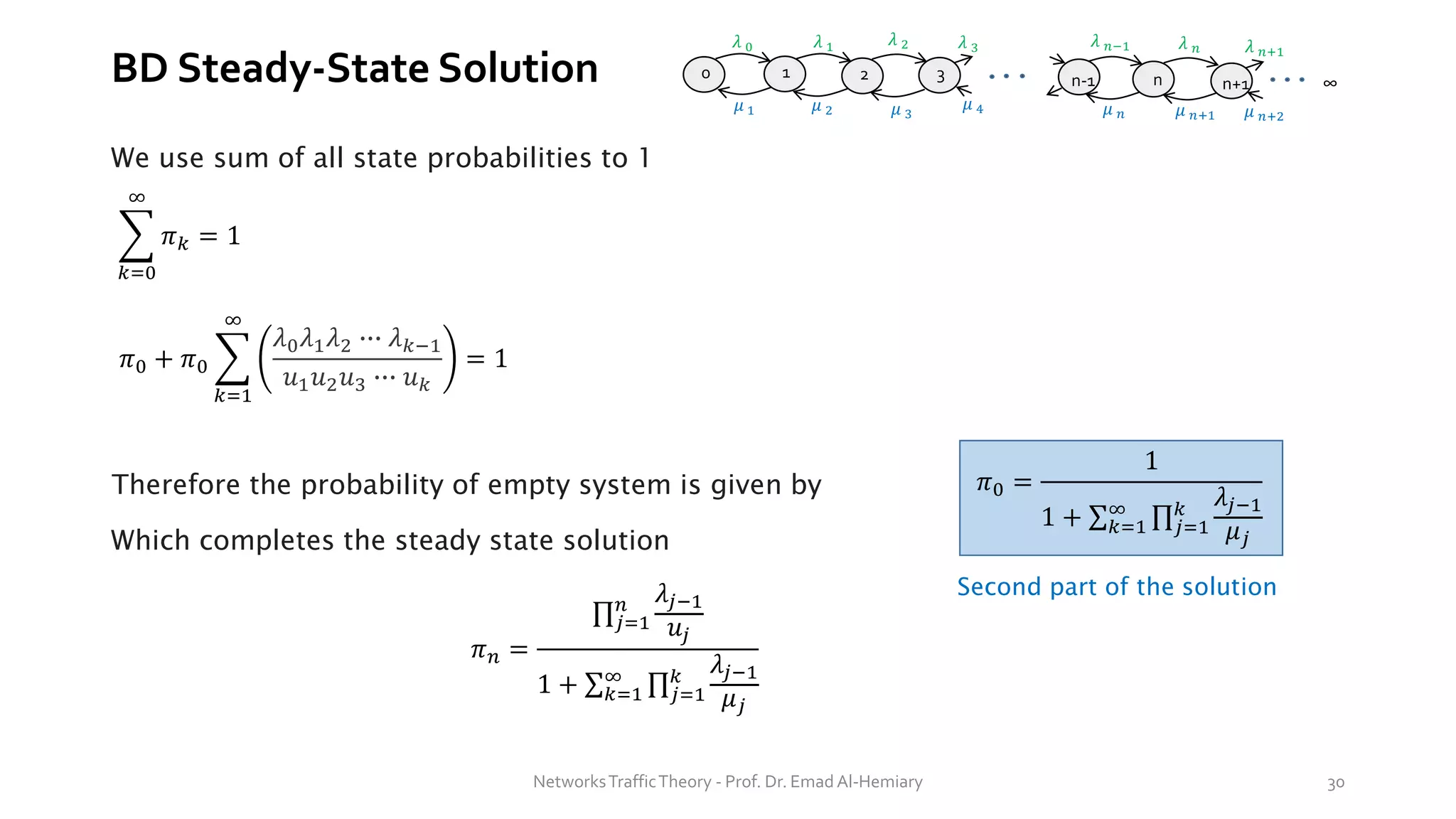
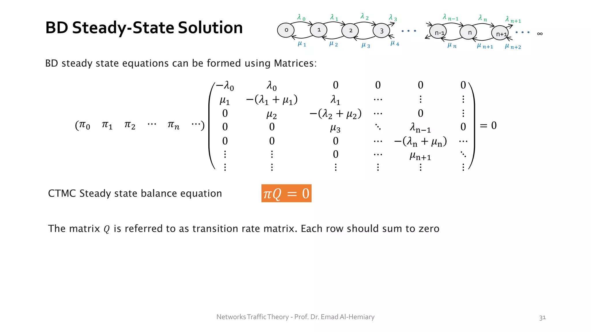
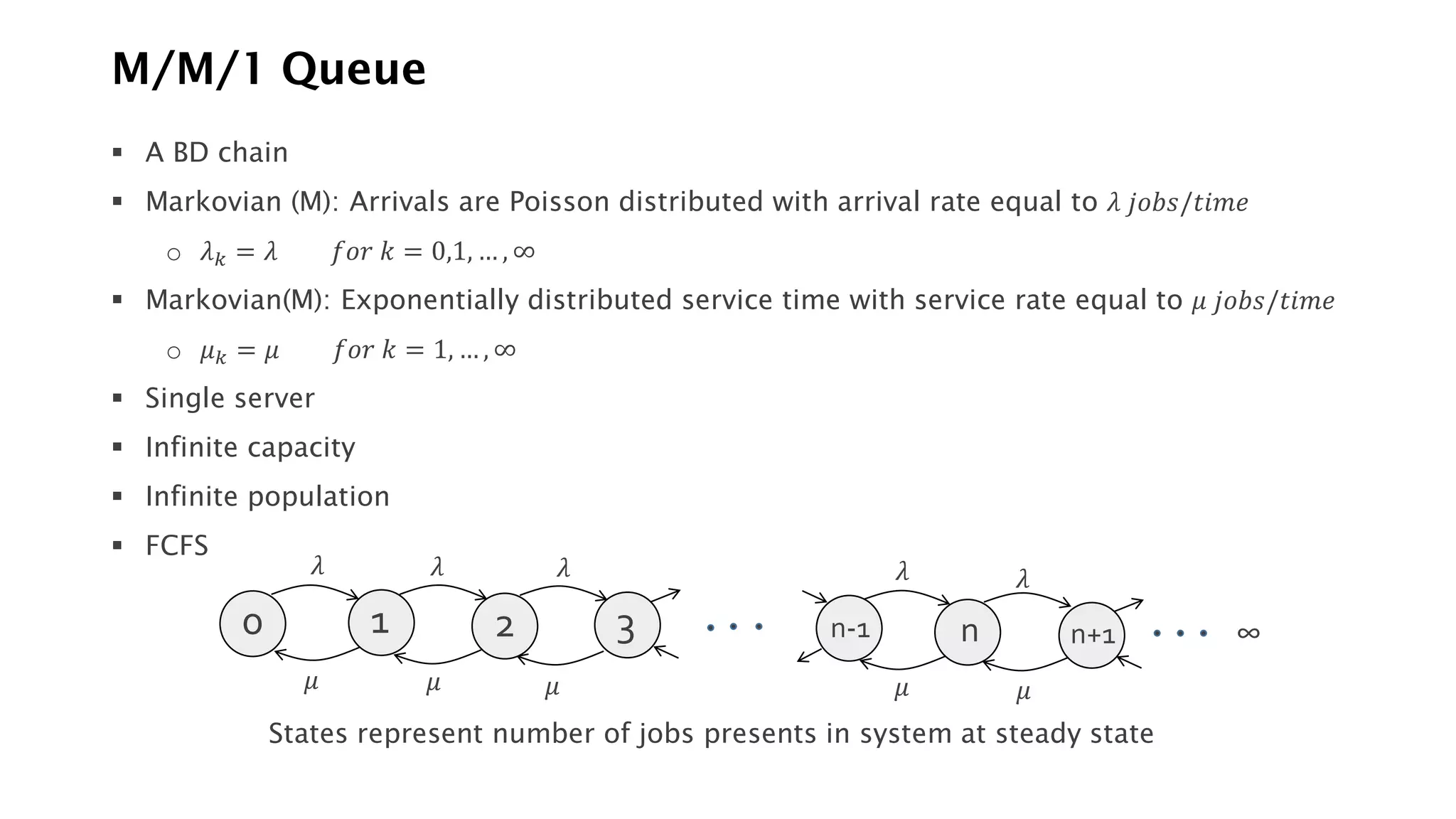
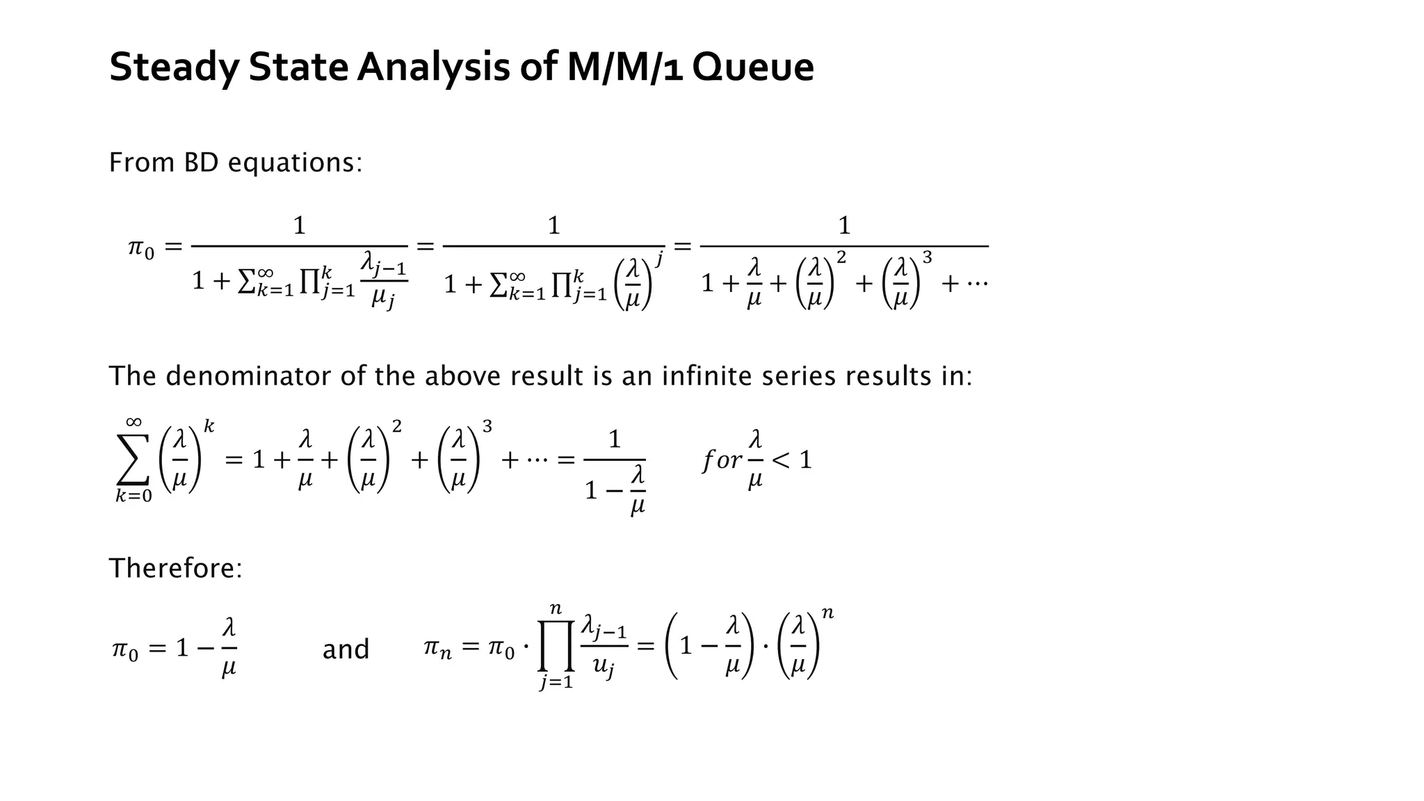
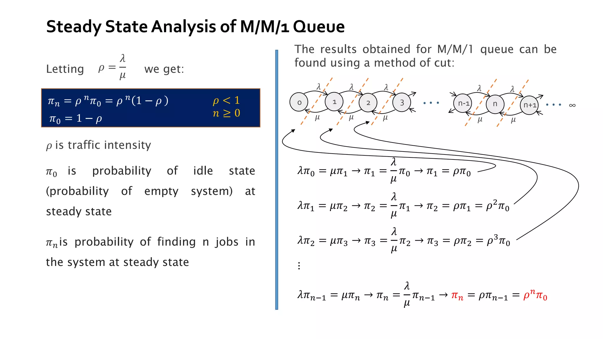
This document provides an overview of elementary queuing theory and single server queues. It defines key characteristics of queuing systems such as the arrival process, service process, number of servers, system capacity, and queue discipline. Common distributions for arrivals (Poisson) and service times (exponential) are described. Performance measures of queuing systems like delay, queue length, throughput and utilization are introduced. Other concepts covered include PASTA properties, Kendall's notation, traffic intensity, Little's Law, Markov chains, and transition probability matrices. The document serves as a lecture on introductory queuing theory concepts.

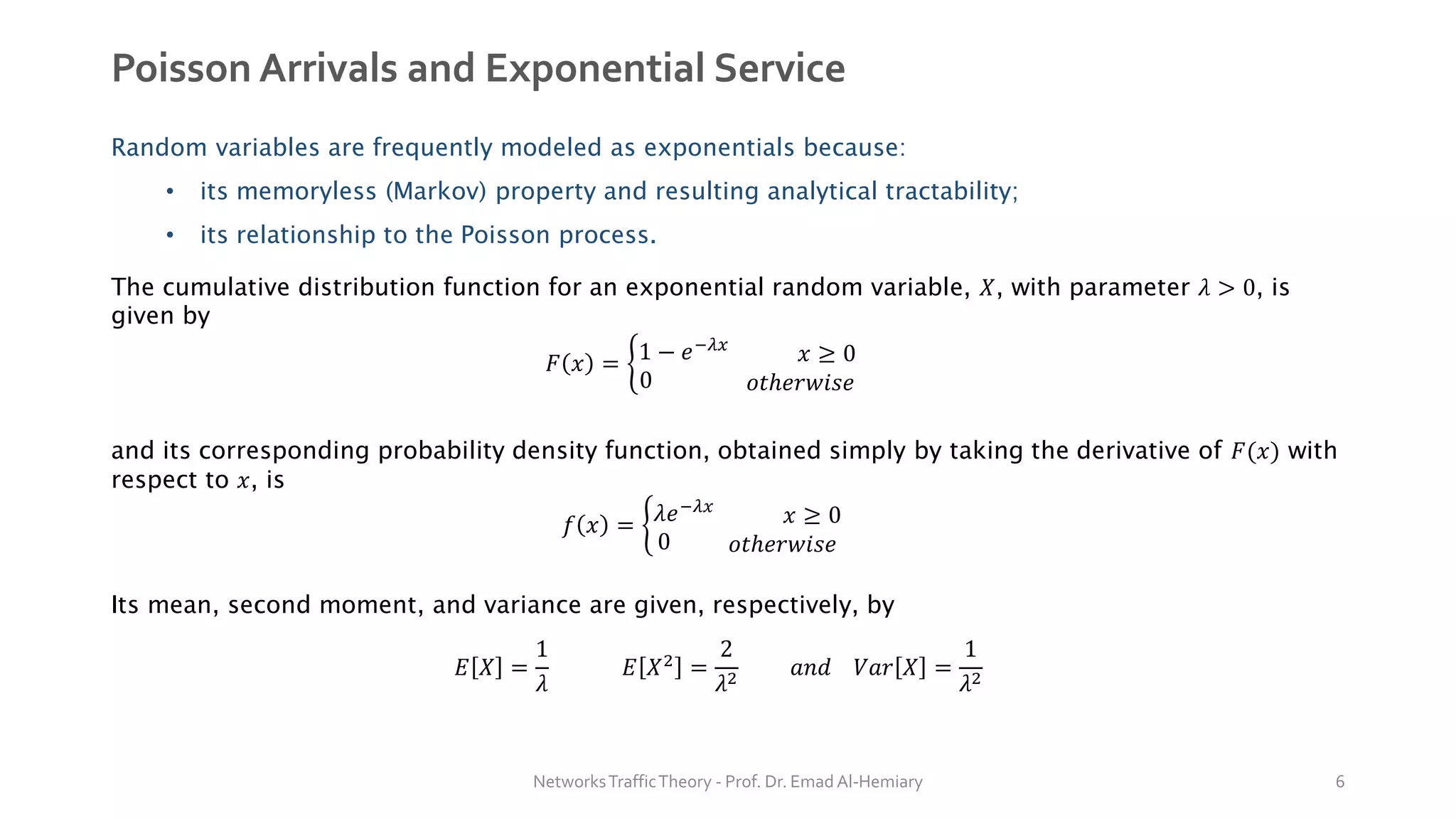
![Poisson Arrivals and Exponential Service
A Poisson process {𝑁(𝑡 ), 𝑡 ≥ 0} having rate 𝜆 ≥ 0 is a counting process with independent and stationary increments,
with 𝑁(0) = 0, and is such that the number of events that occur in any time interval of length 𝑡 has a Poisson
distribution with mean 𝜆𝑡. This means that
𝑝𝑛 𝑡 = prob 𝑁 𝑡 + 𝑠 − 𝑁 𝑠 = 𝑛 = 𝑒−𝜆𝑡
𝜆𝑡
𝑛!
𝑛 = 0,1,2, …
When n = 0, we get the probability of zero arrivals in (0,t]
𝑝0 𝑡 = 𝑒−𝜆𝑡
To compute the mean number of arrivals in an interval of length 𝑡:
𝐿 = 𝐸 𝑁 𝑡 =
𝑘=1
∞
𝑘𝑝𝑘 𝑡 =
𝑘=1
∞
𝑘𝑒−𝜆𝑡
𝜆𝑡
𝑛!
= 𝜆𝑡
𝑘=1
∞
𝜆𝑡 𝑘−1
𝑘 − 1
𝑒−𝜆𝑡
= 𝜆𝑡
𝑘=0
∞
𝜆𝑡 𝑘
𝑘!
𝑒−𝜆𝑡
= 𝜆𝑡
It is now evident why 𝜆 is referred to as the rate of the Poisson process, since the mean number of
arrivals per unit time, 𝐸[𝑁(𝑡 )]/𝑡 , is equal to 𝜆.
Finally, the mean and variance of Poisson distribution equal to 𝜆𝑡
NetworksTrafficTheory - Prof. Dr. Emad Al-Hemiary 7](https://image.slidesharecdn.com/lecture-2-01-02-2022-220327161933/75/Lecture-2-01-02-2022-pdf-7-2048.jpg)
![Mean Number in the System
In steady state, the mean number in the system is the expected value of jobs at steady state and is
given by (states represents number of jobs):
𝐿 = 𝐸[𝑁] =
𝑛=0
∞
𝑛𝑝𝑛
𝐸[∙] is the mean (expected value)
𝑛 is the state number (n = 0, 1, 2, …)
𝑝𝑛 probability of system state 𝑛
0 1 2 3 n-1 n n+1 ∞
0 jobs with
probability 𝑝0
1 jobs with
probability 𝑝1
2 jobs with
probability 𝑝2
n jobs with
probability 𝑝𝑛
n+1 jobs with
probability 𝑝𝑛+1
= 𝐿](https://image.slidesharecdn.com/lecture-2-01-02-2022-220327161933/75/Lecture-2-01-02-2022-pdf-35-2048.jpg)