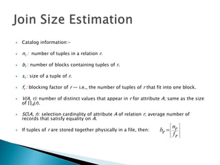
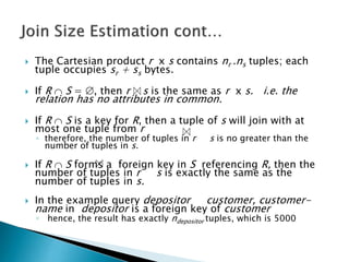
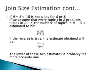
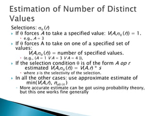
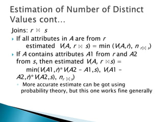
The document discusses query optimization in databases. Query optimization is the process of selecting the most efficient query evaluation plan to minimize costs and maximize performance. An optimized query will be executed faster using less system resources. Key factors considered during optimization include join size estimation, estimating the number of distinct values, and catalog information about relations.

2.  Query Optimization
 Why Query Optimization?
 Join Size Estimation?
 Estimation of Number of Distinct Values.

3.  Query optimization is the process of selecting
the most efficient query-evaluation plan from
among the many strategies usually possible
for processing a given query, especially if the
query is complex.
 In simple scenes the query optimizer come
up with query-evaluation plan that computes
the same result as a given expression, but it
is a least costly way of generating result.

4.  Faster processing of a query.
 Lesser cost per query.
 High performance of the system.
 Lesser stress on the database.
 Efficient use of database engine.
 Lesser memory is consumed.

5.  Catalog information:-
 nr : number of tuples in a relation r.
 br : number of blocks containing tuples of r.
 sr : size of a tuple of r.
 fr : blocking factor of r — i.e., the number of tuples of r that fit into one block.
 V(A, r): number of distinct values that appear in r for attribute A; same as the size
of A(r).
 SC(A, r): selection cardinality of attribute A of relation r; average number of
records that satisfy equality on A.
 If tuples of r are stored together physically in a file, then:











rf
rn
rb

6.  The Cartesian product r x s contains nr .ns tuples; each
tuple occupies sr + ss bytes.
 If R  S = , then r s is the same as r x s. i.e. the
relation has no attributes in common.
 If R  S is a key for R, then a tuple of s will join with at
most one tuple from r
◦ therefore, the number of tuples in r s is no greater than the
number of tuples in s.
 If R  S forms a foreign key in S referencing R, then the
number of tuples in r s is exactly the same as the
number of tuples in s.
 In the example query depositor customer, customer-
name in depositor is a foreign key of customer
◦ hence, the result has exactly ndepositor tuples, which is 5000

7.  If R  S = {A} is not a key for R or S.
If we assume that every tuple t in R produces
tuples in R S, the number of tuples in R S is
estimated to be:
If the reverse is true, the estimate obtained will
be:
The lower of these two estimates is probably the
more accurate one.
),( sAV
nn sr 
),( rAV
nn sr 

8. Selections:  (r)
 If  forces A to take a specified value: V(A, (r)) = 1.
 e.g., A = 3
 If  forces A to take on one of a specified set of
values:
V(A, (r)) = number of specified values.
 (e.g., (A = 1 V A = 3 V A = 4 )),
 If the selection condition  is of the form A op r
estimated V(A, (r)) = V(A.r) * s
 where s is the selectivity of the selection.
 In all the other cases: use approximate estimate of
min(V(A,r), n (r) )
◦ More accurate estimate can be got using probability theory,
but this one works fine generally

9. Joins: r s
 If all attributes in A are from r
estimated V(A, r s) = min (V(A,r), n r s)
 If A contains attributes A1 from r and A2
from s, then estimated V(A, r s) =
min(V(A1,r)*V(A2 – A1,s), V(A1 –
A2,r)*V(A2,s), nr s)
◦ More accurate estimate can be got using
probability theory, but this one works fine generally

10. THANKYOU…!!!