
Recommended
More Related Content
What's hot
What's hot (20)
Viewers also liked
Viewers also liked (20)
Similar to Signal Compression and JPEG
Similar to Signal Compression and JPEG (20)
More from guest9006ab
More from guest9006ab (14)
Recently uploaded
Recently uploaded (20)
Signal Compression and JPEG
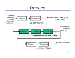
- 1. Overview Analog capturing PCM encoded or “raw” signal Sampling Fine Quantization device (“wav”, “bmp”, …) (camera, microphone) A/D CONVERTER Compressed bit stream (mp3, jpg, …) Transform Quantizer VLC encoding COMPRESSION/SOURCE CODING Channel bit stream Encipher Error protect. CHANNEL CODING -1-
- 2. Reduce the #Amplitudes 24 bit (16777200 different colors) -2-
- 3. Reduce the #Amplitudes 8 bit (256 different colors) CF 3 -3-
- 4. Reduce the #Amplitudes 6 bit (64 different colors) CF 4 -4-
- 5. Reduce the #Amplitudes 4 bit (16 different colors) CF 6 -5-
- 6. Reduce the #Amplitudes 1 bit (2 different colors) CF 24 -6-
- 7. Reduce the #Amplitudes 8 bit (256 different gray values) CF 3 -7-
- 8. Reduce the #Amplitudes 4 bit (16 different gray values) CF 6 -8-
- 9. Reduce the #Amplitudes 3 bit (8 different gray values) CF 8 -9-
- 10. Reduce the #Amplitudes 2 bit (4 different gray values) CF 12 -10-
- 11. But there are More Cleaver Ways JPEG CF 15 -11-
- 12. Why can Signals be Compressed? Because infinite accuracy of signal amplitudes is (perceptually) irrelevant 24 bit (16777200 different colors) 8 bit (256 different colors) Compression factor 3 Rate-distortion theory, scalar/vector quantization -12-
- 13. Why can Signals be Compressed? Because signal amplitudes are statistically redundant Information theory, Huffman coding -13-
- 14. Why can Signals be Compressed? Because signal amplitudes are mutually dependent 250 200 150 “S” 100 50 0 500 1000 1500 2000 2500 3000 3500 4000 4500 200 150 “O” 100 0 1000 2000 3000 4000 5000 Rate-distortion theory, transform coding -14-
- 15. Why can Signals be Compressed? Example of signal with no dependencies between successive amplitudes (Gaussian uncorrelated noise) Indeed “noise” compresses badly -15-
- 16. System Overview Analog capturing PCM encoded or “raw” signal Sampling Fine Quantization device (“wav”, “bmp”, …) (camera, microphone) A/D CONVERTER Compressed bit stream (mp3, jpg, …) Transform Quantizer VLC encoding COMPRESSION/SOURCE CODING Channel bit stream Encipher Error protect. CHANNEL CODING -16-
- 17. Quantization Even Uniform Odd Uniform Q(x) p(x) Even Non-uniform Odd Non-uniform Quantizer level more probable -17-
- 18. Information and Entropy More Probable Less information -18-
- 19. Huffman Code y4 0.51 0.51 (0) 0 y3 0.20 0.29 (0) 0.49 (1) 11 y2 0.14 0.15 (0) 0.20 (1) 101 y5 0.08 0.08 (0) 0.14 (1) 1000 y6 0.04 0.04 (0) 0.07 (1) 10010 y1 0.02 0.02 (0) 0.03 (1) 100110 y7 0.005 (0) 0.01 (1) 1001110 y0 0.005 (1) 1001111 -19-
- 20. Run Length Coding Representing “0 0 0 0 0 0 0 0 1 1 0 0 0 0 0 0 1 1 1 1 1 0 0 ...” “Runs” : 8 (“zeros”) 2 (“ones”) 6 (“zeros”) 5 (“ones”) …… The run lengths are also encoded (e.g. with Huffman coding) Efficient transforms (like DCT) used in compression produce A lot of “zero” values And a “few” (significant) non-zero values Typical symbol sequences to be coded “5 1 0 0 0 0 0 0 0 3 0 0 6 0 0 0 0 1 0 0 0 0 …..” will be done by {zero-run, non-zero symbol/0} pairs Here: “{0,5},{0,1},{7,3},{2,6},{4,1},…..” The pairs will now be assigned a Huffman code This is used in JPEG -20-
- 21. General Compression System Analog capturing PCM encoded or “raw” signal Sampling Fine Quantization device (“wav”, “bmp”, …) (camera, microphone) A/D CONVERTER Compressed bit stream (mp3, jpg, …) Transform Quantizer VLC encoding COMPRESSION/SOURCE CODING Channel bit stream Encipher Error protect. CHANNEL CODING -21-
- 22. Correlation in Signals - I Meaningful signals are often highly predictable: Δx(n)=x(n)-x(n-1) 100 4 250 200 150 0 100 50 100 0 500 1000 1500 2000 2500 3000 3500 4000 4500 500 1000 1500 2000 2500 3000 3500 4000 4500 (Linear) Predictability has something to do with the autocorrelation function n -22-
- 23. Principle of Differential PCM x(n) Δx(n) Δx*(n) 001010010 - Q VLC ˆ x ( n) Previous Predict x(n) signal values (“past”) x(n-1), x(n-2), x(n-3), …. -23-
- 24. Works Really Good - I Variance = 3240 -24-
- 25. Works Really Good - II Variance = 315 -25-
- 26. DPCM Signal to be encoded Prediction difference/error Predicted signal Reconstructed signal -26-
- 27. What Linear Predictor to Use? Examples: PCM x( n ) = 0 $ Simple differences x ( n ) = ~ ( n − 1) $ x Average last two samples x( n ) = h1 ~ ( n − 1) + h2 ~ ( n − 2) $ x x N x( n) = ∑ hk ~( n − k ) General linear predictor $ x k =1 -27-
- 28. DPCM on Images Same principle as 1-D Definition of “Past” and “Future” in Images: Predictions: horizontal (scan line) vertical (column) 2-dimensional -28-
- 29. General Compression System Analog capturing PCM encoded or “raw” signal Sampling Fine Quantization device (“wav”, “bmp”, …) (camera, microphone) A/D CONVERTER Compressed bit stream (mp3, jpg, …) Transform Quantizer VLC encoding COMPRESSION/SOURCE CODING Channel bit stream Encipher Error protect. CHANNEL CODING -29-
- 30. Transform Coding channel x(n) x T θ θ$ T-1 $ x $ x(n) Decorrelating Correlating Inverse Vectorize Transform Q Q-1 Transform Vectorize Which transform used? -30-
- 31. Removing Correlation - I 100 50 0 50 100 0 200 400 600 800 1000 40 x2 ⎛ x1 ⎞ ⎜ ⎟ ⎝ x2 ⎠ 20 x1 40 20 0 20 40 20 -31- 40
- 32. Removing Correlation - II 100 50 0 50 100 0 200 400 600 800 1000 40 x2 θ1 ⎛ x1 ⎞ σ22 Rotate the ⎜ ⎟ coordinates ⎝ x2 ⎠ 20 σ12 x1 40 20 0 20 40 θ2 20 -32- 40
- 33. Removing Correlation - III 50 0 50 0 100 200 300 400 500 600 700 800 900 40 x2 θ1 ⎛ x1 ⎞ ⎜ ⎟ 20 ⎝ x2 ⎠ x1 40 20 0 20 40 θ2 20 -33- 40
- 34. Decomposition N ⎛θ1 ⎞ ⎛ t11 L t1,N ⎞⎛ x1 ⎞ ⎜ ⎟ ⎜ , ⎟⎜ ⎟ θk = ∑t n =1 k ,n xn k = 1, 2 , K , N θ = ⎜ M ⎟ = ⎜ M O M ⎟⎜ M ⎟ = Tx N ⎜ ⎟ ⎜ ⎠ ⎜ ⎟ ⎝θN⎠ ⎝tN,1 L tN,N⎟⎝ xN⎠ xn = ∑θ k =1 k t n ,k n = 1, 2 , K , N N x = ∑θ k =1 k t k = θ1 t 1 + θ 2 t 2 + L + θ N t N t1 0.707 0.25 -0.125 x 0.0 0.0 -0.702 3.165 1.718 2.266 4.516 1.020 0.638 3.377 0.063 -0.2 (Example) t8 -0.025 θ -34-
- 35. Discrete Cosine Transform N=8 t1 0.354 0.49 0.462 0.416 0.354 0.278 0.191 0.098 t2 0.354 0.416 0.191 0.098 0.354 0.49 0.462 0.278 0.354 0.278 0.191 0.49 0.354 0.098 0.462 0.416 t3 0.354 0.098 0.462 0.278 0.354 0.416 0.191 0.49 T = t 0.354 0.098 0.462 0.278 0.354 0.416 0.191 0.49 t4 0.354 0.278 0.191 0.49 0.354 0.098 0.462 0.416 t5 0.354 0.416 0.191 0.098 0.354 0.49 0.462 0.278 0.354 0.49 0.462 0.416 0.354 0.278 0.191 0.098 t6 (All picture compression standards t7 implement this matrix in a clever way) t8 -35-
- 36. Image Transforms - I 6 0 1 1 1 -1 1 1 1 -1 = 4 1 -1 2 4 6 1 1 1 -1 -1 -1 -1 1 x m,n t11 t12 t21 t22 θ11 θ12 θ21 θ22 -36-
- 37. Basis Images for 2-D DCT -37-
- 38. Discrete Cosine Transform (DCT) (1) 8 rows 8 pixels -38-
- 39. Discrete Cosine Transform (DCT) (2) 64 pixels Cosine patterns/DCT basis functions -39-
- 40. Discrete Cosine Transform (DCT) (3) 89 8 8 1 0 -1 1 0 2 3 0 0 0 0 0 0 0 1 0 1 0 0 0 0 0 0 0 1 0 0 0 0 2 0 0 1 0 1 0 0 64 pixels 0 0 -1 1 0 0 0 0 0 0 0 1 0 0 0 0 0 0 0 0 0 0 0 0 Cosine patterns/DCT basis functions -40-
- 41. Discrete Cosine Transform (DCT) (4) ! -41-
- 42. 2-D DCT of Picture - I -42-
- 43. 2-D DCT of Image - II Low freq uencies A DCT coefficients is a weight of particular DCT basis function. High fre quencies -43-
- 44. “Grouped” DCT Coefficients -44-
- 45. JPEG Compression System -45-
- 46. DCT Weight Matrix and Quantization Quantization: ⎛ θk ,l ⎞ θ$k ,l = Q[θk ,l ] = round⎜ ' ⎜Q N ⎟ ⎟ ⎝ k ,l ⎠ Recommended JPEG normalization matrix ⎡ 16 11 10 16 24 40 51 61 ⎤ ⎢ 12 12 14 19 26 58 60 55 ⎥ ⎢ ⎥ ⎢ 14 13 16 24 40 57 69 56 ⎥ ⎢ ⎥ N k ,l = ⎢ 14 17 22 29 51 87 80 62 ⎥ ⎢ 18 22 37 56 68 109 103 77 ⎥ ⎢ ⎥ ⎢ 24 35 55 64 81 104 113 92 ⎥ ⎢ 49 64 78 87 103 121 120 101⎥ ⎢ ⎥ ⎢ 72 ⎣ 92 95 98 112 100 103 99 ⎥⎦ -46-
- 47. User Controllable Quality User has control over a “quality parameter” that runs from 100 (“perfect”) to 0 (“extremely poor”) Q' Parameter used to scale the normalization matrix 6 5 4 3 2 1 0 Q 0 10 20 30 40 50 60 70 80 90 100 Increasing quality -47-
- 48. Entropy coding Runlength coding Huffman coded then huffman or arithmetic coding -48-
- 49. Example ⎡139 144 149 153 155 155 155 155⎤ ⎢ ⎥ ⎢144 151 153 156 159 156 156 156 ⎥ ⎢ ⎥ ⎢150 155 160 163 158 156 156 156 ⎥ ⎢ ⎥ ⎢159 161 162 160 160 159 159 159 ⎥ f = ⎢ ⎥ k, l ⎢159 160 161 162 162 155 155 155 ⎥ ⎢ ⎥ ⎢161 161 161 161 160 157 157 157 ⎥ ⎢ ⎥ ⎢ ⎢162 162 161 163 162 157 157 157 ⎥ ⎥ ⎢ ⎣162 162 161 161 163 158 158 158 ⎥ ⎦ DCT transform is exactly defined in average * 8 ⎡1260 −1 − 12 −5 2 −2 3 1 ⎤ ⎢ ⎥ JPEG standard ⎢ − 23 − 17 −6 −3 −3 0 0 − 1⎥ ⎢ ⎥ ⎢ − 11 −9 −2 2 0 −1 −1 0⎥ ⎢ ⎥ ⎢ −7 −2 0 1 1 0 0 0⎥ θ =⎢ ⎢ −1 ⎥ k, l ⎢ −1 1 2 0 −1 1 1⎥ ⎥ ⎢ 2 0 2 0 −1 1 1 − 1⎥ ⎢ ⎥ ⎢ ⎢ −1 0 0 −1 0 2 1 − 1⎥ ⎥ ⎢ ⎣ −3 2 −4 −2 2 1 −1 0⎥⎦ -49-
- 50. Example ⎡ 79 0 −1 0 0 0 0 0⎤ ⎢ ⎥ ⎢− 2 −1 0 0 0 0 0 0⎥ ⎢ ⎥ ⎢−1 −1 0 0 0 0 0 0⎥ ⎢ ⎥ ⎢ 0 0 0 0 0 0 0 0⎥ θ$ = ⎢ ⎥ k,l ⎢ 0 0 0 0 0 0 0 0⎥ Quantization ⎢ ⎥ ⎢ 0 using Q’ = 1 ⎢ 0 0 0 0 0 0 0⎥ ⎥ ⎢ ⎢ 0 0 0 0 0 0 0 0⎥ ⎥ ⎢ ⎣ 0 0 0 0 0 0 0 0⎥ ⎦ DC: Difference with quantized DC coefficient of previous block is Huffman encoded AC: Zig-zag scan coefficients, and convert to (zero run- length, amplitude) combinations: (79) 0 -2 -1 -1 -1 0 0 -1 EOB {1,-2}{0,-1}{0,-1}{0,-1} {2,-1} EOB -50-
- 51. VLC Coding of AC Coefficients The (zero run-length, amplitudes) are put into categories Category AC Coefficient Range 1 -1,1 2 -3,-2,2,3 3 -7,...,-4,4,...,7 4 -15,...,-8,8,...,15 5 -31,...,-16,16,...,31 6 -63,...,-32,32,...,63 7 -127,...,-64,64,...,127 8 -255,...,-128,128,...,255 9 -511,...,-256,256,...,511 10 -1023,...,-512,512,...,1023 The (zero run-length, categories) are Huffman encoded The sign and offset into a category are FLC encoded (required #bits = category number) -51-
- 52. JPEG AC Huffman Table Z ero R u n C a teg o ry C o d e len g th C o d ewo rd 0 1 2 00 0 2 2 01 0 3 3 100 0 4 4 1011 0 5 5 11010 0 6 6 111000 0 7 7 1111000 . . . . . . . 1 1 4 1100 1 2 6 111001 1 3 7 1111001 1 4 9 111110110 . . . . . . . . 2 1 5 11011 2 2 8 11111000 . . . . . . . . 3 1 6 111010 3 2 9 111110111 . . . . . . . . 4 1 6 111011 5 1 7 1111010 6 1 7 1111011 7 1 8 11111001 8 1 8 11111010 9 1 9 111111000 10 1 9 111111001 11 1 9 111111010 . . . . . . . . EOB 4 1010 -52-
- 53. Example - III The series {1,-2}{0,-1}{0,-1}{0,-1} {2,-1} EOB now becomes 111001 01/00 0/00 0/00 0/11011 0/1010 Bit rate for AC coefficients in this DCT block 27 bits/64 pixels = 0.42 bit/pixel -53-
- 54. Ordering of Coefficient -54-
- 55. Sequential Encoding -55-
- 56. Acknowledgement Prof. Inald Lagendijk, Delft University of Technology Also try the software VcDemo http://ict.ewi.tudelft.nl/index.php?Itemid=124 -56-