![MBA-H2040 Quantitative Techniques for Managers
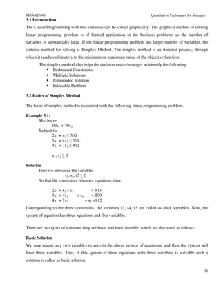
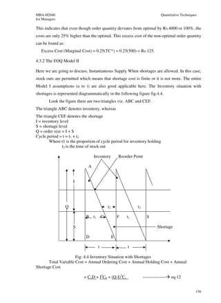
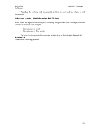
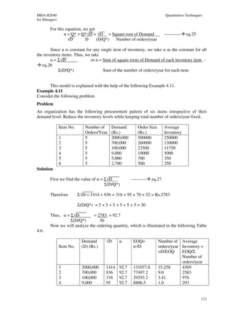
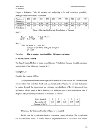
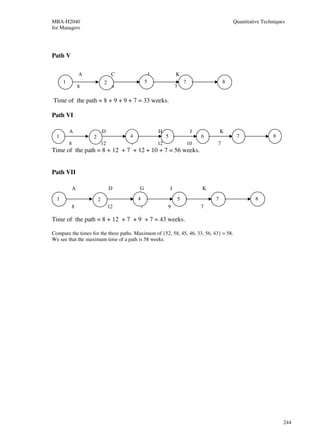
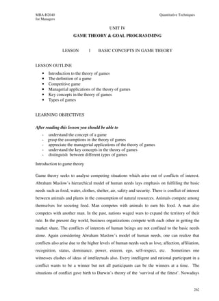
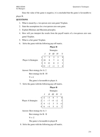
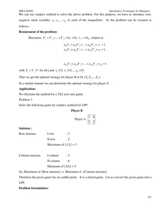
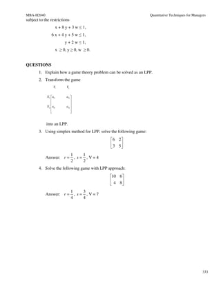
(military) OPERATIONS] was coined as a suitable description of this new branch of applied science.
The first team was selected from amongst the scientists of the radar research group the same day.
1939
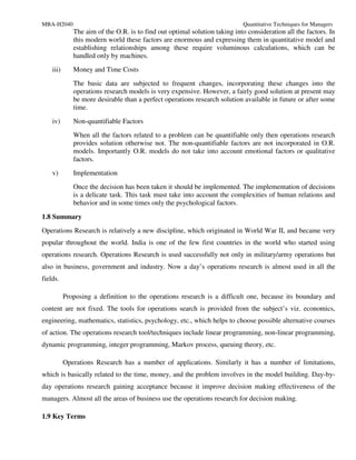
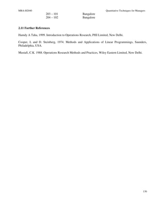
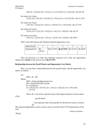
In the summer of 1939 Britain held what was to be its last pre-war air defence exercise. It involved some
33,000 men, 1,300 aircraft, 110 antiaircraft guns, 700 searchlights, and 100 barrage balloons. This
exercise showed a great improvement in the operation of the air defence warning and control system.
The contribution made by the OR team was so apparent that the Air Officer Commander-in-Chief RAF
Fighter Command (Air Chief Marshal Sir Hugh Dowding) requested that, on the outbreak of war, they
should be attached to his headquarters at Stanmore in north London.
Initially, they were designated the "Stanmore Research Section". In 1941 they were redesignated
the "Operational Research Section" when the term was formalised and officially accepted, and similar
sections set up at other RAF commands.
1940
On May 15th 1940, with German forces advancing rapidly in France, Stanmore Research Section was
asked to analyses a French request for ten additional fighter squadrons (12 aircraft a squadron - so 120
aircraft in all) when losses were running at some three squadrons every two days (i.e. 36 aircraft every 2
days). They prepared graphs for Winston Churchill (the British Prime Minister of the time), based upon
a study of current daily losses and replacement rates, indicating how rapidly such a move would deplete
fighter strength. No aircraft were sent and most of those currently in France were recalled.
This is held by some to be the most strategic contribution to the course of the war made by OR
(as the aircraft and pilots saved were consequently available for the successful air defense of Britain, the
Battle of Britain).
1941 onward
In 1941, an Operational Research Section (ORS) was established in Coastal Command which was to
carry out some of the most well-known OR work in World War II.
The responsibility of Coastal Command was, to a large extent, the flying of long-range sorties by
single aircraft with the object of sighting and attacking surfaced U-boats (German submarines). The
technology of the time meant that (unlike modern day submarines) surfacing was necessary to recharge
batteries, vent the boat of fumes and recharge air tanks. Moreover U-boats were much faster on the
surface than underwater as well as being less easily detected by sonar.](https://image.slidesharecdn.com/qtformanagers-101217142149-phpapp02/85/Qualitative-Technique-for-managers-5-320.jpg)

![MBA-H2040 Quantitative Techniques for Managers
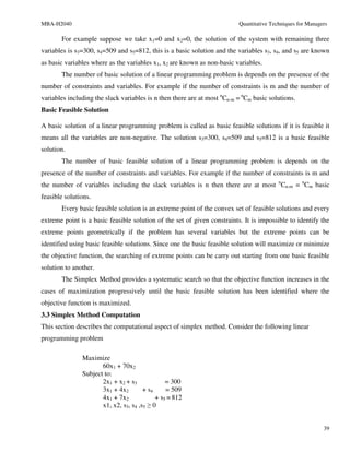
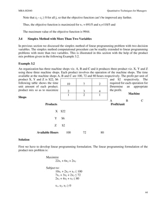
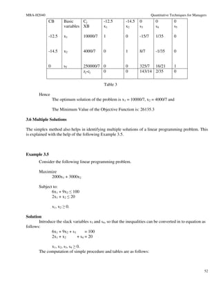
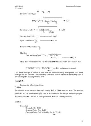
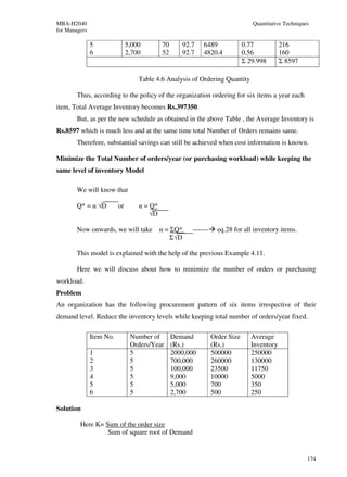
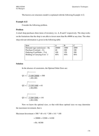
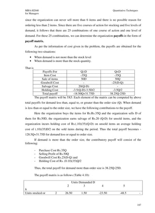
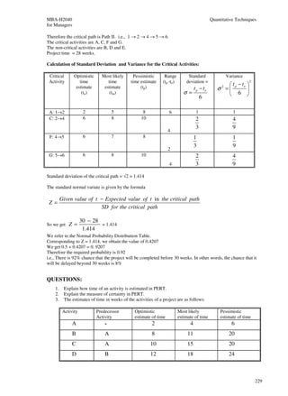
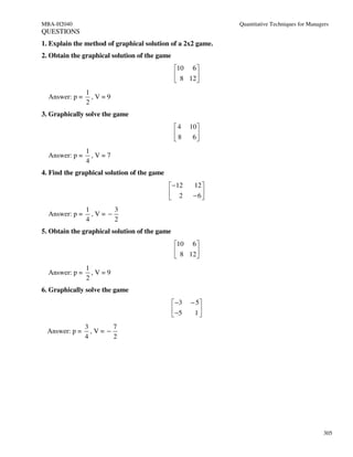
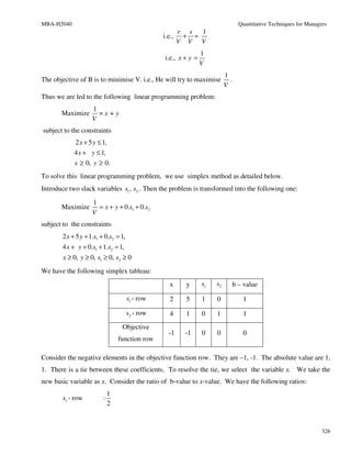
2. Let xj be the incoming basic variable and the corresponding elements of the jth row column be
denoted by Y1j, Y2j and Y3j respectively. If the present values of the basic variables are XB1,
XB2 and XB3 respectively, then we can compute.
Min [XB1/Y1j, XB2/Y2j, XB3/Y3j] for Y1j, Y2j, Y3j>0.
Note that if any Yij≤0, this need not be included in the comparison. If the minimum occurs
corresponding to XBr/Yrj then the rth basic variable will become non-basic in the next iteration.
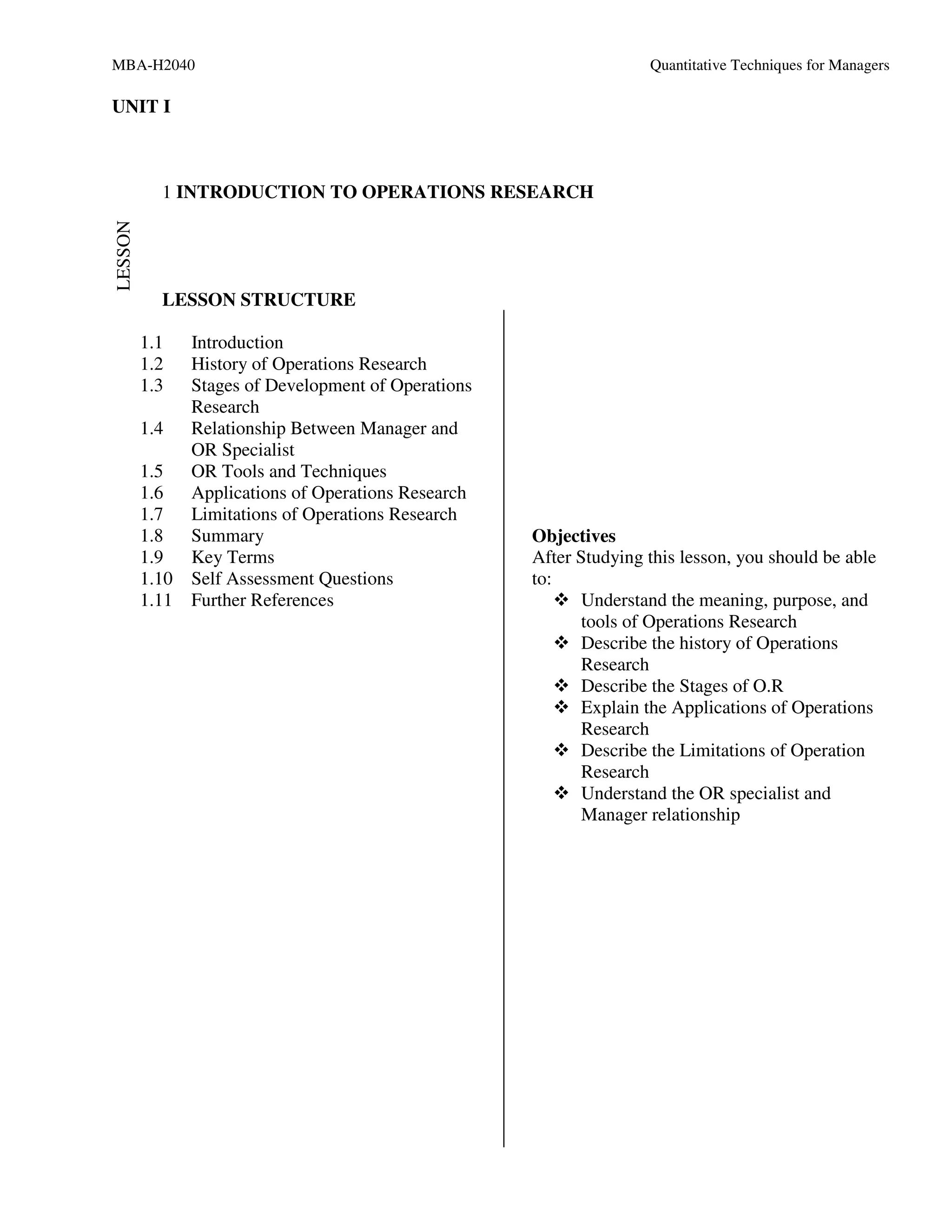
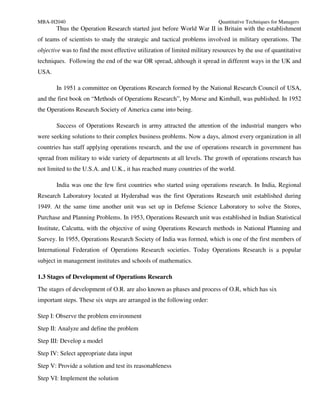
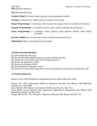
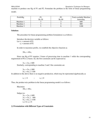
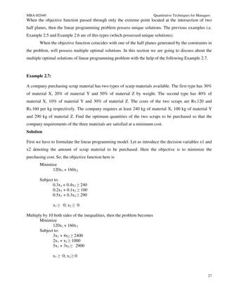
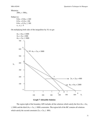
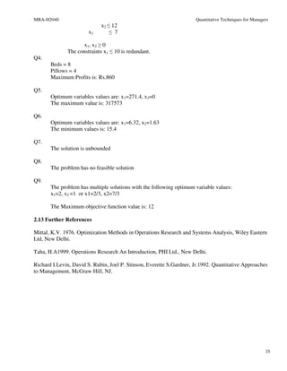
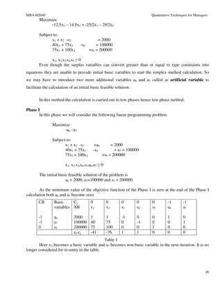
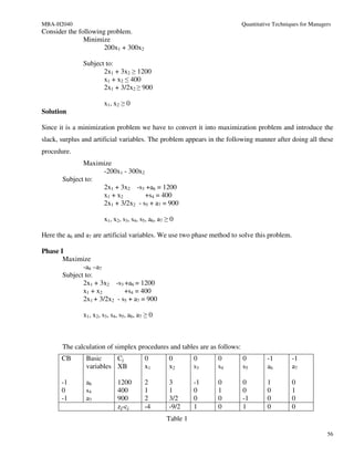
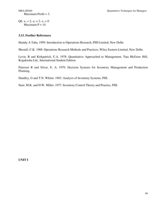
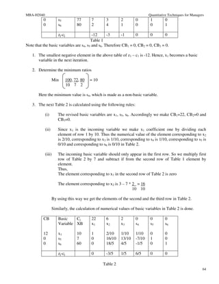
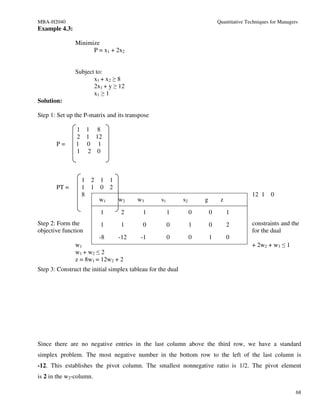
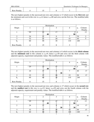
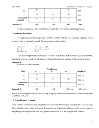
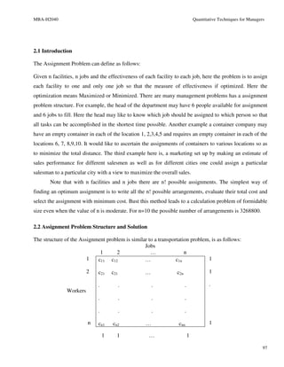
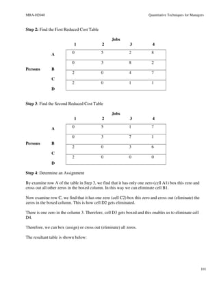
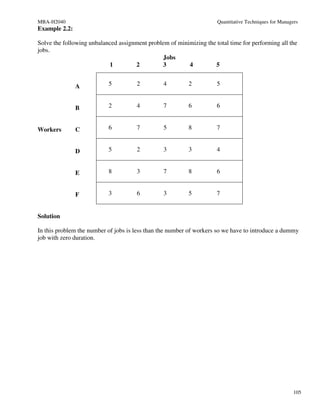
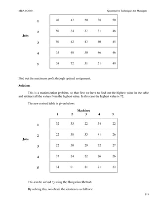
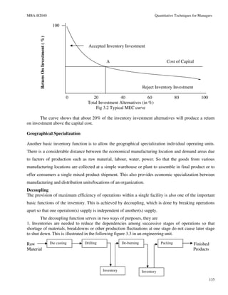
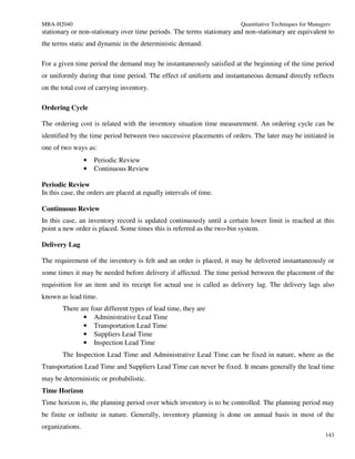
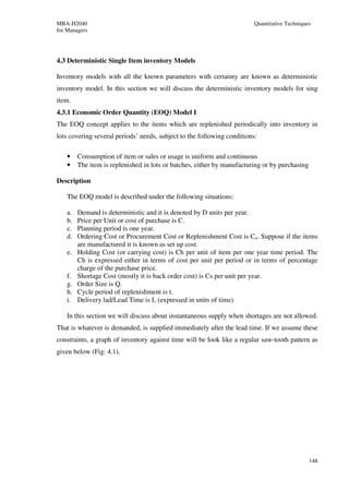
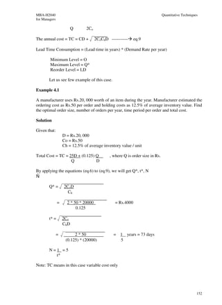
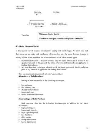
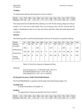
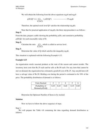
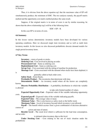
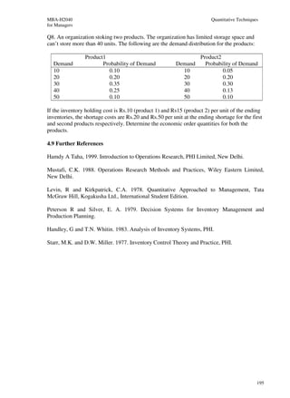
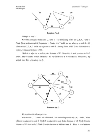
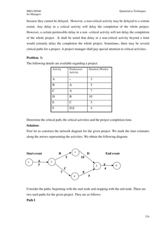
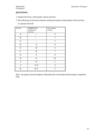
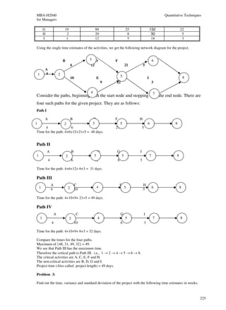
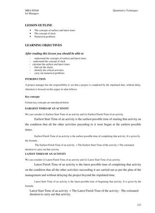
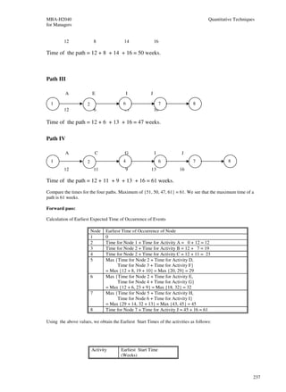
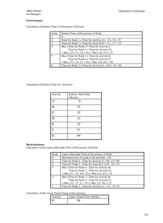
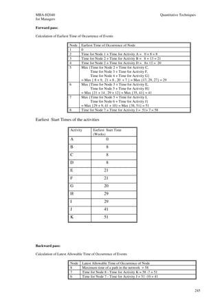
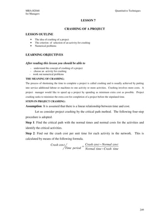
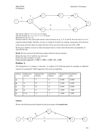
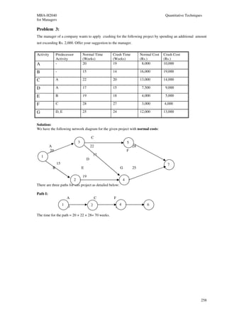
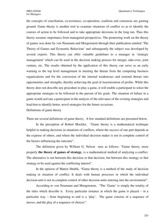
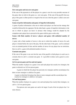
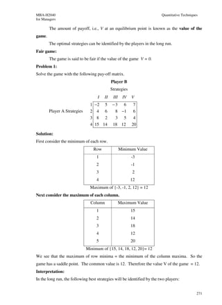
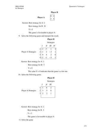
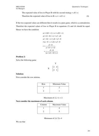
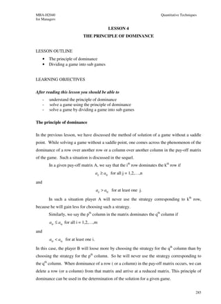
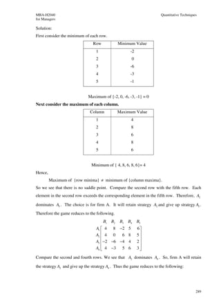
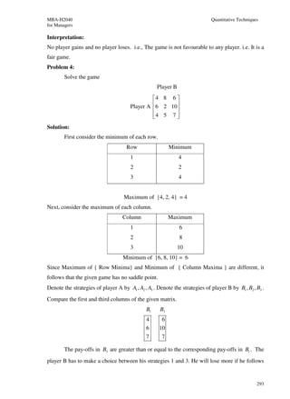
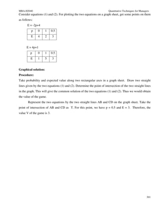
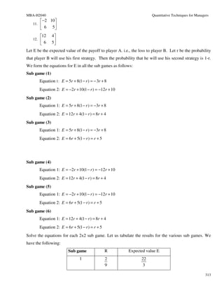
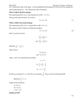
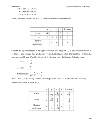
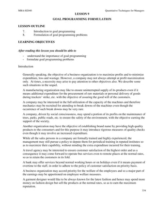
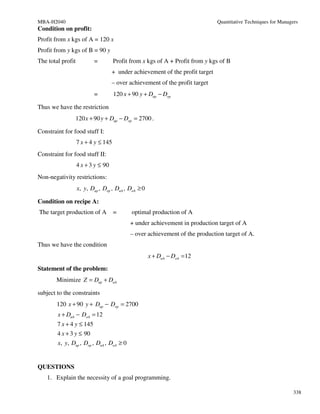
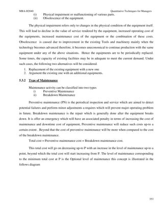
3. Using the following rules the Table 2 is computed from the Table 1.
i. The revised basic variables are s3, s4 and x2. Accordingly, we make CB1=0, CB2=0
and CB3=70.
ii. As x2 is the incoming basic variable we make the coefficient of x2 one by dividing
each element of row-3 by 7. Thus the numerical value of the element corresponding
to x1 is 4/7, corresponding to s5 is 1/7 in Table 2.
iii. The incoming basic variable should appear only in the third row. So we multiply the
third-row of Table 2 by 1 and subtract it from the first-row of Table 1 element by
element. Thus the element corresponding to x2 in the first-row of Table 2 is 0.
Therefore the element corresponding to x1 is
2-1*4/7=10/7 and the element corresponding to s5 is
0-1*1/7=-1/7
In this way we obtain the elements of the first and the second row in Table 2. In Table 2 the
numerical values can also be calculated in a similar way.
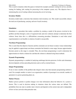
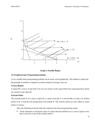
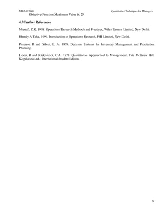
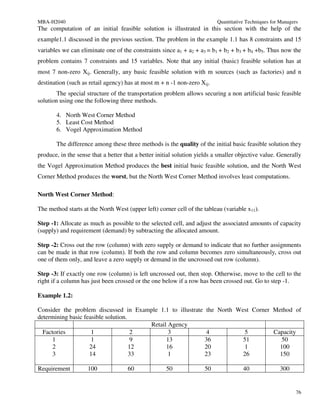
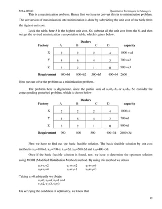
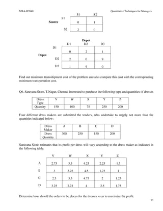
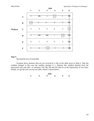
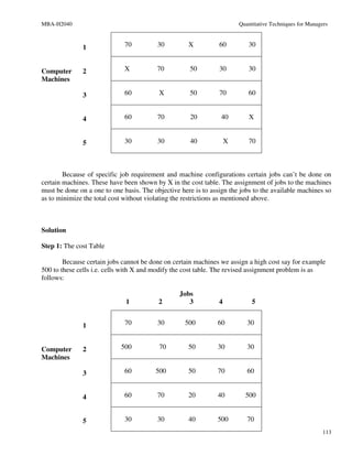
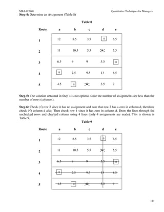
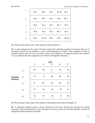
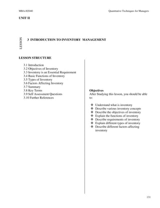
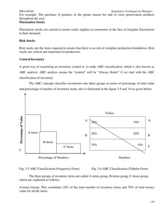
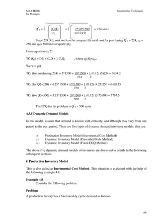
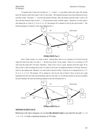
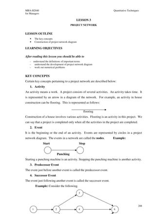
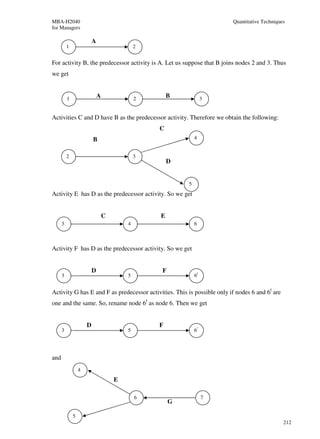
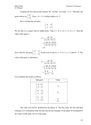
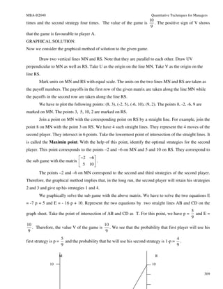
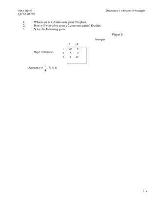
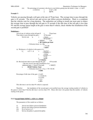
CB Basic Cj 60 70 0 0 0
Variables XB x1 x2 s3 s4 s5
0 s3 184 10/7 0 1 0 -1/7
0 s4 45 5/7 0 0 1 -4/7
70 x2 116 4/7 1 0 0 1/7
zj-cj -140/7 0 0 0 70/7
Table 2
Let CB1, CB2, Cb3 be the coefficients of the basic variables in the objective function. For
example in Table 2 CB1=0, CB2=0 and CB3=70. Suppose corresponding to a variable J, the quantity zj is
defined as zj=CB1, Y1+CB2, Y2j+CB3Y3j. Then the z-row can also be represented as Zj-Cj.
For example:
z1 - c1 = 10/7*0+5/7*0+70*4/7-60 = -140/7
z5 – c5 = -1/7*0-4/7*0+1/7*70-0 = 70/7
1. Now we apply rule (1) to Table 2. Here the only negative zj-cj is z1-c1 = -140/7
Hence x1 should become a basic variable at the next iteration.
42](https://image.slidesharecdn.com/qtformanagers-101217142149-phpapp02/85/Qualitative-Technique-for-managers-42-320.jpg)


![MBA-H2040 Quantitative Techniques
for Managers
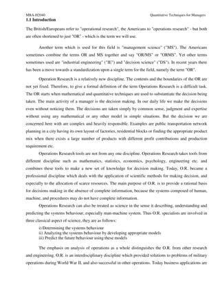
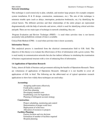
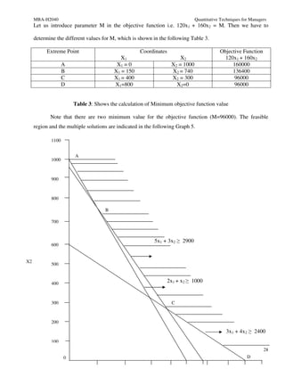
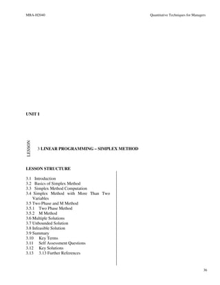
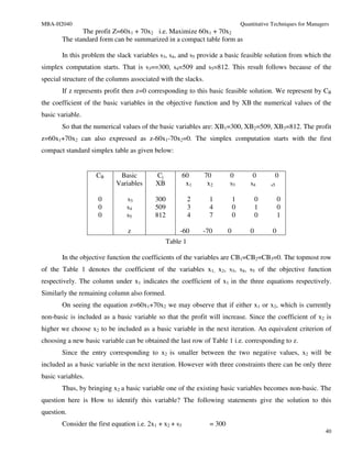
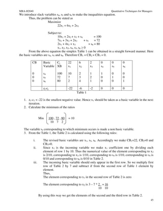
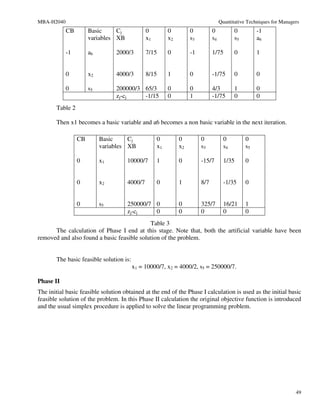
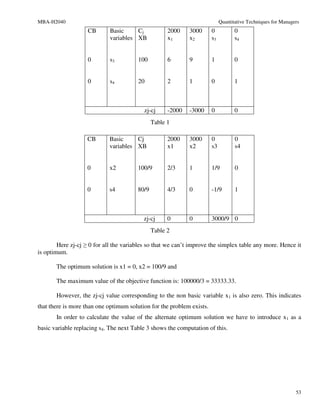
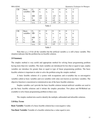
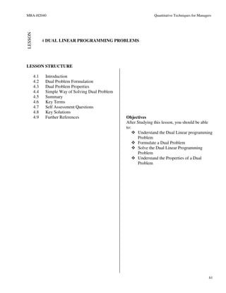
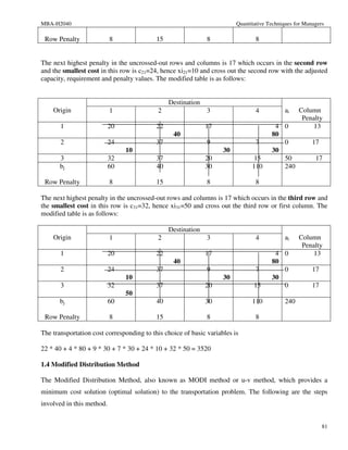
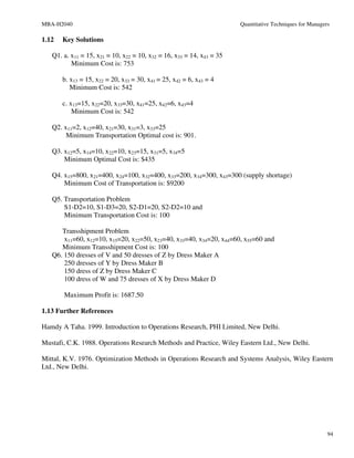
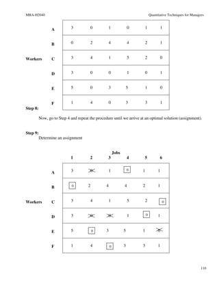
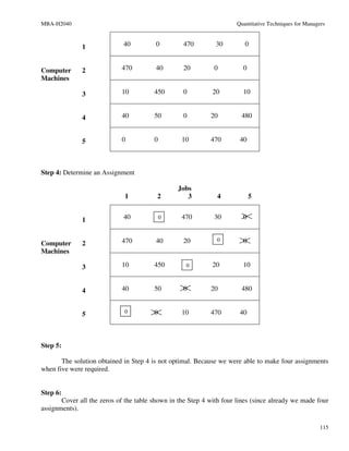
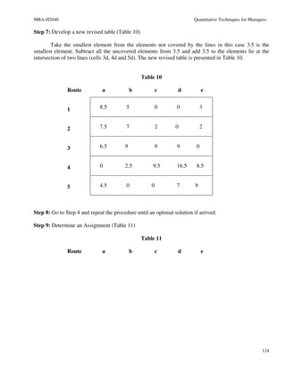
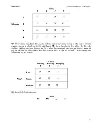
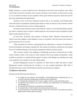
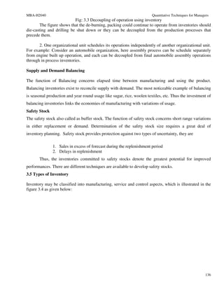
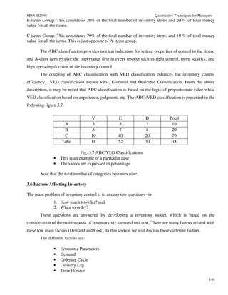
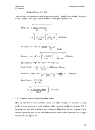
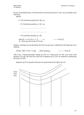
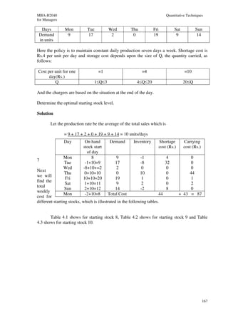
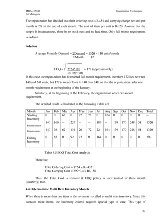
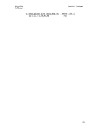
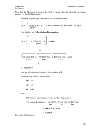
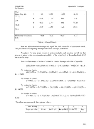
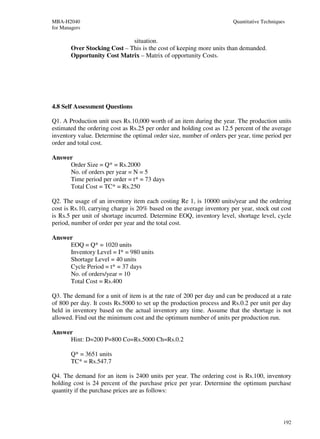
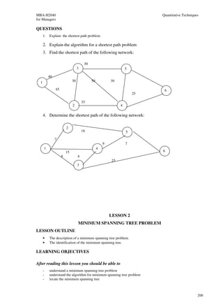
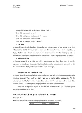
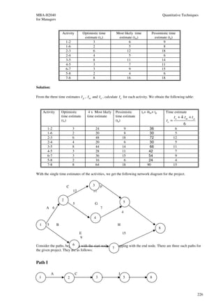
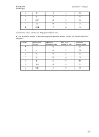
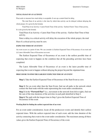
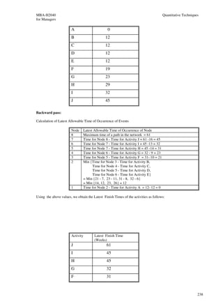
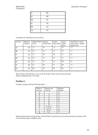
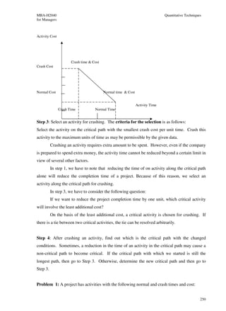
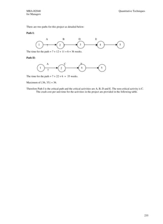
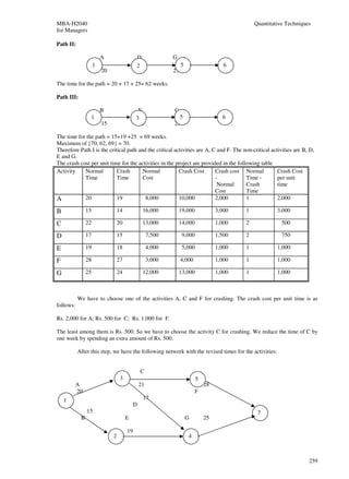
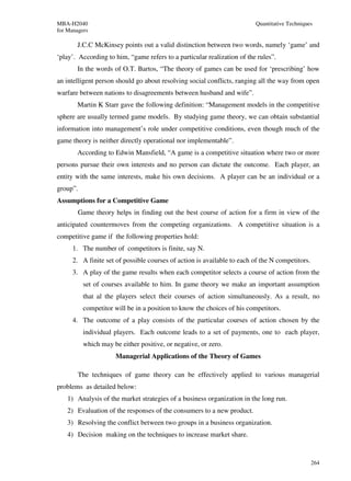
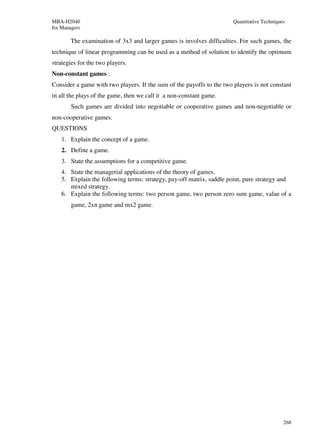
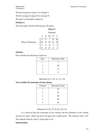
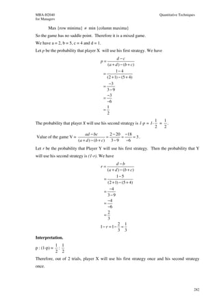
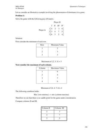
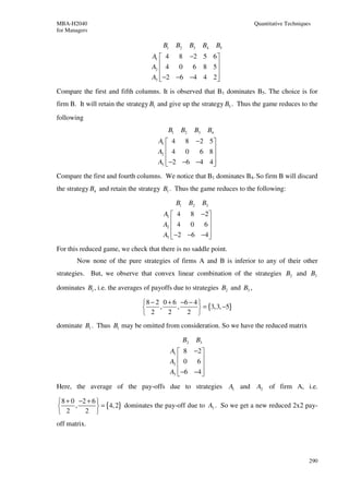
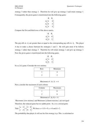
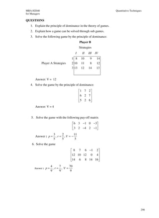
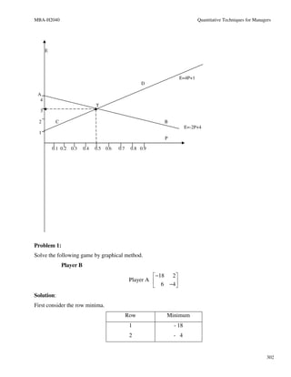
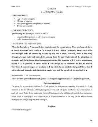
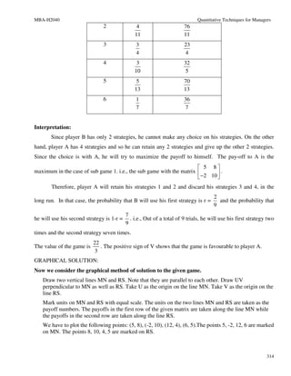
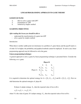
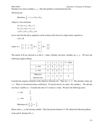
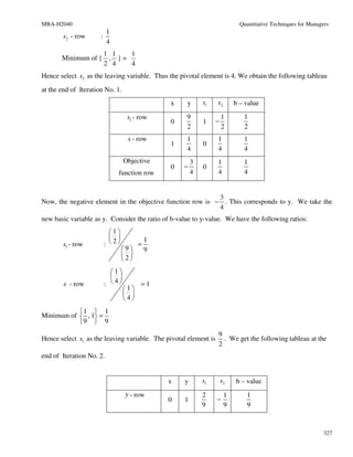
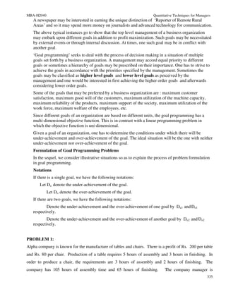
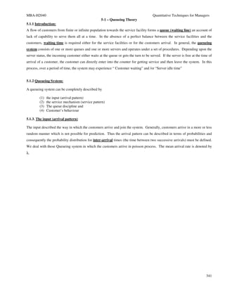
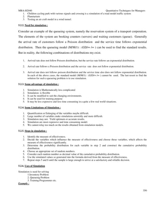
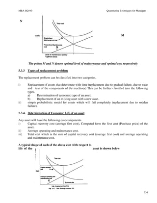
ap + c(1 − p) = bp + d (1 − p)
ap − bp = (1 − p)[d − c]
p ( a − b) = (d − c ) − p (d − c )
p ( a − b) + p ( d − c ) = d −c
p (a − b + d − c) = d −c
d −c
p =
(a + d ) − (b + c)
a + d −b−c−d +c
1− p =
(a + d ) − (b + c)
a−b
=
(a + d ) − (b + c)
The number of times A The number of times A d −c a−b
{ }:{ }= :
will use first strategy will use second strategy (a + d ) − (b + c) (a + d ) − (b + c)
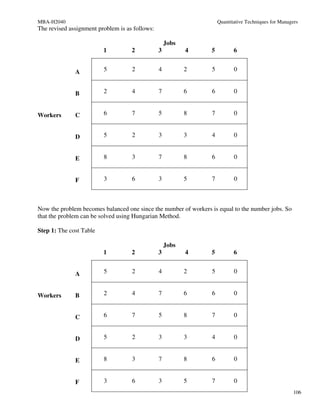
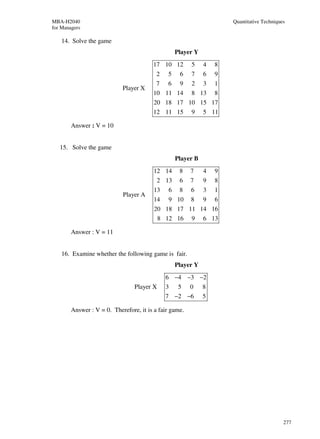
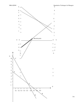
The expected pay-off to Player A
= ap + c(1 − p )
= c + p (a − c )
(d − c)(a − c)
=c+
(a + d ) − (b + c)
c {(a + d ) − (b + c)} + (d − c)(a − c)
=
(a + d ) − (b + c)
ac + cd − bc − c 2 + ad − cd − ac + c 2 )
=
(a + d ) − (b + c)
ad − bc
=
(a + d ) − (b + c)
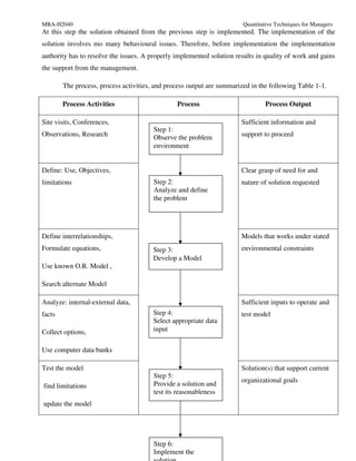
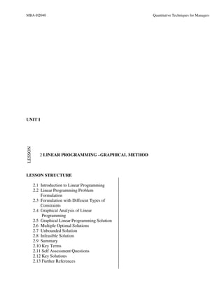
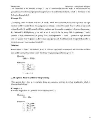
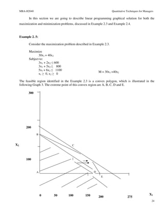
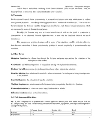
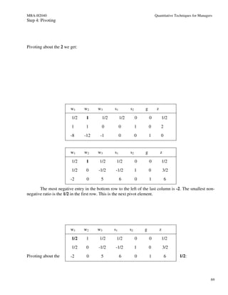
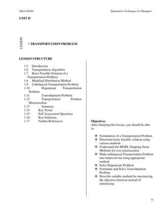
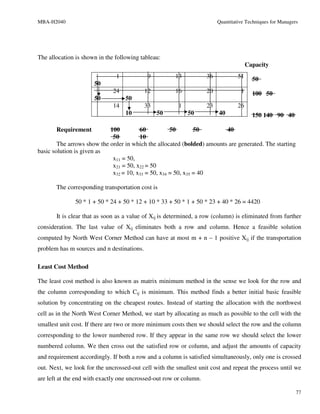
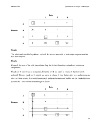
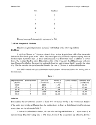
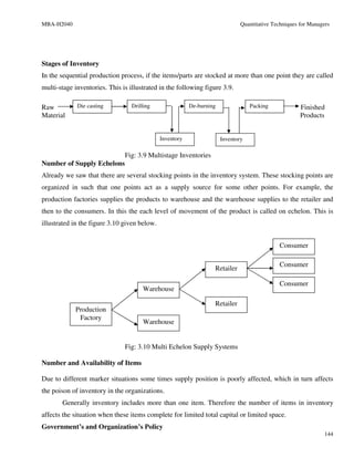
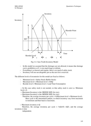
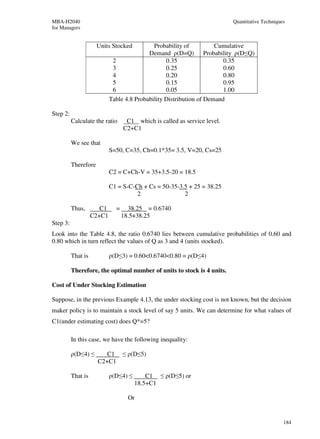
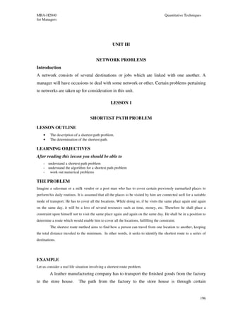
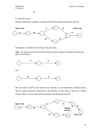
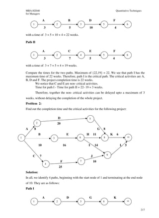
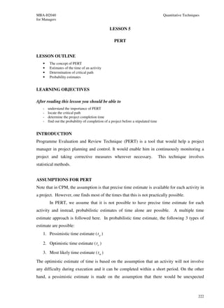
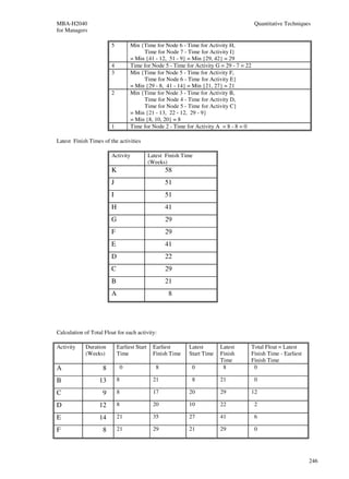
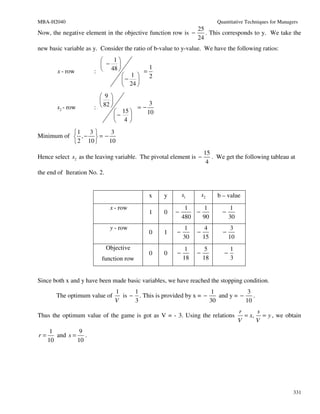
Therefore, the value V of the game is
ad − bc
(a + d ) − (b + c)
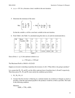
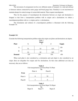
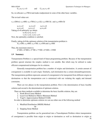
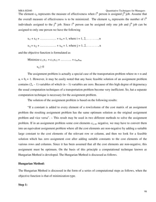
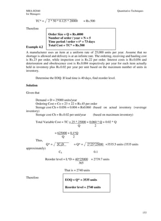
To find the number of times that B will use his first strategy and second strategy:
Let the probability that B will use his first strategy be r. Then the probability that B will use
his second strategy is 1-r.
When A use his first strategy
The expected value of loss to Player B with his first strategy = ar
The expected value of loss to Player B with his second strategy = b(1-r)
Therefore the expected value of loss to B = ar + b(1-r) (3)
When A use his second strategy
The expected value of loss to Player B with his first strategy = cr
280](https://image.slidesharecdn.com/qtformanagers-101217142149-phpapp02/85/Qualitative-Technique-for-managers-280-320.jpg)


![MBA-H2040 Quantitative Techniques for Managers
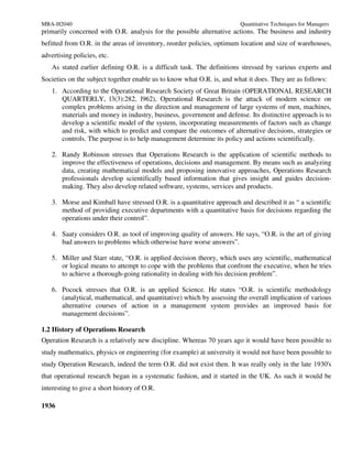
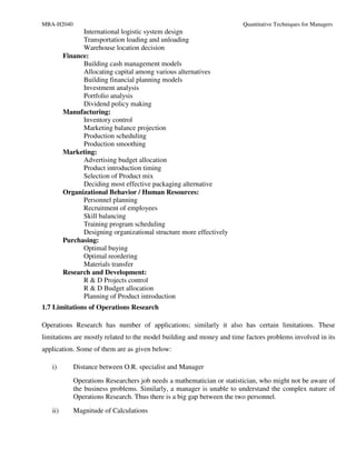
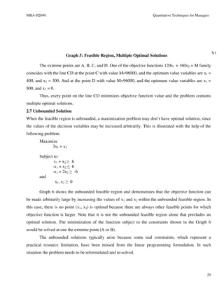
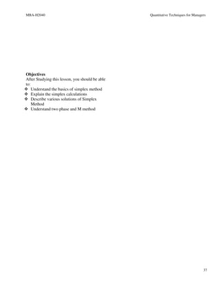
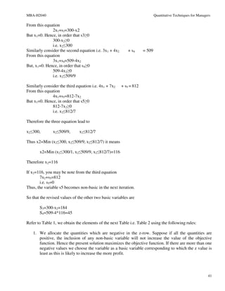
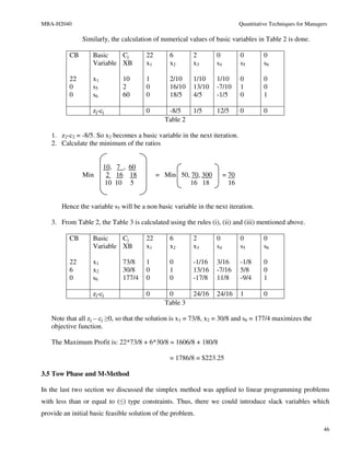
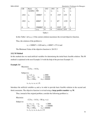
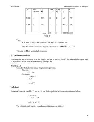
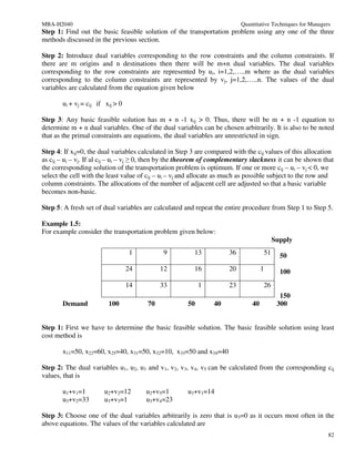
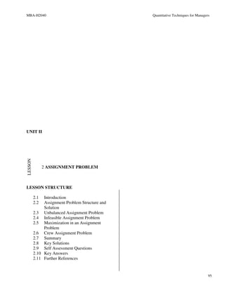
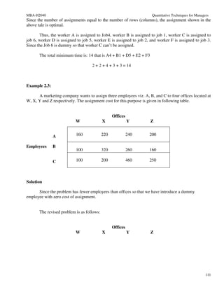
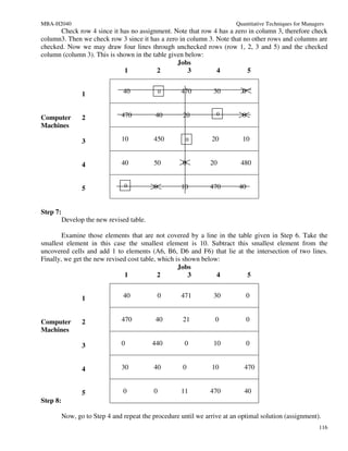
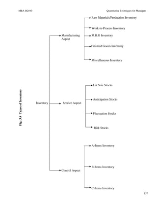
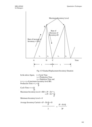
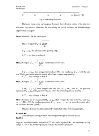
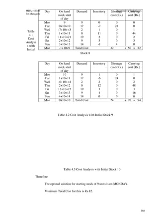
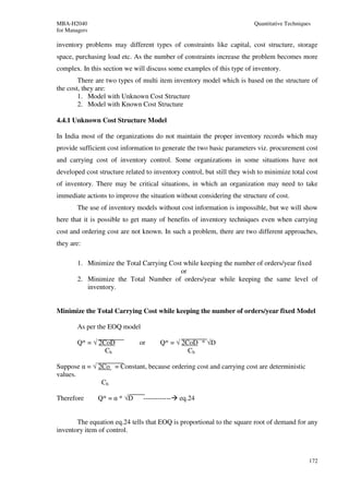
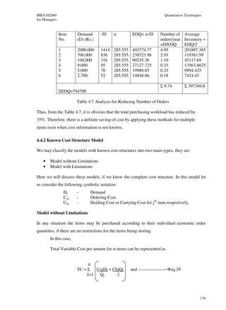
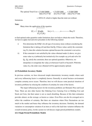
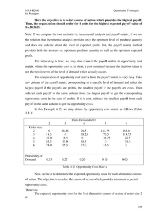
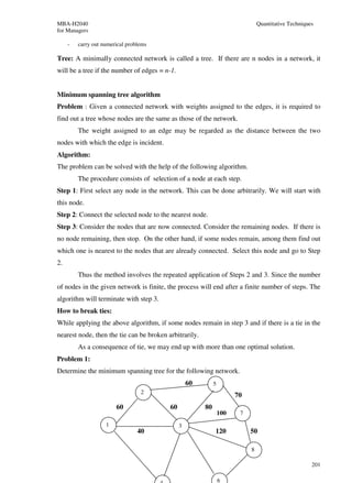
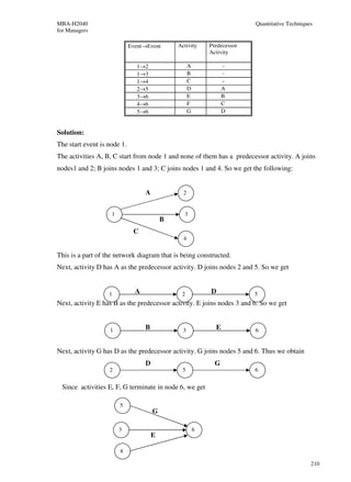
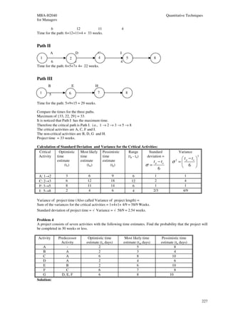
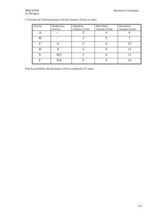
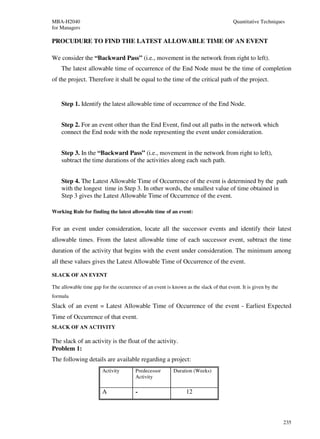
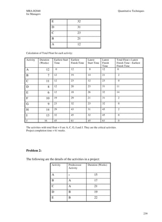
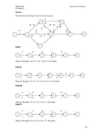
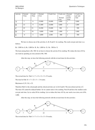
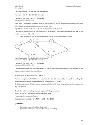
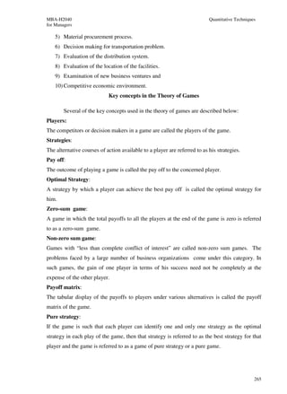
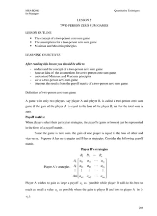
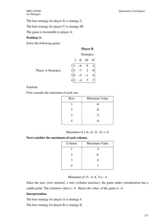
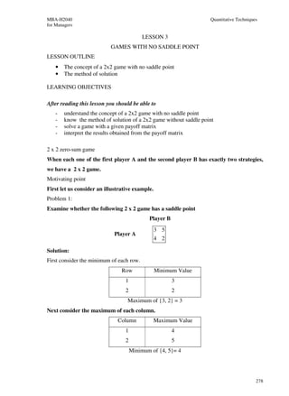
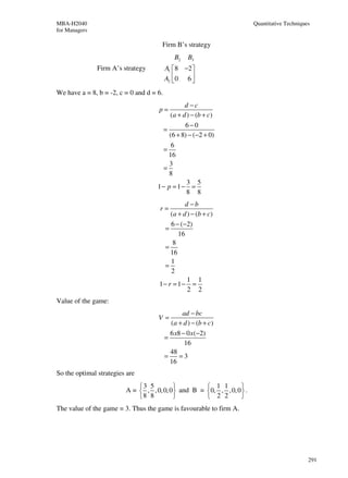
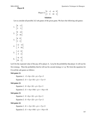
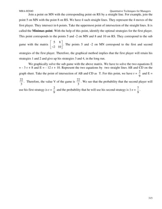
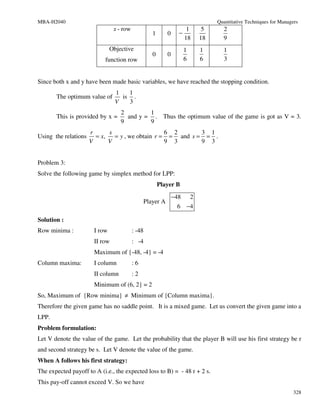
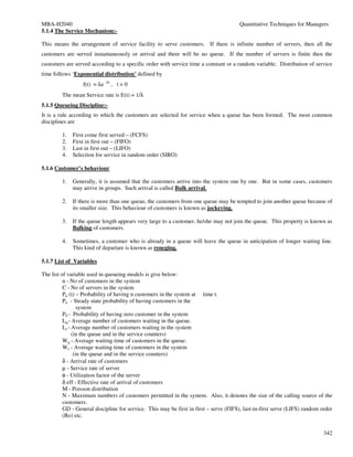
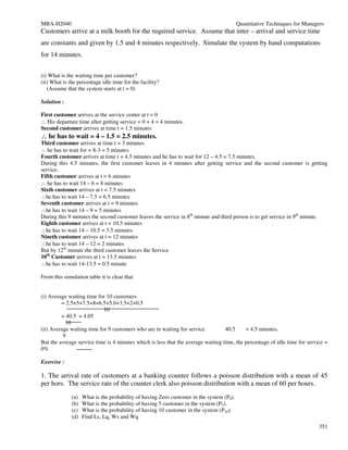
= φ - (1 - φ) φ
1-φ
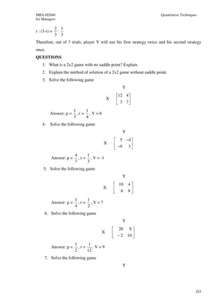
Lq = φ2
of φ
Average waiting time 1 - customers in the system
(in the queue and in the service station) = Ws
= Ws = Ls = φ
δ (1 - φ)δ
=φ x 1 = 1
1-φ µφ µ(1 - φ)
(Since δ = µφ )
= 1
µ - µφ
= 1
µ-δ
Ws = 1
µ-δ
Wq = Average waiting time of customers in the
queue.
= Lq / δ = [1 / δ] [ φ2 / [1- φ]]
= 1 / µφ [ φ2 / [1- φ]]
= φ Since µφ = δ
µ - µφ
Wq = φ
µ-δ
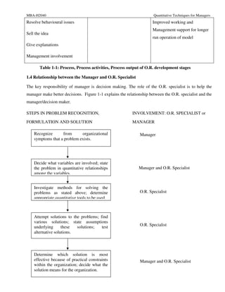
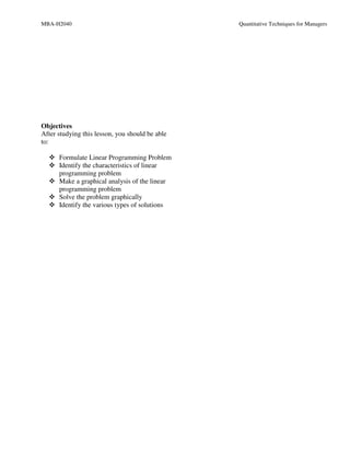
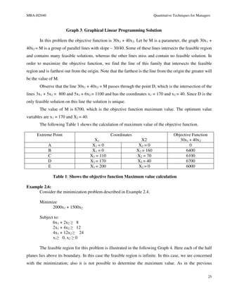
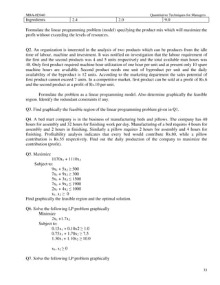
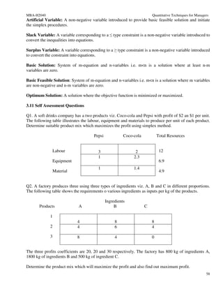
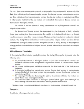
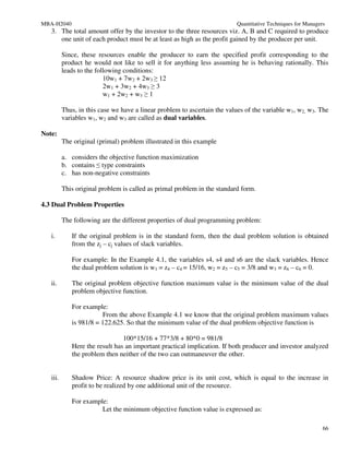
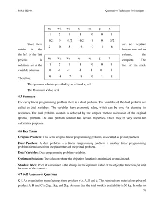
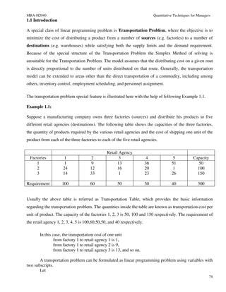
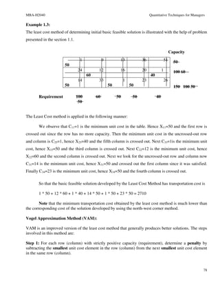
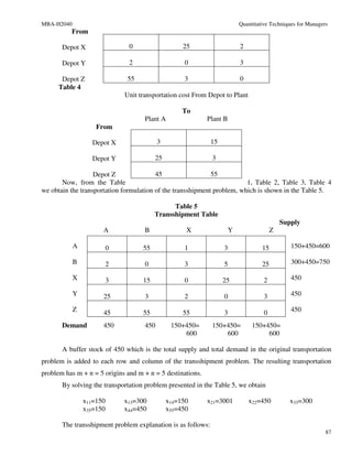
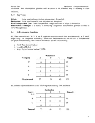
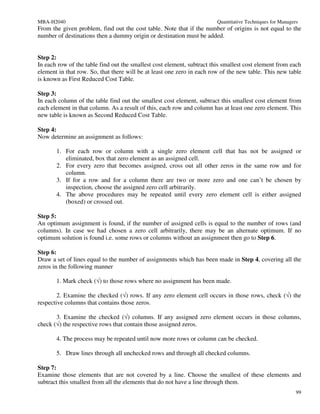
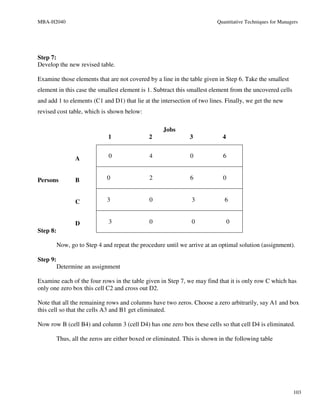
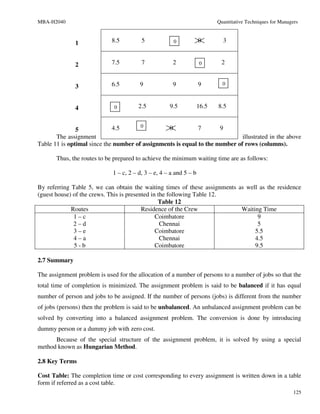
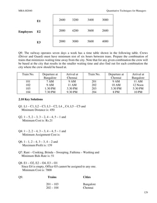
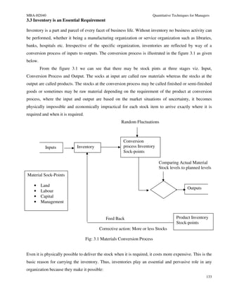
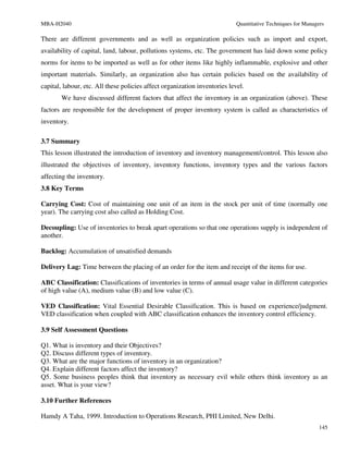
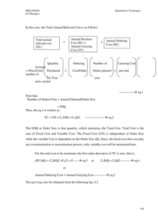
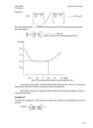
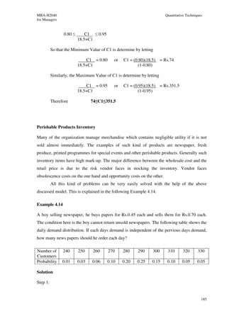
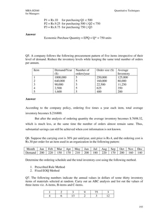
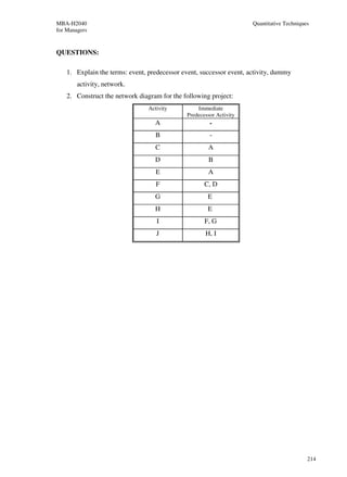
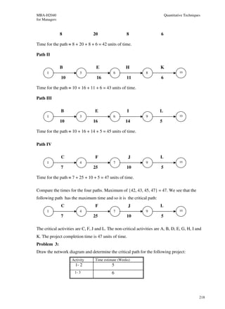
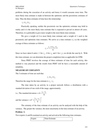
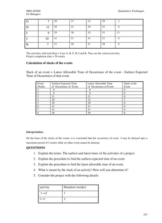
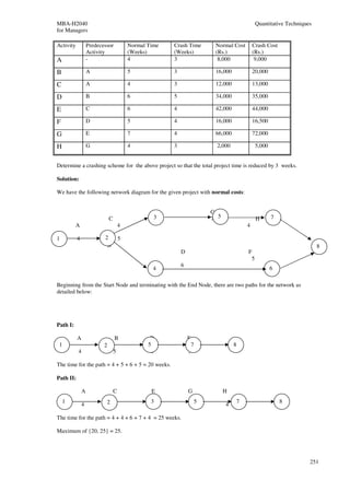
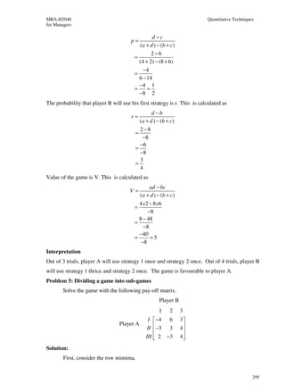
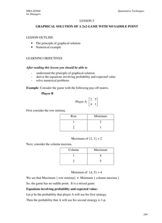
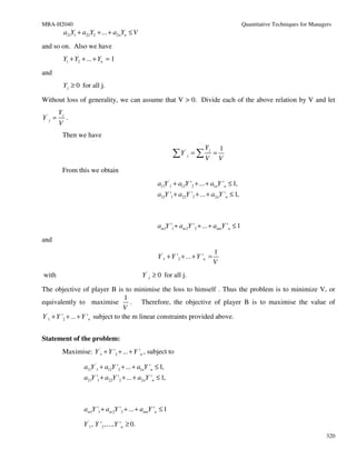
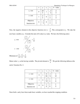
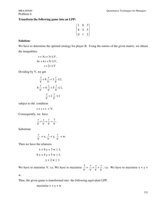
Example 1:
The arrival rate of customers at a banking counter follows a poisson distibution with a mean of 30 per hours. The service rate
of the counter clerk also follows poisson distribution with mean of 45 per hour.
a) What is the probability of having zero customer in the system ?
b) What is the probability of having 8 customer in the system ?
c) What is the probability of having 12 customer in the system ?
d) Find Ls, Lq, Ws and Wq
Solution
Given arrival rate follows poisson distribution with
mean =30
∴δ= 30 per hour
Given service rate follows poisson distribution with
mean = 45
∴µ = 45 Per hour
∴Utilization factor φ = δ/µ
= 30/45
= 2/3
= 0.67
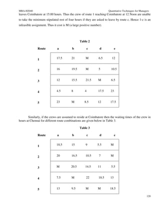
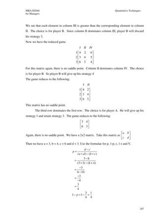
a) The probability of having zero customer in the system
P0 = φ0 (1- φ)
= 1- φ
= 1-0.67
344](https://image.slidesharecdn.com/qtformanagers-101217142149-phpapp02/85/Qualitative-Technique-for-managers-344-320.jpg)
![MBA-H2040 Quantitative Techniques for Managers
= 0.33
b) The probability of having 8 customers in the system
P8 = φ8 (1- φ)
= (0.67)8 (1-0.67)
= 0.0406 x 0.33
= 0.0134
Probability of having 12 customers in the system is
P12 = φ12 (1- φ)
= (0.67)12 (1-0.67)
= 0.0082 x 0.33 = 0.002706
Ls = φ = 0.67
1- φ 1-0.67
= 0.67 = 2.03
0.33
= 2 customers
Lq = φ2 = (0.67)2 = 0.4489
1- φ 1-0.67 0.33
= 1.36
= 1 Customer
Ws = 1 = 1 = 1
µ-δ 45-30 15
= 0.0666 hour
Wq = φ = 0.67 = 0.67
µ-δ 45-30 15
= 0.4467 hour
Example 2 :
At one-man barbar shop, customers arrive according to poisson dist with mean arrival rate of 5 per hour
and the hair cutting time was exponentially distributed with an average hair cut taking 10 minutes. It is
assumed that because of his excellent reputation, customers were always willing to wait. Calculate the
following:
(i) Average number of customers in the shop and the average numbers waiting for a haircut.
(ii) The percentage of time arrival can walk in straight without having to wait.
(iii) The percentage of customers who have to wait before getting into the barber’s chair.
Solution:-
Given mean arrival of customer δ = 5/60 =1/12
and mean time for server µ = 1/10
∴φ = δ / µ = [1/12] x 10 = 10 /12
= 0.833
(i) Average number of customers in the system (numbers in the queue and in the service station)
Ls = φ / 1- φ = 0.83 / 1- 0.83
= 0.83 / 0.17
= 4.88
= 5 Customers
(ii) The percentage of time arrival can walk straight into barber’s chair without waiting is
Service utilization =φ%
= δ / µ%
= 0.833 x 100
=83.3
345](https://image.slidesharecdn.com/qtformanagers-101217142149-phpapp02/85/Qualitative-Technique-for-managers-345-320.jpg)
![MBA-H2040 Quantitative Techniques for Managers
(v) Maximum number of customers permitted in the system is infinite
Then the steady state equation to obtain the probability of having n customers in the system is
Pn = φ n Po , o ≤n ≤C
n!
= φ n Po for n > c Where φ / c < 1
C n-c C!
Where [δ / µc] < 1 as φ = δ / µ
C-1
∴ P0 ={[Σ φn/n!] + φc / (c! [1 - φ/c])}-1
n=0
where c! = 1 x 2 x 3 x …………….. upto C
Lq = [φ c+1 / [c-1! (c - φ )] ] x P0
= (cφ Pc) / (c - φ )2
Ls = Lq +φ and Ws = Wq + 1 / µ
Wq = Lq / δ
Under special conditions Po = 1 - φ and Lq = φ C+! / c 2 Where φ <1 and
c
Po = (C-φ) (c – 1)! / c
and Lq = φ / (c-φ ), where φ / c < 1
Example 1:
At a central warehouse, vehicles are at the rate of 24 per hour and the arrival rate follows poisson distribution. The unloading
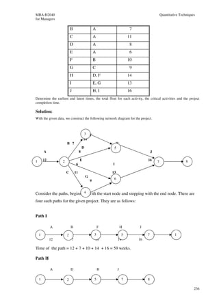
time of the vehicles follows exponential distribution and the unloading rate is 18 vehicles per hour. There are 4 unloading
crews. Find
(i) Po and P3
(ii) Lq, Ls, Wq and Ws
Solution:
Arrival rate δ = 24 per hour
Unloading rate µ = 18 Per hour
No. of unloading crews C=4
φ=δ/µ = 24 / 18=1.33
C-1
(i) P0 ={[Σ φn/n!] + φc / (c! [1 - φ/c])}-1
n=0
3
={[Σ (1.33)n/n!]+ (1.33)4 /(4! [1 - (1.33)/ 4])}-1
n=0
={ (1.33)0 / = 0! + (1.33)1 / 1! + (1.33)2 / 2! + (1.33)3 / 3! +
(1.33)4 / 24! [1 - (1.33)/ 4] }-1
=[1 + 1.33 + 0.88 + 0.39 + 3.129/16.62] -1
=[3.60 + 0.19]-1 = [3.79]-1
= 0.264
We know Pn = ( φn / n!) Po for 0≤n≤c
∴ P3 = ( φ3 / 3!) Po Since 0 ≤ 3 ≤ 4
= [(1.33)3 / 6 ] x 0.264
= 2.353 x 0.044
= 0.1035
(ii) Lq = φC+1 X P0
(C – 1)! (C-φ)2
= (1.33)5 X 0.264
3! X (4 – 1.33)2
= (4.1616) X 0.264
6 X (2.77)2
347](https://image.slidesharecdn.com/qtformanagers-101217142149-phpapp02/85/Qualitative-Technique-for-managers-347-320.jpg)
![MBA-H2040 Quantitative Techniques for Managers
= (4.1616) X 0.264
46 .0374
= 1.099 / 46.0374
= 0.0239
= 0.0239 Vehicles
Ls = Lq + φ = 0.0239 + 1.33
= 1.3539 Vehicles
Wq = Lq / δ = 0.0239 /24
= 0.000996 hrs
Ws = Wq + 1 / µ = 0.000996 + 1/18
= 0.000996 + 0.055555
= 0.056551 hours.
Example 2 :-
A supermarket has two girls ringing up sales at the counters. If the service time for each customer is exponential with mean 4
minutes and if the people arrive in poisson fashion at the rate of 10 per hour
a) What is the probability of having to wait for service?
b) What is the expected percentage of idle time for each girl?
c) If a customer has to wait, what is the expected length of his waiting time?
Solution:-
C-1
P0 ={[Σ φn/n!] + φc / (c! [1 - φ/c])}-1
n=0
Where φ = δ / µ ∴ given arrival rate = 10 per hour
δ = 10 / 60 = 1 / 6 per minute
Service rate = 4 minutes
∴µ=1/4 person per minute
Hence φ = δ / µ = (1 / 6) x 4 =2/3
= 0.67
1
P0 ={[Σ φn/n!]+(0.67)2 / (2! [1 - 0.67/2])}-1
n=0
=[1 + ( φ / 1!) ] + 0.4489 / (2 – 0.67)]-1
=[1 + 0.67 + 0.4489 / (1.33)]-1
=[1 + 0.67 + 0.34]-1
=[ 2.01]-1
=1/2
The Probability of having to wait for the service is
P (w > 0)
= φc X P0
c! [1 - φ /c]
= 0.67 2X (1 / 2)
2! [1 – 0.67 /2]
= 0.4489 / 2.66
= 0.168
b) The probability of idle time for each girl is
= 1- P (w > 0)
348](https://image.slidesharecdn.com/qtformanagers-101217142149-phpapp02/85/Qualitative-Technique-for-managers-348-320.jpg)
![MBA-H2040 Quantitative Techniques for Managers
= 1-1/3
= 2/3
∴ Percentage of time the service remains idle = 67% approximately
c) The expected length of waiting time (w/w>0)
= 1 / (c µ - δ)
= 1 / [(1 / 2) – (1 / 6) ]
= 3 minutes
Examples 3 :
A petrol station has two pumps. The service time follows the exponential distribution with mean 4 minutes and cars arrive
for service in a poisson process at the rate of 10 cars per hour. Find the probability that a customer has to wait for service.
What proportion of time the pump remains idle?
Solution: Given C=2 The arrival rate = 10 cars per hour.
∴δ = 10 / 60 = 1 / 6 car per minute
Service rate = 4 minute per cars.
Ie µ = ¼ car per minute.
φ =δ/µ = (1/6) / (1/4)
=2/ 3
= 0.67
Proportion of time the pumps remain busy
=φ/c = 0.67 / 2
= 0.33
=1/3
∴ The proportion of time, the pumps remain idle
=1 – proportion of the pumps remain busy
= 1-1 / 3 =2/3
C-1
P0 ={[Σ φn/n!] + φc / (c! [1 - φ/c])}-1
n=0
=[ ( 0.67)0 / 0!) + ( 0.67)1 / 1!) + ( 0.67)2 / 2!)[1- ( 0.67 / 2)1 ]-1
=[1 + 0.67 + 0.4489 / (1.33)]-1
=[1 + 0.67 + 0.33]-1
=[ 2]-1
=1 / 2
Probability that a customer has to wait for service
= p [w>0]
= φc x P0 = (0.67)2 x 1/2
[c [1 - φ / c] [2![1 – 0.67/2]
= 0.4489 = 0.4489
1.33x2 2.66
= 0.1688
5.2 Simulation :
Simulation is an experiment conducted on a model of some system to collect necessary information on the behaviour of that
system.
5.2.1 Introduction :
The representation of reality in some physical form or in some form of Mathematical equations
are called Simulations .
Simulations are imitation of reality.
For example :
349](https://image.slidesharecdn.com/qtformanagers-101217142149-phpapp02/85/Qualitative-Technique-for-managers-349-320.jpg)
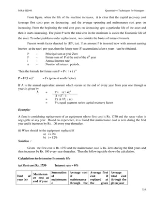

![MBA-H2040 Quantitative Techniques for Managers
first year of its operation is Rs.65,000 and it decreases by Rs.10,000 every year thereafter. Find
the economic life of the equipment by assuming the interest rate as 12%.
[Ans : Economic life = 13 years and the corresponding annual equivalent cost = Rs. 34,510]
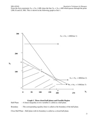
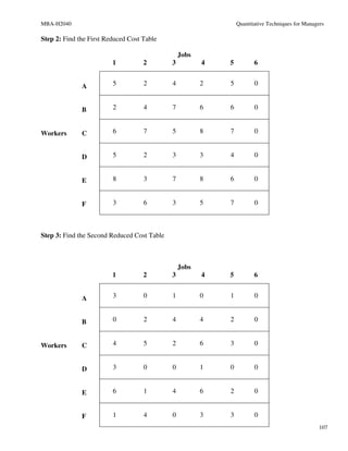
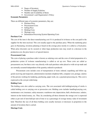
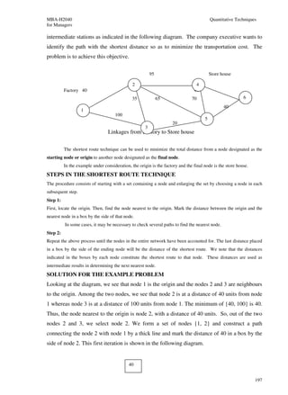
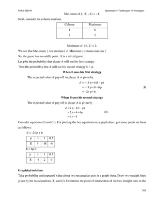
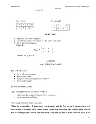
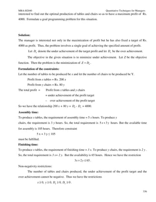
7. The following table gives the operation cost, maintenance cost and salvage value at the end of
every year of machine whose purchase value is Rs. 12,000. Find the economic life of the
machine assuming.
a) The interest rate as 0%
b) The interest rate as 15%
Operation cost at Maintenance cost Salvage value at the end
End of
the end of year at the end of year of year (Rs)
year
(Rs) (Rs)
1 2000 2500 8000
2 3000 3000 7000
3 4000 3500 6000
4 5000 4000 5000
5 6000 4500 4000
6 7000 5000 3000
7 8000 5500 2000
8 9000 6000 1000
Ans :
a) Economic life of the machine = 2 years
b) Economic life of the machine = 2 years
358](https://image.slidesharecdn.com/qtformanagers-101217142149-phpapp02/85/Qualitative-Technique-for-managers-358-320.jpg)


The document discusses the stages of development of Operations Research (OR). It describes the 6 key steps in the OR process: 1) Observe the problem environment, 2) Analyze and define the problem, 3) Develop a model, 4) Select appropriate data input, 5) Provide a solution and test its reasonableness, and 6) Implement the solution. The goal is to methodically move from defining the problem to implementing a tested solution that improves the organization's operations.