OR note.pdf

OPERATION RESEARCH MGMT 441
1 | P a g e
CHAPTER ONE: INTRODUCTION TO OPERATION RESEARCH
1.1. The history of Operation Research
Since the advent of the industrial revolution, the world has been a remarkable growth in the size
and complexity of organizations. The artisan's small shops of an earlier era have evolved into
billion- dollar corporations of today. Integral parts of this revolutionary change have been a
tremendous increase in the division of labor and segmentation of management responsibilities in
these organizations. This increasing specialization has created new problems, problems that are
still occurring in many organizations. One problem is a tendency for many components of
organizations to grow in to relatively with their own goals and value system, thereby
autonomous empires losing sight of how their activities and objectives mesh with those of the
overall organization. What is best for one component frequently is detrimental to another, so the
components may end up working at cross purposes. A related problem is that as the complexity
and specialization in an organization increase, it becomes more and more difficult to allocate the
available resources to the various activities in a way that is more effective for the organization as
a whole.
These kinds of problems and the need to find a better way to solve them provided the
environment for the emergence of operation research (OR).
The root of OR can be traced back many decades, when early attempts were made to use a
scientific approach in the management of organizations. However, the beginning of the activities
called Operation Research has generally been attributed to the military services early in World
War II. Because of the war effort, there was an urgent need to allocate scare resources to various
military operations and to the activities within each operation in an effective manner. Therefore,
the British and then the US military management called upon a large number of scientists to
apply a scientific approach to dealing with this and other strategic and tactical problems. In effect
they were asked to do research on (military) operations. These teams of scientists were the First
OR teams. By developing effective methods of using the new tool of radar, these teams were
instrumental in winning the Air battle of Britain. Through their research on how to better manage
convoy and antisubmarine operations, they also played a major role in winning the Battle of the
North Atlantic. Similar efforts assisted the Island Campaign in the Pacific.

2 | P a g e
When the war ended, the success of OR in the war effort spurred interest in applying OR outside
the military as well. As the industrial boom following the war was running its course, the
problems caused by the increasing complexity and specializations in organizations were again
coming to the forefront. It was becoming apparent to a growing number of people, including
business consultants who had served on or with the OR teams during the war, that these were
basically the same problems that had been faced by the military but in a different context. By the
early 1950s, these individuals had introduced the use of OR to a variety of organizations in
business, industry, and government. The rapid spread of OR soon followed.
At least two other factors that played a key role in the rapid growth of OR during this period can
be identified. One was the substantial progress that was made early in improving the techniques
of OR. After the war, many of the scientists who had participated on OR teams or who had heard
about this work were motivated to pursue research relevant to the field; important advancements
in the state of the art resulted. A prime example is the simplex method for solving linear
programming problems, developed by George Dantzig in 1947. Many of the standard tools of
OR, such as linear programming, dynamic programming, queuing theory, and inventory theory,
were relatively well developed before the end of the 1950s.
A second factor that gave great impetus to the growth of the field was the onslaught of the
computer revolution. A large amount of computation is usually required to deal most effectively
with the complex problems typically considered by OR. Doing this by hand would often be out
of the question. Therefore, the development of electronic digital computers, with their ability to
perform arithmetic calculations thousands or even millions of times faster than a human being
can, was a tremendous boon to OR. A further boost came in the 1980s with the development of
increasingly powerful personal computers accompanied by good software packages for doing
OR. This brought the use of OR within the easy reach of much larger numbers of people. Today,
literally millions of individuals have ready access to OR software. Consequently, a whole range
of computers from mainframes to laptops now are being routinely used to solve OR problems.
1.2. Nature and Significance of Operation Research
As its name implies, operations research involves “research on military operations. This indicates
the approach as well as the area of its applications. The operations research approach is
particularly useful in balancing conflicting objectives (goals or interest) where there are many

3 | P a g e
alternative courses of action available to decision makers. In a theoretical sense, the optimum
decision must be one that is best for the organization as a whole. It is often called the global
optimum. A decision that is best for one or more sections of the organization is usually called
suboptimum decision. The OR approach attempt to find global optimum by analyzing inter-
relationships among the system components involved in the problem. One such situation is
described below.
Consider a large organization with a number of management specialists but not necessarily
well coordinated. For example, consider the basic problem of maintaining stock of finished
goods. To marketing manager, stocks of a large variety of products are a means of supplying the
company's customers with what they want and when they want it. Clearly, according to
marketing manager, a fully stocked warehouse is of prime importance to the company. But the
production manager argues for long production runs preferably on smaller product range,
particularly if significant time is lost when production is switched from one variety to another.
The result would gain be a tendency to increase the amount of stock carried but it is, of course,
vital that the plant should be kept running. On the other hand, the finance manager sees stocks in
terms of capital tied up unproductively and argues strongly for their reduction. Finally, there
appears the personnel manager for whom a steady level of production is advantageous for having
better labor relations. Thus, all these people would claim to uphold the interests of the
organization, but they do so only from their specialized point of view. They may come up with
contradictory solutions and obviously, they cannot all be right.
In view of the above involving the whole system, the decision makers, whatever his
specialization, will need help and it is in the attempt to provide his assistance that OR has been
developed. Operation research attempts to resolve the conflicts of interest among various
sections of the organization and seeks the optimal solution which may not be acceptable to one
department but is in the interest of the organization as a whole. Further, OR is concerned with
providing the decision maker with decision aids (or rules) derived from:
i. A total system orientation,
ii. Scientific methods of investigation, and
iii. Models of reality, generally based on quantitative measurement and techniques.
Thus, successful application of OR techniques for solving a problem must involve the following steps.

4 | P a g e
1. Constructing mathematical, economic or statistical model of the problem under study to treat
situations of complexity and uncertainty. This helps to view the problem in its entirety.
2. Analyzing the relationship among different variables and/or parameters associated with the
problem, so as to determine consequences of decision alternatives.
3. Suggesting suitable measures of desirability (effectiveness or objective function) in order to
evaluate the relative merit of decision alternatives (course of action, acts or strategies).
Remark: A system is defined as an arrangement of components designed to achieve a particular
objective(s) according to plan. The components may be either physical or conceptual or both but
they share a unique relationship with each other and with the overall objective of the system.
Thus, operations research is applied to problems that concern how to conduct and coordinate the
operations (i.e., the activities) within an organization. The nature of the organization is
essentially immaterial, and, in fact, OR has been applied extensively in such diverse areas as
manufacturing, transportation, construction, telecommunications, financial planning, health care,
the military, and public services, to name just a few. Therefore, the breadth of application is
unusually wide.
1.3. Features of Operation Research
The features of operation research approach to any decision and control problem can be
summarized as under.
1.3.1. Interdisciplinary Approach.
Interdisciplinary teamwork is essential because while attempting to solve a complex
management problem, one person may not have a complete knowledge of all aspects (such as
economic, social, political, psychological, engineering, etc.). This means we should not expect a
desirable solution to managerial problems. Therefore, a group of individuals specializing in
mathematics, statistics, economics, engineering, computer science, psychology, etc. can be
organized so that each aspect of the problem could be analyzed by a particular specialist in that
field in order to arrive at an appropriate and desirable solution of the problem. However, there
are certain situations which may be analyzed even by one individual.
1.3.2. Methodological Approach
Operation research is a scientific methods, techniques and tools to problems solving the
operations of systems so as to provide those in control of operations with optimum solution to
the problems. The scientific method consists of observing, and defining the problem; formulating

5 | P a g e
and testing the hypothesis; and analyzing the result of the test. The data so obtained is then used
to decide whether the hypothesis should be accepted or not. If the hypothesis is accepted, the
result should be implemented. Otherwise an alternative hypothesis has to be formulated.
1.3.3. Wholistic Approach
While arriving at a decision, an operation research team examines the relative importance of all
conflicting and multiple objectives and the validity of claims of various departments of the
organization from the perspective of the whole.
1.3.4. Objectivistic Approach
An operation research approach seeks to obtain an optimal solution to the problem under
analysis. For this, a measure of desirability (or effectiveness) is defined, based on the
objective(s) of the organization. A measure of desirability so defined is then used to compare
alternative courses of action with respect to their outcomes.
DEFINING OPERATIONS RESEARCH:
OPERATIONS RESEARCH has been defined in various ways and it is perhaps too early to
define it in some authoritative way. However, given below are a few opinions about the
definition of OR which have been changed along-with the development of the subject.
In 1946 Morse & Kimbel has defined as;
"OR is a scientific method of providing executive departments with a quantitative basis for
decision regarding the operations under their control"
In 1948 Blackett defined as;
"OR is a scientific method of providing executives with any analytical and objective basis for
decisions"
Another definition is due to Morse who defined in 1948 as;
"The term OR, has here-to fore been used to connote various attempts to study operations of war
by scientific methods. From a more general point of view, OR can be considered to be an attempt
to study those operations of modern society which involved organizations of men or men and
machines".
Later on in 1957, Churchmen Ackoff and Arnoff defined;
"OR is the application of scientific methods, techniques and tools to problems involving the
operations of systems so as to provide those in control of the operations with optimum solutions
to the problem".

6 | P a g e
In 1958 Saaty defined OR as; "The art of giving bad answer to problems to which, otherwise,
worse answers are given".
The Operational Research Society of U.K. defines OR as: “Operational Research is the
application of the methods of science to complex problems arising in the direction and
management of large systems of men, machines, materials and money in industry, business,
government and defense.
The distinctive approach is to develop a scientific model of the system, incorporating
measurements of factors, such as chance and risk, with which to compare the outcome of
alternative decisions, strategies and controls. The purpose is to help management determine its
policies and actions scientifically."
In the USA, where it is called Operations Research, the OR Society of America says more
briefly;
"OR is concerned with scientifically deciding how to best design and operate man-machine
systems, usually under conditions requiring the allocation of scarce resources".
An even briefer definition might be "Science applied to management", but however, it might be
defined, there is no doubt that OR provides the numerate scientist - of whatever discipline-with
an opportunity to apply the skills of science in the field of Management.
Before proceeding further let us define for the sake of clarity some fundamental terms.
MANAGEMENT, MANAGEMENT SCIENCE AND OR:
MANAGEMENT may be equated with decision-making and control. Government ministers
manage the economy industrialists make decision within their companies and individual make
personal decisions.
MANAGEMENT SCIENCE is the study of problems as abstractions and the application of the
resulting theory to practical situations. Its two fundamental disciplines are behavioral science and
science and quantitative methods.
OPERATIONS RESEARCH (OR) is the application of quantitative methods to decision making.
It formulates problems incisively (clearly and effectively) and assesses the possible consequence
of alternative course of action, so that informed and effective decisions can be taken.
Scientific Method in Operations Research

7 | P a g e
The most important feature of operation research is the use of the scientific method and building
of decision models. There are three phases of the scientific method on which OR approach is
based.
1. Judgment phase
This phase includes:
(i) identification of the real-life problem,
(ii) selection of the appropriate objective and the values of various variables related to this
objective,
(iii) application of the appropriate scale of measurement, i.e. deciding the measure of
effectiveness (desirability) and
(iv) formulation of an appropriate model of the problem, abstracting the essential information, so
that a solution to the decision maker’s goals can be obtained.
2. Research phase
This phase is the largest and longest among other two phases. However, the remaining two are
also equally important as they provide the basis for a scientific method. This phase utilizes: (i)
observation and data collection for a better understanding of the problem, (ii) formulation of the
hypothesis and model, (iii) observation and experimentation to test the hypothesis on the basis of
additional data, (iv) analysis of the available information and verification of the hypothesis using
pre-established measures of desirability, (v) prediction of various results from the hypothesis,
and (vi) generation of the result and consideration of alternative methods.
3. Action phase
This phase consists of making recommendations for implementing the decision by an individual
who is in the position to implement results. This individual must be aware of the environment in
which the problem occurred, objective, assumptions and omissions of the model of the problem.
1.4. MODELS AND MODELING IN OPERATION RESEARCH

8 | P a g e
OR APPROACH TO PROBLEM SOLVING:
OR encompasses a logical systematic approach to problem solving. This approach to problem
solving as shown below and follows a generally recognized ordered set or steps:
(1) Observation,
(2) Definition of the problems,
(3) Model construction,
(4) Model solution, and
(5) Implementation of solution results.
1. Observation
The first step in a problem-solving exercise in OR is the identification of a problem that exists in
the system. This requires that the system be continuously and closely observed so that problems
can be identified as soon as they occur.
2. Definition of the Problem
Once it has determined that a problem exists, it must be clearly and concisely defined.
The problem definition includes the limits of the problems and the degree to which it pervades
other organs of the system. A requirement of problem definition is that the goals (or objective)
Must be clearly defined which helps to focus attention on what the problem is.
3. Model Construction
An OR model is an abstract representation of an existing problem situation. It can be in the form
of a graph or chart, but mostly, an OR model consists of a set of mathematical relationship. In
OR terminology, these are called objective function and constraints.
4. Model Solution
Once models are constructed, they are solved using the OR techniques, presented in the next
section. Actually, it is difficult to separate model construction and solution in most cases, since
OR technique usually applies to a specific type of model. Thus, the model type and solution
method are both part of the OR technique.
5. Implementation of Results

9 | P a g e
The results of an OR technique is information which helps in making a decision. The beauty of
OR process lies in obtaining, the results which are implement able or we call it a feasible whole
exercise will go waste.
OR is an On-going Process
Once the five steps described above are completed, it does not necessarily mean that OR process
is completed. The model results and the decisions based on the results provide feedback to the
original model. The original OR model can be modified to test different conditions and decisions
that might occur in the future. The results may indicate that a different problem exists that had
not been thought of previously, thus the original model is altered or reconstructed. As such, the
OR process is continuous rather than simply consisting of one solution to one problem.
Operations Research Techniques:
Two of the five steps of OR process, model construction and solution, encompass the actual use
of OR techniques. These techniques can be loosely classified into five categories.
1) Linear mathematical programming technique consist of first, identifying problem as being
solvable by linear programming; second formulation of unturned problem and then finding the
solution by using established mathematical techniques. It derives its name from the fact that the
functional relationship in the mathematical model are linear and the solution techniques consists
of a predetermined mathematical step i.e. program.
2) Probabilistic techniques cover those problems in which all parameters are not known with
certainty. The solution results are assumed to be known with uncertainty, with probability that
other solution might exist.
3) Inventory techniques are specifically designed for the analysis of inventory problem
frequently encountered by the business firms. This particular business function is singled out for
attention, since it typically represents a significant area of cost for almost every business. This
category is divided into probabilistic and deterministic techniques.
4) Network techniques consist of models that are represented by diagrams rather than strictly
mathematical relationship i.e. pictorial representation of the system under consideration.
These models can represent either probabilistic or deterministic systems.
5) Other techniques consist of all the remaining techniques, which do not come under the four
heads mentioned above. For example, Dynamic programming employs a different modeling and
solution logic than linear programming. In non-linear programming either the objective function

10 | P a g e
or the constraints or both can be non-linear functions, which would require altogether different
solution technique.
USES OF OPERATIONS RESEARCH
In its recent years of organized development, OR has entered successfully many different areas
of research for military government and industry in many countries of the world.
The basic problem in most of the developing countries in Asia and Africa is to remove poverty
and improve the standard of living of a common man as quickly as possible. So there is a great
scope for economists, statisticians, administrators, politicians and the technicians working in a
team to solve this problem by an OR approach. The possible application sectors, in Pakistan, are
as under:-
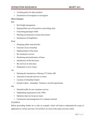
1) Macro Economic Planning:
OR can be employed for Macro-Economic Planning of the country:
a) Input / Output Analysis: by using LP models. This input/output analysis can be of any
duration [i.e. of short term (up to say 10 years)-Five Year Plan; and of long term (10-30 years)].
b) Investment Planning: OR can be employed in the Investment Planning of the country where
investment plans for the next five or ten years are prepared. Mixed Integer Programming and
Linear Programming techniques can be used.

11 | P a g e
c) Choice of Projects: OR can help the people in the planning in choosing the optimal project.
This sort of choice would need Integer Programming and Quadratic Assignment techniques.
d) OR can also be used in Simulation Modeling of the Economy of the country.
2) Sectoral Planning:
OR can also be employed in a particular sector of the Economy, e.g. in agriculture, in finance, in
industry, in marketing, in production, in management etc.
a) Scheduling all operations within a sector can be done by using OR e.g. production scheduling
+ Distribution planning + marketing + Personnel management + maintenance + ...............
b) Schedule of some operations within a sector can be done by employing OR e.g. Inventory
planning in agriculture or distribution of fertilizer etc.
3) Micro Economic Planning:
This sort of activity involve for example:
 Planning the operations of a Company.
 Improving the layout of a workshop in a company.
 Finding size of a hospital in an area etc.
There is a great potential for utilizing OR in this area of planning in our country.
POTENTIAL AREAS OF APPLICATIONS
As mentioned earlier OR can be applied in every field of life. Here are few of the many fields
where OR has potential application. This list is by no means comprehensive or exhaustive but
definitely will provide an idea of the power of OR as a separate discipline.
Operations Research in the Public Sector
Federal, Provincial and Local Government
• Development of Country Structure Plans
• Manpower Planning and Career Development in Govt. Departments
• Organization of Long-Term planning groups at the National Level
• Corporate Planning in Local Government
• Allocation of Government Houses
• Estimation of Future Requirement of School/College Building
• Placing of Fire Brigade in a City
• Measuring the Effectiveness of Police
• Timetabling in Schools and Colleges for Efficient use of Space

12 | P a g e
Health
• Management policies for 120-bed nursing units
• Optimum size of general hospitals
• Appointment systems for hospital outpatients
• Stock control for regional and area health units
• National and area planning of health services
• Manpower planning for nurses, radiographers, etc.
• Commissioning of a new general hospital
• Simulation of pathology laboratories
• Organizing an ambulance service
• Care provided by community nurses
Defense
• Arms control and disarmament studies
• Communications network development
• Logistic support in operations
• Field experimentation
• War games and other models of battle
• Equipment procurement
• Reinforcement and redeployment problems
Operations Research in Industry & Commerce
Finance and Investment
• Developing the five-year plan for a food manufacturer
• Development of the pipeline
• Computer based financial planning
• Portfolio selection
• Structure for the assets of a bank
• Evaluating investment in a new plant
• Corporate planning in the chemical industry
• Financing expansion of a small firm
Production
• Production scheduling in a steel works

13 | P a g e
• Meeting peak demands for electricity
• Minimization of costs of power station maintenance
• Scheduling newsprint deliveries
• Stock levels of steel plate
• Meeting seasonal demands for products
• Blending scrap metals
• Stock policy for a paint manufacturer
• Allowing for yarn breaks in spinning
• Meeting customer requirements for carpets
• Planning a quarry's output
• Optimum layout for belt coal transport in a colliery
Marketing
• Launching a new product
• Advertising effectiveness and cost
• Planning sales territories
• Measurement of consumer loyalty
• Buyer-seller behavior
• Advertising research and media scheduling
• Most profitable retail brand mix
• Developing customer service policies
• Pricing policies for confectionery
Personnel
• Personnel shift planning
• Manpower planning
• Manpower for an assembly line
• Effects of flexible working hours
Distribution
• Distribution of Products.
• Returnable bottles: how many?
• Refinery crude tank capacity
• Depot location of pharmaceutical products

14 | P a g e
• Trucking policy for dairy products
• Distribution of newspapers to newsagents
OR in Transport
Rail
• Rail freight management
• Required fleet size of locomotives and rolling stock
• Forecasting passenger traffic
• Planning reconstruction of main-line termini
• Introduction of freightliners
Road
• Designing urban road networks
• Forecasts of car ownership
• Implementation of bus lanes
• Re-routing bus services
• Purchasing and maintenance of buses
• Introduction of flat-fare buses
• Bus services in rural areas
• Preparation of crew rosters
Air
• Planning the introduction of Boeing 737/Airbus 300
• Allocation of aircraft and crew to routes
• Location of Islamabad Airport
• Karachi-Lahore - Islamabad - Peshawar: aircraft requirements
Sea
• Potential traffic for new container services
• Shipbuilding requirement in the 1990's
• Optimum ship size for given routes
• Construction and management of a container terminal
EXAMPLE
Before proceeding further let us take an example, which will help to understand the scope of
application in various activities. Given below are some of the major activities which

15 | P a g e
OPERATIONS:
1) Oil production from fields
2) Transportation of Crude
• from fields to refineries
• from fields to export ports (Jetties)
• from import ports (Jetties) to refineries
3) Storage of Crude
• on fields
• at Ports
• at refineries
4) Refinery Scheduling
• Operation of CDU's
• Operation of Blending Units
5) Storage of Distilled Blended Products
• at refineries
• at Jetties
• at distribution points
6) Transportation of Products
• from Jetties to refineries
• from one refinery to another for another processing
• From refinery to bulk distribution pts.
• From bulk distribution points to final consumers.
At all the stages from oil production from fields to its transportation to the final consumer
OR has been employed in the developed countries of the world. Applying on macro level is not
an easy job. This would require true and factual data computing power and trained professionals,
and perhaps at this stage we may face some problem due to limited resources in term of
manpower, money and machines, but it does not mean that we should not make a beginning.

16 | P a g e
CHAPTER TWO: LINEAR PROGRAMMING
2.1. INTRODUCTION TO LINEAR PROGRAMMING
The development of linear programming has been ranked among the most important scientific
advances of the mid-20th century, and we must agree with this assessment. Its impact since just
1950 has been extraordinary. Today it is a standard tool that has saved many thousands or
millions of dollars for most companies or businesses of even moderate size in the various
industrialized countries of the world; and its use in other sectors of society has been spreading
rapidly. A major proportion of all scientific computation on computers is devoted to the use of
linear programming. What is the nature of this remarkable tool, and what kinds of problems does
it address?
You will gain insight into this topic as you work through subsequent examples. However, a
verbal summary may help provide perspective.
Briefly, the most common type of application involves the general problem of allocating limited
resources among competing activities in a best possible (i.e., optimal) way. More precisely, this
problem involves selecting the level of certain activities that compete for scarce resources that
are necessary to perform those activities. The choice of activity levels then dictates how much of
each resource will be consumed by each activity. The variety of situations to which this
description applies is diverse, indeed, ranging from the allocation of production facilities to
products to the allocation of national resources to domestic needs, from portfolio selection to the
selection of shipping patterns, from agricultural planning to the design of radiation therapy, and
so on. However, the one common ingredient in each of these situations is the necessity for
allocating resources to activities by choosing the levels of those activities.
Linear programming uses a mathematical model to describe the problem of concern.
The adjective linear means that all the mathematical functions in this model are required to be
linear functions. The word programming does not refer here to computer programming; rather, it
is essentially a synonym for planning. Thus, linear programming involves the planning of
activities to obtain an optimal result, i.e., a result that reaches the specified goal best (according
to the mathematical model) among all feasible alternatives.
Although allocating resources to activities is the most common type of application, linear
programming has numerous other important applications as well. In fact, any problem whose

17 | P a g e
mathematical model fits the very general format for the linear programming model is a linear
programming problem. Furthermore, a remarkably efficient solution procedure, called the
simplex method, is available for solving linear programming problems of even enormous size.
These are some of the reasons for the tremendous impact of linear programming in recent
decades.
A Standard Form of the Model
We can now formulate the mathematical model for this general problem of allocating resources
to activities. In particular, this model is to select the values for x1, x2. . . xn so as to
Maximize Z =c1x1 + c2x2 +………….. +cnxn
Subject to the restrictions
a11x1 +a12x2 +………………..+ a1nxn ≤ b1
a21x1 +a22x2 +………………..+a2nxn ≤ b2
.
.
.
am1x1 +am2x2+………………. + amnxn ≤ bm,
TABLE 2.1 Data needed for a linear programming model involving the allocation of resources to
activities
Resource Usage per Unit of Activity Sign of
equalities
Amount of
Resources
Available
Resources Activity
Contribution
to Z per unit
of activity
C1 C2 . . . Cn
1 2 . . . n
1 a11 a 12 . . . a 1n ≤ = ≥ b1
2 a21 a22 . . . a2n ≤ = ≥ b2
. . . . . . . . .
. . . . . . . . .
m am1 am2 . . . amn ≤ = ≥ bm
And
X1 ≥0, x2 ≥ 0, . . . , xn ≥0.

18 | P a g e
We call this our standard form1 for the linear programming problem. Any situation whose
mathematical formulation fits this model is a linear programming problem.
Common terminology for the linear programming model can now be summarized.
The function being maximized, c1x1 +c2x2+………+ cjxn, is called the objective function.
The restrictions normally are referred to as constraints. The first m constraints (those with a
function of all the variables ai1x1 +ai2x2 +…………..+ ainxn on the left-hand side) are sometimes
called functional constraints (or structural constraints). Similarly, the xn ≥ 0 restrictions are
called non-negativity constraints (or non-negativity conditions).
2.1.1. Concept and Importance of Linear Programming
Linear Programming- is an optimization method, which shows how to allocate scarce resources
such as money, materials or time and how to do such allocation in the best possible way subject
to more than one limiting condition expressed in the form of inequalities and/or equations.
It enables users to find optimal solution to certain problems in which the solution must satisfy a
given set of requirements or constraints.
Optimization in linear programming implies either maximization (such as profit, revenue, sales,
and market share) or minimization (such as cost, time, and distance) a certain objective function.
It implies that in LP we cannot max/min two quantities in one model. It involves linearly related
multi-variate functions, i.e., functions with more than one independent variable.
The goal in linear programming is to find the best solution given the constraints imposed by the
problem; hence the term constrained optimization.
2.1.2. Structure Linear programming Models (LPM)
Linear Programming (LP) models are mathematical representations of LP problems. Some LP
models have a specialized format, whereas others have a more generalized format. Despite this,
LP Models have certain characteristics in common. Knowledge of these characteristics enables
us to recognize problems that are amenable to a solution using LP models and to correctly
formulate an LP model. The characteristics can be grouped into two categories: Components and
Assumptions: The components relate to the structure of a model, whereas the assumptions reveal
the conditions under which the model is valid.
Components Assumptions
1. Objective function 1. Linearity
2. Decision variables Model 2. Divisibility Model Validity

19 | P a g e
3. Constraints Structure 3. Certainty
4. Parameters & RHSV 4. Non-negativity
Components of LP model
1. The Objective Function- is the mathematical or quantitative expression of the objective of the
company/model. The objective in problem solving is the criterion by which all decisions are
evaluated. In LPMs a single quantifiable objective must be specified by the decision maker. For
example, the objective might relate to profits, or costs, or market share, but to only one of these.
Moreover, because we are dealing with optimization, the objective will be either maximization
or minimization, but not both at a time.
2. The Decision Variables - represent unknown quantities to be resolved for. These decision
variables may represent such things as the number of units of different products to be sold, the
amount of Birr to be invested in various projects, the number of ads to be placed with different
media.
Since the decision maker has freedom of choice among actions, these decision variables are
controllable variables.
3. The constraints - are restrictions which define or limit the feasibility of a proposed course of
action. They limit the degree to which the objective can be pursued.
Atypical restriction embodies scarce resources (such as labor supply, raw materials, production
capacity, machine time, storage space), legal or contractual requirements (e.g. Product standards,
work standards), or they may reflect other limits based on forecasts, customer orders, company
policies etc.
4. Parameters - are fixed values that specify the impact that one unit of each decision variable will
have on the objective and on any constraint, it pertains to as well as to the numerical value of
each constraint.
 The components are the building blocks of an LP model. We can better understand their
meaning by examining a simple LP model as follows.
Example:
Maximize: 4X1 + 7X2 + 5X3 (Profit) ___________________ objective function
Subject to:

20 | P a g e
2X1 + 3X2 + 6X3  300 labor hrs
5X1 + X2 + 2X3  200 lb raw material A System constraints
3X1 + 5X2 + 2X3  360
X1 = 30 Individual constraints
X2  40
X1, X2, X3  0  Non-negativity constraints.
System constraints – involve more than one decision variables.
Individual constraints – involve only one decision variable.
None-negativity constraints specify that no variable will be allowed to take on a negative value.
The non-negativity constraints typically apply in an LP model, whether they are explicitly stated
or not.
Assumption of LP Models
1. Linearity. The linearity requirement is that each decision variable has a linear impact on the
objective function and in each constraint in which it appears. Following the above example,
producing one more unit of product 1 adds Br. 4 to the total profit. This is true over the entire
range of possible values of X1. The same applies to each of the constraints. It is required that the
same coefficient (from example, 2 lb. per unit) apply over the entire range of possible value so
the decision variable.
2. Divisibility. The divisibility requirement pertains to potential values of decision variables. It is
assumed that non-integer values are acceptable. For example: 3.5TV sets/hr would be acceptable
 7 TV sets/2hrs.
3. Certainty. The certainty requirement involves two aspects of LP models.
i) With respect to model parameters (i.e., the numerical values) – It in assumed that these
values are known and constant e.g. in the above example each unit of product 1 requires
2lab his is known and remain constant, and also9 the 300 lab/hr available is deemed to
be known and constant.
ii) All the relevant constraints identified and represented in the model are as they are.
4. Non-negativity. The non-negativity constraint is that negative values of variables are
unrealistic and, therefore, will not be considered in any potential solution; only positive
values and zero will be allowed.

21 | P a g e
2.3. Formulating LP Models
Once a problem has been defined, the attention of the analyst shifts to formulating a model. Just
as it is important to carefully define a problem, it is important to carefully formulate the model
that will be used to solve the problem. If the LP model is ill formulated, ill-structured, it can
easily lead to poor decisions.
Formulating linear programming models involves the following steps:
1. Define the problem/problem definition
* To determine the # of type 1 and type 2 products to be produced per month so as to
maximize the monthly profit given the restrictions.
2. Identify the decision variables or represent unknown quantities
* Let X1 and X2 be the monthly qualities of Type 1 and type 2 products
3. Determine the objective function
* Once the variables have been identified, the objective function can be specified. It is
necessary to decide if the problem is maximization or a minimization problem and the
coefficients of each decision variable.
Note: a. the units of all the coefficients in the objective function must be the
same. E.g. If the contribution of type 1 is in terms of Br so does for type 2.
b. All terms in the objective function must include a variable each term
have to have 1 variable.
c. All decision variables must be represented in the objective function.
4. Identifying the constraints
- System constraints: - more than one variable
- Individual constraints: - one variable
- Non-negative constraints
Example
1. A firm that assembles computer and computer equipment is about to start production of two new
microcomputers. Each type of micro-computer will require assembly time, inspection time and
storage space. The amount of each of these resources that can be devoted to the production of
microcomputers is limited. The manager of the firm would like to determine the quantity of each

22 | P a g e
microcomputer to produce in order to maximize the profit generated by sales of these
microcomputers.
Additional information
In order to develop a suitable model of the problem, the manager has met with design and
manufacturing personnel. As a result of these meetings, the manger has obtained the following
information:
Type 1 Type 2
Profit per unit Birr 60 Birr 50
Assembly time per unit 4hrs 10hrs
Inspection time per unit 2hrs 1hr
Storage space per unit 3cubic ft 3cubic ft
The manager also has acquired information on the availability of company resources. These
weekly amounts are:
Resource Resource available
Assembly time 100hrs
Inspection time 22hrs
Storage space 39 cubic feet
The manger also meet with the firm’s marketing manager and learned that demand for the
microcomputers was such that whatever combination of these two types of microcomputer is
produced, all of the output can be sold.
Required: Formulate the Linear programming model.
Solution:
Step 1: Problem Definition
- To determine the number of two types of microcomputers to be produced (and
sold) per week so as to maximize the weekly profit given the restriction.
Step 2: Variable Representation
- Let X1 and X2 be the weekly quantities of type 1 and type 2 microcomputers,
respectively.
Step 3: Develop the Objective Function
Maximize Z or max Z = 60X1 + 50X2
Step 4: Constraint Identification

23 | P a g e
System constraints: 4X1 + 10X2  100hrs Assembly time
2X1 + X2  22hrs inspector time
3X1 + 3X2  39 cubic feet Storage space
Individual constraint No
Non-negativity constraint X1, X2  0
In summary, the mathematical model for the microcomputer problem is:
Max Z = 60X1 + 50X2
Subject to: 4X1 + 10X2  100
2X1 + X2  22
X1 + 3X2  39
X1, X2  0
2. An electronics firm produces three types of switching devices. Each type involves a two-step
assembly operation. The assembly times are shown in the following table:
Assembly time per Unit (in minutes)
Section #1 Section #2
Model A 2.5 3.0
Model B 1.8 1.6
Model C 2.0 2.2
Each workstation has a daily working time of 7.5 hrs. The manager wants to obtain the greatest
possible profit during the next five working days. Model A yields a profit of Birr 8.25 per unit,
Model B a profit of Birr 7.50 per unit and Model C a profit of Birr 7.80 per unit. Assume that the
firm can sell all it produces during this time, but it must fill outstanding orders for 20 units of
each model type.
Required: Formulate the linear programming model of this problem.
Solution:
Step 1. Problem definition
To determine the number of three types of switching devices to be produced and sold for
the next 5 working days so as to maximize the 5 days profit.
Step 2. Variable representation

24 | P a g e
Let X1, X2 and X3 be the number of Model A, B and C switching devices respectively,
to be produced and sold.
Step 3. Develop objective function
Max Z: 8.25X1 + 7.50X2 + 7.80X3
Step 4. Constraint identification
2.5X1 + 1.8X2 + 2.0X3  2250 minutes Ass. time station 1 System
3.0X1 + 1.6X2 + 2.2X3  2250 minutes Ass. time station 2
X1  20 Model A
X2  20Model B Individual constraint
X3  20 Model C
X1, X2, X3 0 Non negativity
In summary:
Max Z: 8.25X1 + 7.50X2 + 7.80X3
subject to
2.5X1 + 1.8X2 + 2.0X3  2250 minutes
3.0X1 + 1.6X2 + 2.2X3  2250 minutes
X1  20 model A
X2  20 model B
X3  20 model C
X1, X2, X3  0 non negativity
3. A diet is to include at least 140 mgs of vitamin A and at least 145 Mgs of vitamin B. These
requirements are to be obtained from two types of foods: Type 1 and Type 2. Type 1 food
contains 10Mgs of vitamin A and 20mgs of vitamin B per pound. Type 2 food contains 30mgs of
vitamin A and 15 mgs of vitamin B per pound. If type 1 and 2 foods cost Birr 5 and Birr 8 per
pound respectively, how many pounds of each type should be purchased to satisfy the
requirements at a minimum cost?
Vitamins
Foods A B
Type 1 10 20

25 | P a g e
Type 2 30 15
Solution:
To determine the pounds of the two types of foods to be purchased to make the diet at a
minimum possible cost within the requirements.
Step 2. Variable representation
Let X1 and X2 be the number of pounds of type 1 and type 2 foods to be purchased,
respectively.
Step 3. Objective function
Min Z: 5X1 + 8X2
4. Constraints
10X1 + 30X2  140 System constraints
20X1 + 15X2  145
X1, X2  0 non-negativity constraints.
4. A farm consists of 600 hectares of land of which 500 hectares will be planted with corn, barley
and wheat, according to these conditions.
(1) At least half of the planted hectare should be in corn.
(2) No more than 200 hectares should be barley.
(3) The ratio of corn to wheat planted should be 2:1
It costs Birr 20 per hectare to plant corn, Birr 15 per hectare to plant barley and Birr 12 per
hectare to plant wheat.
Required: Formulate this problem as an LP model that will minimize planting cost while
achieving the specified conditions.
Solution:
To determine the number of hectares of land to be planted with corn, barley and wheat at
a minimum possible cost meeting the requirements.
Step 2. Decision variable representation

26 | P a g e
Let X1 be the number of hectares of land to be planted with corn, X2 be the number of
hectares of land to be planted with barley, and X3 be the number of hectares of land to
be planted with wheat.
Step 3. Objective function
Min Z = 20X1 + 15X2 + 12X3
Step 4. Constraints
X1 + X2 + X3 = 500
X1  250
X2  200
X1 – 2X2 = 0
X1, X2, X3  0
In summary
Min Z: 20X1 + 15X2 + 12X3
: X1 + X2 + X2 = 500
X1 – 2X2 = 0
X1  250
X2  200
X1, X2, X3  0
ADDITIONAL EXAMPLES WITH THE PROPER LP MODEL FORMULATION
Example 1. Ingredients Mixing
Fauji Foundation produces a cereal SUNFLOWER, which they advertise as meeting the
minimum daily requirements for vitamins A and D. The mixing department of the company uses
three main ingredients in making the cereal-wheat, oats, and rice, all three of which contain
amounts of vitamin A and D. Given that each box of cereal must contain minimum amounts of
vitamin A and D, the company has instructed the mixing department determine how many
ounces of each ingredient should go into each box of cereal in order to minimize total cost.
This problem differ Br from the previous one in that its objective is to minimize cost, rather than
maximize profit.
Each ingredient has the following vitamin contribution and requirement per box.
Vitamin Contribution

27 | P a g e
Vitamin Wheat (mg./oz) Oats (mg./oz) Rice (mg./oz.) Milligrams
Required/Box
A 10 20 08 100
D 07 14 12 70
The cost of one ounce of wheat is Br. 0.4, the cost of an ounce of oats is Br. 0.6, and the cost of
one ounce of rice is Br. 0.2.
Solution:
Decision Variables
This problem contains three decision variables for the number of ounces of each ingredient in a
box of cereal:
X1 = ounces of wheat
X2 = ounces of oats
X3 = ounces of rice
The Objective Function
The objective of the mixing department of the Fauji Foundation is to minimize the cost of each
box of cereal. The total cost is the sum of the individual costs resulting from each ingredient.
Thus, the objective function that is to minimize total cos, Z, is expressed as
Minimize Z = Br. 0.4X1 + 0.6X2 + 0.2X3
Where Z = total cost per box
Br. 0.4 X1 = cost of wheat per box
Br.0.6 X2 = cost of rice per box
Br.0.2 X3 = cost of rice per box
Model Constraints
In this problem the constraints reflect the requirements for vitamin consistency of the cereal.
Each ingredient contributes a number of milligrams of the vitamin to the cereal. The constraint
for vitamin A is
10 X1 + 20 X2 + 8 X3 ≥ 100 milligrams
Where
10 X1 = vitamin A contribution (in mg.) for wheat
20 X2 = vitamin A contribution (in mg.) for oats
8X3 = vitamin A contribution (in mg.) for rice

28 | P a g e
Notice that rather than an (≤) inequality, as used in the previous example; this constraint requires
a ≥ (greater than or minimum requirement specifying that at least 100 mg of vitamin A must be
in a box. If a minimum cost solution results so that more than 100 mg is in the cereal mix, which
is acceptable, however, the amount cannot be less than 100 mg.
The constraint for vitamin D is constructed like the constraint for vitamin A.
7X1 + 14 X2 + 12X3 ≥ 70 milligrams
As in the previous problem there are also nonnegative constraints indicating that negative
amounts of each ingredient cannot be in the cereal.
X1, X2, X3 ≥0
The L.P. model for this problem can be summarized as
Minimize Z = Br. 0.4 X1 + 0.6 X2 + 0.2 X3
Subject to
10X1 + 20 X2 + 8X3 ≥100
7 X1 + 14 X2 + 12 X3 ≥ 70
X1, X2, X3 ≥ 0
Example2. Investment Planning
Mr. Majid Khas has Br. 70, 000 to investment in several alternatives. The alternative investments
are national certificates with an 8.5% return, Defense Savings Certificates with a 10% return,
NIT with a 6.5% return, and khas deposit with a return of 13%. Each alternative has the same
time until maturity. In addition, each investment alternative has a different perceived risk thus
creating a desire to diversify. Magid Khas wants to know how much to invest in each alternative
in order to maximize the return.
The following guidelines have been established for diversifying the investments and lessening
the risk;
1. No more than 20% of the total investment should be in khas deposit.
2. The amount invested in Defense Savings Certificates should not exceed the amount invested
in the other three alternatives.
3. At least 30% of the investment should be in NIT and Defense Savings Certificates.
4. The ration of the amount invested in national certificates to the amount invested in NIT should
not exceed one to three.

29 | P a g e
Solution:
Decision Variables
There are four decision variables in this model representing the monetary amount invested in
each investment alternative.
X1 = the amount (Br.) invested in national certificates
X2 = the amount (Br.) invested in Defense Savings Cert.
X3 = the amount (Br.) invested in NIT.
X4 = the amount (Br.) invested in khas deposit.
The objective of the investor is to maximize the return from the investment in the four
alternatives. The total return is the sum of the individual returns from each separate alternative.
Thus, the objective function is expressed as
Maximize Z = Br.085 X1 + .100 X2 + .65 X3 + .130 X4
Where Z = the total return from all investments
Br.085 X1 = the return from the investment in nat. Cer.
.100 X2 = the return from the investment in certificates of deposit.
.065 X3 = the return from the investment in NIT.
.130 X4 = the return from the investment in khas deposit.
Model Constraints
In this problem the constraints are the guidelines established by the investor for diveBrifying the
total investment. Each guideline will be transformed into a mathematical constraint separately.
Guideline one states that no more than 20% of the total investment should be in khas deposit.
Since the total investment will be Br. 70, 000 (i.e., the investor desires to invest the entire
amount), then 20% of Br. 70, 000 is Br. 14, 000. Thus, this constraint is
X4 ≤ Br. 14, 000
The second guideline indicates that the amount invested in Defense Savings Cert. should not
exceed the amount invested in the other three alternatives. Since the investment in Defense
Savings Cert. is X2 and the amount invested in the other alternatives is X1 + X3 + X4 the
constraint is
X2 < X1 + X3 + X4

30 | P a g e
However, the solution technique for linear programming problems will require that constraints
be in a standard form so that all decision variables are on the left side of the inequality (i.e., < )
and all numerical values are on the right side. Thus, by subtracting, X1 + X3 + X4 from both
sides of the sign, this constraint in proper from becomes
X2 - X1 - X3 - X4 ≤ 0
Thus, third guideline specifies that at least 30% of the investment should be in NIT and Defense
Savings Certificates. Given that 30% of the Br. 70, 000 total is Br. 21, 000 and the amount
invested in Defense Savings
Certificates and NIT is represented by X2 + X3, the constraint is,
X2 + X3 ≥ Br. 21, 000
The fourth guideline states that the ratio of the amount invested in national certificates to the
amount invested in NIT should not exceed one to three. This constraint is expressed as
(X1) / (X3) ≤ 1/3
This constraint is not in standard linear programming form because of the fractional relationship
of the decision variables, X1/X3. It is converted as follows;
X1≤ 1 X3/3
3 X1 - X3 ≤ 0
Finally, Magid Khan wants to invest all of the Br. 70, 000 in the four alternatives. Thus, the sum
of all the investments in the four alternatives must equal Br. 70, 000,
X1 + X2 + X3 + X4 = Br. 70, 000
This last constraint differ Br from the ≤ and ≥ inequalities previously developed, in that a
specific requirement exists to invest an exact amount. Thus, the possibility of investing more
than Br. 70, 000 or less than
Br. 70, 000 is not considered.
This problem contains all three of the types of constraints that are possible in a linear
programming problem: ≤, = and ≥. Further, note that there is no restriction on a model containing
any mix of these types of constraints as demonstrated in this problem.
The complete LP model for this problem can be summarized as
Maximize Z = .085X1 + .100X2 + .065X3 + .130X4
Subject to X4 ≤ 14, 000
X2 - X1 - X3 - X4 ≤ 0

31 | P a g e
X2 + X3 ≥ 21, 000
3X1 - X3 ≤ 0
X1 + X2 + X3 + X4 = 70, 000
X1, X2, X3, X4, ≥ 0
Example 3. Chemical Mixture
United Chemical Company produces a chemical mixture for a customer in 1, 000 - pound
batches. The mixture contains three ingredients - zinc, mercury, and potassium. The mixture
must conform to formula specifications (i.e., a recipe) supplied by the customer. The company
wants to know the amount of each ingredient to put in the mixture that will meet all the
requirements of the mix and minimize total cost.
The formula for each batch of the mixture consists of the following specifications:
1. The mixture must contain at least 200 lbs. of mercury.
2. The mixture must contain at least 300 lbs. of zinc.
3. The mixture must contain at least 100 lbs. of potassium.
The cost per pound for mercury is Br. 4; for zinc, Br. 8; and for potassium, Br. 9.
Solution:
Decision Variables
The model for this problem contains three decision variables representing the amount of each
ingredient in the mixture:
X1 = the number of lbs. of mercury in a batch.
X2 = the number of lbs. of zinc in a batch.
X3 = the number of lbs. of potassium in a batch.
The objective of the company is to minimize the cost of producing a batch of the chemical
mixture. The total cost is the sum of the individual costs of each ingredient:
Minimize Z = Br. 4X1 + 8 X2 + 9 X3
Where Z = the total cost of all ingredients
Br. 4X1 = the cost of mercury in each batch
8X2 = the cost of zinc in each batch
9X3 = the cost of potassium in each batch.

32 | P a g e
Model Constraints
In this problem the constraints are derived for the chemical formula.
The first specification indicates that the mixture must contain at least 200 lbs. of mercury,
X1 ≥ 200
The second specification is that the mixture must contain at least 300 lbs. of zinc,
X2 ≥ 300
The third specification is that the mixture must contain at least 100 lbs. of potassium,
X3 ≥100
Finally, it must not be over looked that the whole mixture relates to a 1, 000-lb. batch. As such,
the sum of all ingredients must exactly equal 1, 000 lbs,
X1 + X2 + X3 = 1, 000
The complete linear programming model can be summarized as
Minimize Z = 4X1 + 8 X2 + 9 X3
Subject to X1 ≥ 200
X2 ≥ 300
X3 ≥ 100
X1 + X2 + X3 = 1, 000
X1, X2, X3 ≥ 0
Example 4. Marketing
The Ambesa Shoe Company has contracted with an advertising firm to determine the types and
amount of advertising it should have for its stores. The three types of advertising available are
radio and television commercials and newspaper ads. The retail store desires to know the number
of each type of advertisement it should purchase in order to Maximize exposure. It is estimated
that each ad and commercial will reach the following potential audience and cost the following
amount.
Type of
Advertisement
Exposure
(people/ad or commercial)
Cost
TV. commercial 20,000 15,000
Radio commercial 12,000 8,000
Newspaper ad 9,000 4,000
The following resource constraints exist:
1. There is a budget limit of Br. 100,000 available for advertising.
2. The television station has enough time available for four commercials.

33 | P a g e
3. The radio station has enough time available for ten radio commercials.
4. The newspaper has enough space available for seven ads.
5. The advertising agency has time and staff to produce at most a total of fifteen commercials
ads.
Solution:
Decision Variables
This model consists of three decision variables representing the number of each type of
advertising produced:
X1 = the number of television commercials
X2 = the number of radio commercials
X3 = the number of newspaper ads
The objective of this problem is different from the objectives in the previous examples in which
only profit was maximized (or cost minimized). In this problem profit is not maximized, but
rather the audience exposure is maximized.
This objective function demonstrates that although a linear programming model must either
maximize or minimize some objective; the objective itself can be in terms of any type of activity
or valuation.
For this problem the objective of audience exposure is determined by summing the audience
exposure gained from each type of advertising
Maximize Z = 20, 000 X1 + 12, 000 X2 + 9, 000 X3
Where Z = the total number of audience exposures
20, 000 X1 = the estimated number of exposures from television commercials
12, 000 X2 = the estimated number of exposures from radio commercials
9, 000 X3 = the estimated number of exposures from newspaper ads
Model Constraints
The first constraint in this model reflects the limited budget of Br. 100, 000 allocated for
advertisement,
Br. 15, 000 X1 + 6, 000 X2 + 4, 000 X3 ≤100, 000
Where

34 | P a g e
Br15, 000 X1 = the amount spent for television advertising
Br 6, 000 X2 = the amount spent for radio advertising
Br 4, 000 X3 = the amount spent for newspaper advertising
The next three constraints represent the fact that television and radio commercials are limited to
four and ten, respectively, while newspaper ads are limited to seven.
X1 ≤ 4 Commercials
X2 ≤ 10 Commercials
X3 ≤ 7 Advertisements
The final constraint specifies that the total number of commercials and ads cannot exceed fifteen
due to the limitations of the advertising firm:
X1 + X2 + X3 < 15 commercials and ads
The complete linear programming model for this problem is summarized as
Maximize Z = 20, 000 X1 + 12, 000 X2 + 9, 000 X3
Subject to
Br. 15, 000 X1 + 6, 000 X2 + 4, 000 X3 ≤ Br 100, 000
X1 ≤ 4
X2 ≤ 10
X3 ≤ 7
X1 + X2 + X3 ≤ 15
X1, X2, X3 ≥ 0
2.4. Solution Approaches to Linear Programming Problems
There are two approaches to solve linear programming problems:
3.4.1. The Graphic solution method
3.4.2. The Algebraic solution/ simplex algorithm method
2.4.1. The Graphic Solution Method
It is a relatively straightforward method for determining the optimal solution to certain linear
programming problems. It gives as a clear picture. This method can be used only to solve
problems that involve two decision variables. However, most linear programming applications
involve situations that have more than two decision variables, so the graphic approach not used
to solve them.
E.g.: 1. solving the micro-computer problem with graphic approach
Max Z = 60X1 + 50X2
Subject to
4X1 + 10X2  100
2X1 + X2  22

35 | P a g e
3X1 + 3X2  39
X1, X2  0
Steps:
1. Plot each of the constraints and identify its region – make linear inequalities linear
equations.
2. Identify the common region, which is an area that contains all of the points that
satisfy the entire set of constraints.
3. Determine the Optimal solution- identify the point which leads to maximum benefit
or minimum cost.
24
22 2X1 + X2 = 22
20
16
3X1 + 3X2 = 39
12
(0, 13) E
8
(5, 8)D 4X1 + 10X2 = 100
4 (9, 4) C
(0, 0) A 4 8 B 12 16 20 24 28
To identify the maximum (minimum) value we use the corner point approach or the extreme
point approach. The corner point/extreme point approach has one theorem: It states that;
For problems that have optimal solutions, a solution will occur at an extreme, or corner
point. Thus, if a problem has a single optimal solution, it will occur at a corner point. If it

36 | P a g e
has multiple optimal solutions, at least one will occur at a corner point. Consequently, in
searching for an optimal solution to a problem, we need only consider the extreme points
because one of those must be optimal. Further, by determining the value of the objective
function at each corner point, we could identify the optimal solution by selecting the
corner point that has the best value (i.e., maximum or minimum, depending on the
optimization case) at the objective function.
Determine the values of the decision variables at each corner point. Sometimes, this can be
done by inspection (observation) and sometimes by simultaneous equation.
Substitute the value of the decision variables at each corner point.
After all corner points have been so evaluated, select the one with the highest or lowest value
depending on the optimization case.
Points Coordinates
X1 X2
How Determined Value of Objective function
Z = 60X1 + 50X2
A 0 0 Observation Birr 0
B 11 0 Observation Birr 660
C 9 4 Simultaneous
equations
Birr 740
D 5 8 Simultaneous
equations
Birr 700
E 0 10 Observation Birr 500
Basic solution
X1 = 9
X2 = 4
Z = Birr 740
After we have got the optimal solution, we have to substitute the value of the decision variables
into the constraints and check whether all the resources available were used or not. If there is an
unused resource, we can use it for any other purpose. The amount of unused resources is known
as SLACK-the amount of the scarce resource that is unused by a given solution.

37 | P a g e
The slack can range from zero, for a case in which all of a particular resource is used, to the
original amount of the resource that was available (i.e., none of it is used).
Computing the amount of slack
Constraint Amount used with X1
= 9 and X2 = 4
Originally
available
Amount of slack
(available – Used)
Assembly time 4(9) + 10(4) = 76 100 hrs 100 – 76 = 24 hrs
Inspection time 2(9) = 1 (4) = 22 22 hrs 22 – 22 = 0 hr
Storage space 3(9) + 3(4) = 39 39 cubic ft 39 – 39 = 0 cubic ft
Constraints that have no slack are sometime referred to as binding constraints since they limit or
bind the solution. In the above case, inspection time and storage space are binding constraints;
while assembly time has slack.
Knowledge of unused capacity can be useful for planning. A manager may be able to use the
assembly time for other products, or, perhaps to schedule equipment maintenance, safety
seminars, training sessions or other activities.
Interpretation: The Company is advised to produce 9 units of type 1 microcomputers and 4 units
of type 2 microcomputers per week to maximize his weekly profit to Birr 740; and in do so the
company would be left with unused resource of 24-assembly hrs that can be used for other
purposes.
2. Solving the diet problem with graphic approach
Min Z: 5X1 + 8X2
10X1 + 30X2  140
20X1 + 15X2  145
X1, X2  0

38 | P a g e
16
20X1 + 15X2 = 145
12
(0, 9.67) A
8
10X1 + 30X2 = 140
4 B (5, 3)
C (14,0)
4 8 12 16 20
Points Coordinates
X1 X2
How Determined Value of the objective function
Z = 5X1 + 8X2
A 0 9.67 Observation Birr 77.30
B 5 3 Simultaneous
equations
Birr 49
C 14 0 Observation Birr 70
Basic solution: X1 = 5 pounds
X2 = 3 pounds
C = Birr 49
Interpretation: To make the diet at the minimum cost of Birr 49 we have to purchase 5 pounds of
Type1 food and 3 pounds Type 2 food.
If there is a difference between the minimum required amount and the optimal solution, we call
the difference surplus: That is, Surplus is the amount by which the optimal solution causes a 
constraint to exceed the required minimum amount. It can be determined in the same way that
slack can: substitute the optimal values of the decision variables into the left side of the

39 | P a g e
constraint and solve. The difference between the resulting value and the original right-hand side
amount is the amount of surplus. Surplus can potentially occur in a  constraint.
2.4.2. The Simplex Algorithm/Algebraic Solution Method
The simplex method is an iterative technique that begins with a feasible solution that is not
optimal, but serves as a starting point. Through algebraic manipulation, the solution is improved
until no further improvement is possible (i.e., until the optimal solution has been identified).
Each iteration moves one step closer to the optimal solution. In each iteration, one variable that is
not in the solution is added to the solution and one variable that is in the solution is removed
from the solution in order to keep the number of variables in the basis equal to the number of
constraints.
The optimal solution to a linear programming model will occur at an extreme point of the
feasible solution space. This is true even if a model involves more than two variables; optimal
solutions will occur at these points. Extreme points represent intersections of constraints. Of
course, not every solution will result is an extreme point of the feasible solution space; some will
be outside of the feasible solution space. Hence, not every solution will be a feasible solution.
Solutions which represent intersections of constraints are called basic solutions; those which also
satisfy all of the constraints, including the non-negativity constraints, are called basic feasible
solutions. The simplex method is an algebraic procedure for systematically examining basic
feasible solutions. If an optimal solution exists, the simplex method will identify it.
The simplex procedure for a maximization problem with all  constraints consists of the
following steps.
Step1. Write the LPM in a standard form: when all of the constraints are written as equalities, the
linear program is said to be in standard form. We convert the LPM in to a standard form by
applying (introducing) the slack variables, S, which carries a subscript that denotes which
constraint it applies to. For example, S1 refers to the amount of slack in the first constraint, S2 to
the amount of slack in the second constraint, and so on. When slack variables are introduced to
the constraints, they are no longer inequalities because the slack variable accounts for any
difference between the left and right-hand sides of an expression. Hence, once slack variables are
added to the constraints, they become equalities. Furthermore, every variable in a model must be
represented in the objective function. However, since slack does not provide any real

40 | P a g e
contribution to the objective, each slack variable is assigned a coefficient of zero in the objective
function.
Slack = Requirement – Production and Surplus = Production – Requirement
Taking the microcomputer problem its standard form is as follows:
Max Z = 60X1 + 50X2 max Z= 60X1 + 50X2 + 0S1 + 0S2 + 0S3
Sub. to : 4X1 + 10X2  100 sub. to : 4X1 + 10X2 + S1 = 100
2X1 + X2  22 2X1 + X2 + S2 = 22
3X1 + 3X2  39 3X1 + 3X2 + S3 = 39
X1, X2  0 X1, X2, S1, S2, S3  0
Step2. Develop the initial tableau: the initial tableau always represents the “Do Nothing”
strategy, so that the decision variables are initially non-basic.
a) List the variables across the top of the table and write the objective function coefficient of
each variable just above it.
b) There should be one row in the body of the table for each constraint. List the slack
variables in the basis column, one per raw.
c) In the Cj column, enter the objective function coefficient of zero for each slack variable.
(Cj - coefficient of variable j in the objective function)
Step3. Compute values for row Zj
Step4. Compute values for Cj – Zj row
Leaving variable
(Pivot row)
Entering variable (Pivot column)
* Pivot Element
4. Develop subsequent tableaus
Sol/n
basis
Cj 60
X1
50
X2
0
S1
0
S2
0
S3 RHSV Øj = bj/xj (aij)
S1 0 4 10 1 0 0 100 100/4 = 25
S2 0 2* 1 0 1 0 22 22/2 = 11
S3 0 3 3 0 0 1 39 39/3 = 13
Zj 0 0 0 0 0 0
Cj-Zj 60 50 0 0 0 0

41 | P a g e
3.1. Identify the entering variable - a variable that has a largest positive value in the Cj – Zj row.
3.2. Identify the leaving variable - Using the constraint coefficients or substitution rates in the
entering variable column divide each one into the corresponding quantity value. However
do not divide by a zero or negative value. The smallest non-negative ratio that results
indicate which variable will leave the solution.
5. Find unique vectors for the new basic variable using row operations on the pivot element.
Leaving variable
. Entering Variable
Since the values of Cj-Zj row are less than or equal to zero (≤ 0), the solution is optimum.
Optimal solution: X1 = 9
X2 = 4
S1 = 24 hrs
Z = Birr 740
Interpretation: The Company is advised to produce 24 units of push type mowers and 42 units of
self-propelled mowers so as to realize a profit of Birr 4020. In doing so the
Sol/n
basis
Cj 60
X1
50
X2
0
S1
0
S2
0
S1 0 0 8 1 -2 0 56 56/8 = 7
X1 60 1 1/2 0 1/2 0 11 11/. 5 = 22
S3 0 0 3/2 0 -3/2 1 6 6/1.5 = 4
Zj 60 30 0 30 0 660
Cj-Zj 0 20 0 -30 0 0
Sol/n
basis
Cj 60
X1
50
X2
0
S1
0
S2
0
S1 0 0 0 1 6 -16/3 24
X1 60 1 0 0 1 -1/3 9
X2 50 0 1 0 -1 2/3 4
Zj 60 50 0 10 40/3 740
Cj-Zj 0 0 0 -10 -40/3

42 | P a g e
company would be left with unused resource of 9 engines which can be used
for other purposes.
6. Compute the Cj – Zj row
7. If all Cj – Zj values are zeros and negatives you have reached optimality.
8. If this is not the case (step 6), rehear step 2to5 until you get optimal solution.
“A simplex solution is a maximization problem is optimal if the Cj – Zj row consists entirely of
zeros and negative numbers (i.e., there are no positive values in the bottom row).”
Note: The variables in solution all have unit vectors in their respective columns for the constraint
equations. Further, note that a zero appears in row c - z in every column whose variable is in
solution, indicating that its maximum contribution to the objective function has been realized.
Example 2
A manufacturer of lawn and garden equipment makes two basic types of lawn movers: a push-
type and a self-propelled model. The push-type requires 9 minutes to assemble and 2 minutes to
package; the self-propelled mover requires 12 minutes to assemble and 6 minutes to package.
Each type has an engine. The company has 12 hrs of assembly time available, 75 engines, and
5hrs of packing time. Profits are Birr 70 for the self-propelled models and Birr 45 for the push-
type mover per unit.
Required:
1. Formulate the linear programming models for this problem.
2. Determined how many mower of each type to make in order to maximize the total profit
(use the simplex procedure).
Solution:
1. a) To determine how many units of each types of mowers to produce so as to maximize profit.
b) Let X1 - be push type mower.
X2 - be self-propelled mower.
c) Determine the objective function
max Z = 45X1 + 70X2
d) Identify constraints
9X1 + 12X2  720 minutes Assembly time

43 | P a g e
2X1 + 6X2  300 minutes packing time
X1 + X2  75 engines Engines
X1, X2  0
In summary:
Max Z = 45X1 + 70X2
Sub. to: 9X1 + 12X2  720
2X1 + 6X2  300
X1 + X2  75
X1, X2  0
2.a Write the LPM in a standard form
Max Z= 45X1 + 70X2 + OS1 + OS1 + OS3
Sub. to : 9X1 + 12X2 + S1 = 720
2X1 + 6X2 + S2 = 300
X1 + X2 + S3 = 75
X1, X2, S1, S2, S3  o
a. Develop the initial tableau – in LP matrices are commonly called tableaus
Leaving variable
Entering variable
b. Develop the subsequent tableaus
- Identify the entering variable
- Identify the leaving variable
Sol/n
basis
Cj 45
X1
70
X2
0
S1
0
S2
0
S1 0 9 12 1 0 0 720 720/12 =60
S2 0 2 6 0 1 0 300 300/6 =50
S3 0 1 1 0 0 1 75 75/1 = 75
Zj 0 0 0 0 0 0
Cj-Zj 45 70 0 0 0
Sol/n
basis
Cj 45
X1
70
X2
0
S1
0
S2
0

44 | P a g e
Leaving variable
Entering variable
Since the values of Cj-Zj row are less than or equal to zero (≤ 0), the solution is optimum.
Optimal solutions: X1 = 24 units
X2 = 42 units
S3 = 9 engines
Z = Birr 4020
Interpretation: The Company is advised to produce 24 units of push type movers and 42 units of
self-propelled movers so as to realize a profit of Birr 4020. In doing so the
company would be left with unused resource of 9 engines which can be used
for other purposes.
2.5. Some special Issues in LP
2.5.1. Unbounded solutions
A solution is unbounded if the objective function can be improved without limit. The solution is
unbounded if there are no positive ratios in determining the leaving variable. A negative ratio
S1 0 5 0 1 -2 0 120 120/5 = 24
X2 70 1/3 1 0 1/6 0 50 50/. 333 =150
S3 0 2/3 1 0 -1/6 1 25 25/.666 = 75
Zj 70/3 70 0 70/6 0 3500
Cj-Zj 65/3 0 0 -70/6 0
Sol/n
basis
Cj 45
X1
70
X2
0
S1
0
S2
0
X1 45 1 0 1/5 -2/5 0 24
X2 70 0 1 -1/15 3/10 0 42
S3 0 0 0 -2/15 1/10 1 9
Zj 45 70 13/3 3 0 4020
Cj-Zj 0 0 -13/3 -3 0

45 | P a g e
means that increasing a basic variable would increase resources! a zero ratio means that
increasing a basic variable would not use any resources. This condition generally arises because
the problem is incorrectly formulated. For example, if the objective function is stated as
maximization when it should be a minimization, if a constraint is stated  when it should be, or
vice versa.
2.5.2. Multiple optimal solutions
The same maximum value of the objective function might be possible with a number of different
combinations of values of the decision variables. This occurs because the objective function is
parallel to a binding constraint. With simplex method this condition can be detected by
examining the Cj – Zj row of the final tableau. If a zero appears in the column of a non-basic
variable (i.e., a variable that is not in solution), it can be concluded that an alternate solution
exists.
E.g. max Z = 60X1 + 30X2
4X1 + 10X2  100
2X1 + X2  22
3X1 + 3X2  39
X1, X2  0
The other optimal corner point can be determined by entering the non-basic variable with the
C - Z equal to zero and, then, finding the leaving variable in the usual way.
2.5.3. Degeneracy
In the process of developing the next simplex tableau for a tableau that is not optimal, the leaving
variable must be identified. This is normally done by computing the ratios of values in the
quantity column and the corresponding row values in the entering variable column, and selecting
the variable whose row has the smallest non-negative ratio. Such an occurrence is referred to
degeneracy, because it is theoretically possible for subsequent solutions to cycle (i.e., to return to
previous solutions). There are ways of dealing with ties in a specific fashion; however, it will
usually suffice to simply select one row (variable) arbitrarily and proceed with the computations.
2.6. Limitations of linear programming
1. In linear programming uncertainty is not allowed, i.e., LP methods are applicable only when
values for costs, constraints, etc. are known, but in real life such factors may be unknown.

46 | P a g e
2. According to the LP problem, the solution variables can have any value, whereas sometimes it
happens that some of the variables can have only integral values. For example, in finding how
may machines to be produced; only integral values of decision variables are meaningful. Except
when the variables have large values, rounding the solution to the nearest integer will not yield
an optimal solution. Such situations justify the use of Integer Programming.
3. Many times, it is not possible to express both the objective function and constraints in linear
form.
4. Self Exercise
1. A firm produces products A, B, and C, each of which passes through assembly and inspection
departments. The number of person hours required by a unit of each product in each department
is given in the following table.
Person hours per unit of product
Product A Product B Product C
Assembly 2 4 2
Inspection 3 2 1
During a given week, the assembly and inspection departments have available at most 1500 and
1200 person-hours, respectively. If the unit profits for products A, B, and C are Birr 50, Birr 40,
and Birr 60, respectively, determines the number of units of each product that should be
produced in order to maximize the total profit and satisfy the constraints of the problem.
2. The state chairman of a political party must allocate an advertising budget of birr 3,000,000
among three media: radio, television, and newspapers. The expected number of votes gained per
birr spent on each advertising medium is given below.
Expected votes per Birr spent
Radio Television Newspapers
3 5 2
Since these data are valid within the limited amounts spent on each medium, the chairman has
imposed the following restrictions:
 No more than Birr 500,000 may be spent on television ads.

47 | P a g e
 No more than Birr 1,200,000 may be spent on radio ads.
 No more than Birr 2,400,000 may be spent on television and newspaper ads combined.
Required: How much should be spent on each medium in order to maximize the expected
number of votes gained?
Example 1: A small electronics dealer buys various components to assemble them in to the transistor,
tape-recorders and small stereo-sets. He does the assembly after business hours and in the weekends
for sale during the next week. In a week the dealer has time to assemble at most 500 kits of any one ofr
the combined
Initial simplex tableau
BV Cj 75
X1
125
X2
150
X3
0
S1
0
S2
-M
A2
-M
A3 Q
RATIO
S1 0 1 1 1 1 0 0 0 500 500
A2 -M 1 1 0 0 -1 1 0 150 150
A3 -M 1 -1 -1 0 0 0 1 100 100
Zj -2M 0 M 0 M -M -M -250M
Cj-Zj 75+2M 125 150-M 0 -M 0 0
Second simplex tableau
BV Cj 75
X1
125
X2
150
X3
0
S1
0
S2
-M
A2 Q
RATIO
S1 0 0 2 2 1 0 0 400 200
A2 -M 0 2 1 0 -1 1 50 25
X1 75 1 -1 -1 0 0 1 100 -100
Zj 75 -75-2M -75-M 0 M -M 7500-50M
Cj-Zj 0 200+2M 225+M 0 -M 0
Third simplex tableau
BV Cj 75
X1
125
X2
150
X3
0
S1
0
S2 Q
RATIO
S1 0 0 0 1 1 1 350
X2 125 0 1 ½ 0 -½ 25
X1 75 1 0 -½ 0 -½ 125
Zj 75 125 25 0 -100 12,500
Cj-Zj 0 0 125 0 100

48 | P a g e
Fourth simplex tableau
Fifth simplex tableau
BV Cj 75
X1
125
X2
150
X3
0
S1
0
S2 Q
S2 0 0 -1 0 ½ 1 150
X3 150 0 1 1 ½ 0 200
X1 75 1 0 0 ½ 0 300
Zj 75 150 150 250/2 0 52,500
Cj-Zj 0 -25 0 -250/2 0
BV Cj 75
X1
125
X2
150
X3
0
S1
0
S2 Q
RATIO
S1 0 0 -2 0 1 2 300 150
X3 150 0 2 1 0 -1 50 -25
X1 75 1 1 0 0 -1 150 -150
Zj 75 375 150 0 -225 18,750
Cj-Zj 0 -250 0 0 225

49 | P a g e
CHAPTER 3:
Transportation & Assignment Problem.
The transportation method is usually applied to distribution type problem in which supplies of goods
that are held at various locations are to be distributed to other receiving location.
The purpose of using a Lp model would be tom identify a distribution plan that would minimize the cost
of transporting the goods from a ware house to the retail stores, taking in to account ware house
supplies and store demand as well as transportation costs. Other examples of transportation problem
include shipments from factories to warehouses, shipments between departments within a company,
and production scheduling.
A transportation problem typically involves a set of sending location (origins) a set of receiving locations
(destinations). In order to develop a model of transportation problem, it is necessary to have the
following information.
1. Supply quantity (capacity) of each origin.
2. Demand quantity of each destination.
3. Unit transportation cost for each origin-destination rule.
The transportation algorithm requires the assumption that all goods be homogeneous, so that any origin
is capable of supplying any destination, transportation costs are a direct linear function of the quantity
shipped over any route & the total quantity available for shipment is equal to the total quantity
demanded.
Formulating the Model.

50 | P a g e
1. MATHEMATICAL FORMULATION OF TRANSPORTATION PROBLEM
Let us consider the m-plant locations (origins) as O1 , O2 , …., Om and the n-retail shops
(destination) as D1 , D2 , ….., Dn respectively. Let ai  0, i= 1,2, ….m , be the amount available
at the ith
plant Oi . Let the amount required at the jth
shop Dj be bj  0, j= 1,2,….n.
Let the cost of transporting one unit of goods from ith
origin to jth
destination be Cij , i=
1,2, ….m, j=1,2,….n. If xij  0 be the amount of goods to be transported from ith
origin
to jth destination , then the problem is to determine xij. so as to
Subject to the constraint
and xij  0 , for all i and j.
This linear Programming Problem is called a Transportation Problem.
THEOREM 1.1
A necessary and sufficient condition for the existence of a feasible solution to the
transportation problem is that
Remark. The set of constraints

 

m
i
n
j
ij
ijc
x
Z
1 1
.
min
m
i
a
x
n
j
i
ij ,...
2
,
1
,
1




.
,...
2
,
1
,
1
n
j
m
i
j
b
ij
x 



 
 

m
i
n
j
j
i b
a
1 1

51 | P a g e
Represents m+n equations in mn non-negative variables. Each variable xij appears in exactly
two constraints, one is associated with the origin and the other is associated with the
destination.
Note. If we are putting in the matrix form, the elements of A are either 0 or 1.
THE TRANSPORTATYION TABLE:
D1 D2 …… Dn supply
O1 c11 c12 ….. c1n a1
O2 c21 c22 ….. …. c2n a2
… …… ….. ….. ….. ….. :
Om cm1 cm2 …. … cm am
Requirement b1 b2 … …. bn
Definition. (Loop). In a transportation table, an ordered set of four or more cells is said
to form a loop if :
(I) Any two adjacent cells in the ordered set lie in the same row or in the same column.
(II) Any three or more adjacent cells in the ordered set do not lie in the same row or in the
same column.
RESULT:
A feasible solution to a transportation problem is basic if and only if the corresponding cells in
the transportation table do not contain a loop. To find an initial basic feasible solution we
apply:
(1) The North-West corner method(NWCM)
(2) Least cost method(LCM)
(3) Vogel`s Approximation method (VAM)
We will discuss in detail in this chapter
Lets consider an example:- Universal’s sand & Grovel pit has contracted to provide top soil for
residential housing developments. Topsoil can be supplied from three different “farms” as follows.






n
j
i
a
ij
x
and
j
b
m
i
ij
x
1
1

52 | P a g e
Farm weekly capacity (Cubic Yard)
A-----------100
B------------200
C ------------200
Demand for the top soil generated by the construction project is
Project weekly demand (cubic Yard)
1-------------50
2-------------150
3--------------300
The manager of the sand & Gravel pit estimated the cost per cubic yard to ship over each of the possible
routes.
This constitutes the information needed to solve the problem. The next step is to arrange the
information in to a transportation table this is shown in the following table:
The origins (farms) are listed down the left side of the table, and their respective supply quantity are
listed down the right side of the table. The destinations (projects) are listed across the bottom of the
table. The unit shipping costs are shown in the upper-right hand corner of each cell, which represents a
shipping route.
Project
Farm P1 P2 P3 Supply
A 4 2 8 100
B 5 1 9 200
C 7 6 3 200
Demand 50 150 300 500
3.1.Transportation table for Universal Sand & Gravel.
Overview of the Transportation Method.
The transportation method is similar in certain respects to the simplex techniques because both involve
an initial feasible solution that is evaluated to determine if it can be improved. Moreover, both involves
displaying initial & improved solution in a series of table. However, as noted earlier, the transportation
method requires considerably less computation effort.
A solution to a transportation problem consists of quantities that are: -
2. METHODS FOR FINDING INITIAL BASIC FEASIBLE SOLUTION.
There are several methods available to obtain an initial basic feasible solution.
Farm P1 P2 P3
A 4 2 8
B 5 1 9
C 7 6 3

53 | P a g e
A. North West corner method (NWCM):- It is a simple & efficient method to obtain an initial
solution. This method does not take in to account the cost of transporting on any route of
transportation. The method can be summarized as follows.
Step 1:- start with the cell at the upper-left (North-west) corner of the transportation matrix and
allocate as much as possible equal to the minimum of the rim values for the first row and first
column.
Step 2:- If allocation made in step 1 is equal to the supply available at first source (ai) then move
vertically down to the cell (2,1) in the 2nd
row & 1st
column and apply step 1 again for next
allocation.
Step 3:- Continue the procedure step by step till an allocation is made in the south-east corner
cell of the transportation table.
B. Least cost method (LCM):- since the objective is to minimize the total transportation cost, we
must try to transport as much as possible through those routes (cells) where the unit
transportation cost is lowest. This method takes in to account the minimum unit cost of
transportation for obtaining initial solution.
Step 1:- Select the cell with the lowest unit cost in the entire transportation table and allocate as
much as possible to this cell and eliminate (cross out) that row/ column in which either supply or
demand is exhausted.
Step 2:- After adjusting the supply & demand for all un crossed- out row & column repeat the
procedure with the next lowest unit cost among the remaining rows & column of the
transportation table and allocate as much as possible to this cell and eliminate (cross out) that
row/ column on which either supply or demand is exhausted.
Step 3:- Repeat the procedure until the entire available supply at various sources and demand at
various destinations is satisfied. The solution so obtained need not be non-degenerate.
C. Vogel’s Approximation Method (VAM): Vogel’s Approximation (Penalty or regret) method is a
heuristic method and is preferred to the other two methods described above. In this method,
each allocation is made on the basis of the opportunity /penalty/ cast that would have been
incurred if allocations in certain cells with minimum unit transportation cost were missed.
The steps in VAM are as follows.
Step 1:- calculate penalties for each row /column by taking the difference between the same
rows or column. This difference indicates the penalties or extra cost which has to be paid if one
fails to allocate to the cell with the minimum unit transportation cost.
Step 2: Select row/column no with largest penalty and allocate as much as possible in the cell
having the least cost in the selected row/column satisfying the rim conditions. If there is a tie in
the values of penalties. It can be broken by selecting the cell where maximum allocation can be
made.
Step 3: Adjust the supply & demand and cross out the satisfied row/ column. If a row & a
column are satisfied simultaneously, only one of them is crossed out and the remaining row/
column is assigned a zero supply /demand.
Step 4: Repeat step 1 to 3 until the entire available supply at various source & demand at
various destinations are satisfied.

54 | P a g e
3. EVALUATING A SOLUTION FOR OPTIMALITY
The test for optimality for feasible solution involves a cost evaluation of empty cells (routes to
which no units have been allocated) to see if an improved solution is possible. In making an
evaluation of this initial solution, one question you would like to answer in “if we use the route
from origin to destination, will it bring an improved solution?” In order to answer such question,
you will consider two methods for cell evolution.
1. The stepping stone method
2. The modified distribution (MODI) method.
The stepping stone method involves a good ideal more effort than the MODI method, as you will shortly
note. However, the stepping stone method provides an intuitive understanding of the evaluation
process. Moreover, when a solution is not optimal, the distribution plan must be revised by reallocating
units into and out of various cells, and only stepping. Stone method can be used for the reallocation. It
is, therefore, necessary to be able to use the stepping stone approach, although the preferred choice is
first to use the MODI method and, then, the stepping stone method, if necessary.
Evaluating Using the Stepping stone method.
The stepping stone method involves tracing a series of closed paths in the transportation table, using
one such path for each empty cell. This path represents a shift of one unit into an empty cell, and it
enables the manager or analyst to answer a “What if” question: What impact on total cost would there
be if one unit were shifted in to unused (empty) route?
The result is a cost change per unit shifted in to a cell. If the shift would result in a cost savings, the
stepping stone path also can be used to determine the maximum number of units that can be shifted in
to the empty cell, as well as modifications to other completed cells needed to compensate for the shift
in to the previously empty cell.
The name stepping stone relates to an analogy of crossing a good /stream by moving from stone to
stone; in the case of a transportation solution, the “stone” are the occupied cells.
Let’s see how you can make cell evolution using the stepping stone method. The initial feasible solution
you found using the NWCM for universal Co. is reproduced in table 3.2 table
3.2 initial feasible solution obtained using the NWCM.
Project
I ’J 1 2 3 Supply
A 4
50
2
50
80 100
B 5 1
100
9
100
200
C 7 6 3 200

55 | P a g e
200
Demand 50 150 300 500
Only the empty (un occupied) cells need to be evaluated because the question at this point is not how
many units to allocate to a particular route but only if converting a cell from zero units to non zero (a
positive integer) would decrease /increase total costs. The un occupied cells are A-3, B-1, C-1 and C-2
and hence these are the routes to be evaluated. They must be evaluated one at a time but in no
particular order.
Let’s begin with cell B-1
You start by placing a “+” in the cell being evaluated, which stands for the addition of one unit to the
cell. In order to maintain the column total of 50m3
in project 1 column, you must subtract one unit from
an occupied cell; cell A-1, is the only option. This designed by placing a “-“ in cell A-1 because you
subtracted one unit from row A, in order to keep the capacity of site A at 100m3
, you must compensate
for this which you can do by adding a unit (placing a “+” sign) in cell A-2. Similarly, you compensate for
addition of one unit to column 2 by subtracting a unit from cell B-2, and place a “-“ in that cell to reflect
this. Because you initially added one unit to row B in cell B-1, this last subtraction also compensates for
that, and you have traced a completed path, which you can use to evaluate B-1. You can now check,
using this path) called the stepping stone path), if the route site B to project #1 (B-1) can result in a
better solution.
RULES THAT WILL GUIDE TRACING THESE PATHS.
1. All unoccupied cell. Must be evaluated. Evaluate cells one at a time.
2. Except for the cell being evaluated, only add or subtract in occupied cell. (It is allowed to skip
over unoccupied cells to find occupied cell from which the path can continue.)
3. A path will consist of only horizontal & vertical moves, starting and ending with empty cell that
is being evaluated.
4. Alternate “+” and “-“signs, beginning with a “+” sing in the cell being evaluated.
Table 3.3. Evaluation path for empty cells
I ’J 1 2 3 Supply
A - 4
50
+ 2
50
80 100
B 5
+
1
100 -
9
100
200
C 7 6 3
200
200
Demand 50 150 300 500
Cell B-1
+5 -4

56 | P a g e
+2 -1
+7 -5
Net cell evaluation +2
I ’J 1 2 3 Supply
A - 4
50
+ 2
50
80 100
B 5 - 1
100
9 +
100
200
C 7 + 6 3 -
200
200
Demand 50 150 300 500
Cell C-1
+7 -3
+9 -1
+2 -4
+18 -8
Net cell evaluation +10
I ’J 1 2 3 Supply
A 4
50
- 2
50
8 + 100
B 5 1
+ 100
9
100-
200
C 7 6 3
200
200
Demand 50 150 300 500
Cell A-3
+8 -2
+1 -9
+9 -11
Net cell evaluation -2
 If the cell evaluation values of the empty cells are positive, shifting to this cell would increase
the total transportation cost, so such a shift would not be desirable as you are looking for a
lower transportation cost value.

57 | P a g e
 If the cell evaluation values of the empty cells are negative, shifting to this cell would decrease
the total T.C. so you are interested to reallocate the cells.
4. UPDATING THE SOLUTION
I ’J 1 2 3 Supply
A 4
50
2 8
50
100
B 5 1
150
9
50
200
C 7 6 3
200
200
Demand 50 150 300 500
The total minimum cost is 4*50+8*50+9*50+1*150+3*200=$1800
TEST FOR OPTIMALITY: MODIFIED DISTRIBUTION METHOD (MODI)……………………..
Step1: for an initial basic feasible solution with m+n-1occupied cells, calculate index numbers Ui and Vj for
rows and columns. The initial solution can be obtained by any of the three methods discussed earlier.
To start with any one of Ui ‘s or Vj ‘s is assigned the value of zero. It is better to assing zero for a particular
Ui ‘s or Vj ‘s where there are maximum number of allocations in arrow or column respectively, asit will
reduce arithmetic work considerably. Then complete the calculation of Ui and Vj for other rows and
columns by using the relation.
Cij= Ui + Vj for all occupied cells (ij)
Step 2:for unoccupied cells, calculate opportunity cost or cell evaluation (eij) by using the relationship.
eij = Cij –( Ui + Vj) for all unoccupied cells (ij)
step 3: examine sign of each opportunity cost or cell evaluation (eij)
 If the cell evaluation values of the empty cells are positive, shifting to this cell would increase
the total transportation cost, so such a shift would not be desirable as you are looking for a
lower transportation cost value.
 If the cell evaluation values of the empty cells are negative, shifting to this cell would decrease
the total T.C. so you are interested to reallocate the cells. Then an improved solution can be
obtained by entering unoccupied cell in the basis. An occupied cell having the largest negative
value of eij is chosen for entering in to the solution mix
Step 4: construct a closed loop (path) for the unoccupied cell with the largest negative opportunity cost.
Start by placing a “+” in the cell being evaluated, which stands for the addition of one unit to the cell.
And place Alternate “+” and “-“signs, beginning with a “+” sing in the cell being evaluated.

58 | P a g e
Step 5: select the smallest quantity amongst the cells marked with minus sign on the corners of closed
loop. Allocated this value to the selected unoccupied cell and add it to other occupied cells marked with
plus signs (+) and subtract it from the occupied cells marked with minus signs.
Step 6: obtain a new improved solution by allocating unit to the unoccupied cell according to step 5 and
calculate the new total transportation cost.
Step 7: test the revised solution further for optimality. The procedure terminates when all eij ≥ 0 for
unoccupied cells.
Remark: the loop starts at the selected unoccupied cell. It consists of successive horizontal and vertical
(connected) lines whose end points must be occupied cells. Except for an end point associated with
entering unoccupied cell. This means that every corner elements of the loop must be an occupied cell.
Example2: obtain an optimal solution to the transportation problem by MODI method.
DESTINATION
SOURCES D1 D2 D3 D4 SUPPLY
S1 4 30 50 10 7
S2 70 30 40 60 9
S3 40 8 70 20 18
DEMAND 5 8 7 14 34
Solution
Step 1: formulate: it is already formulated
Steep 2; Find initial feasible solution: using VAM
Step 1:- calculate penalties for each row /column by taking the difference between the same
rows or column. This difference indicates the penalties or extra cost which has to be paid if one
fails to allocate to the cell with the minimum unit transportation cost.
Step 2: Select row/column with largest penalty and allocate as much as possible in the cell
having the least cost in the selected row/column satisfying the rim conditions. If there is a tie in
the values of penalties. It can be brocken by selecting the cell where maximum allocation can be
made.
Step 3: Adjust the supply & demand and cross out the satisfied row/ column. If a row & a
column are satisfied simultaneously, only one of them is crossed out and the remaining row/
column is assigned a zero supply /demand.
Step 4: Repeat step 1 to 3 until the entire available supply at various source & demand at
various destinations are satisfied.
DESTINATION Penalty
SOURCES D1 D2 D3 D4 SUPPLY
S1 4
5
30 50 10
2
7
2
6 20 40 40
S2 70 30 40 60 9 10 10 20 20

59 | P a g e
7 2 2
S3 40 8
8
70 20
10
18
10
12 12 50 -
DEMAND 5 8 7 14
4 2
34
penalty 36 22 10 10
- 22 10 10
- - 10 10
- - 10 50
Allocate using VAM and the initial feasible solution is
TC= 4*5+10*2+40*7+60*2+8*8+20*10= $804
DESTINATION
SOURCES D1 D2 D3 D4 SUPPLY Ui
S1 4
5
30 50 10
2
7 10
S2 70 30 + 40
7
60 -
2
9 60
S3 40 8
- 8
70 20
10+
18 20
DEMAND 5 8 7 14 34
Vj -6 -12 -20 0
i. Test for optimality of the empty cells
Eij= cij –(ui +vj)
S1-D2 (e12)=30-(10-12)=32
S1-D3 (e13)=50-(10-12)=52
S2-D1 (e21)=70-(60-6)=16
S2-D2 (e22)=30-(60-12)=-18
S3-D1 (e31)=40-(20-6)=26
S3-D3 (e33)=70-(20-20)=70
DESTINATION
SOURCES D1 D2 D3 D4 SUPPLY Ui
S1 4 30 50 10 7 10

60 | P a g e
5 2
S2 70 30
2
40
7
60 9 60
S3 40 8
6
70 20
8
18 20
DEMAND 5 8 7 14 34
Vj -6 -12 -20 0
The optimum solution is 4*5+10*2+30*2+40*7+8*6+20*8= $588
Degeneracy………………………
-Maximization transportation problem
-Assignment problem solution…………
Chapter 4
Decision Theory
Introduction
The success or failure that an individual or organization experiences, depends on a large extent on the
ability of making appropriate decision making & a decision requires an enumeration of feasible and
viable alternative (course & action or strategies), the projection of consequences associated with
different alternatives, and a measure of effectiveness an objective) by which the most preferred
alternative is identified.
Decision theory provides an analytical & systematic approach to the study of decision making. In other
words, decisions theory provides a method of natural decision-making where in data concerning the
occurrence of different outcomes (consequences) may be evaluated to enable the decision-maker to
identify suitable alternative (course of action).

61 | P a g e
Decision models useful in helping decision-makers make the best possible decisions are classified
according to the degree of certainty. The scale of certainty can range from complete certainty to
complete uncertainty. The region which falls between these two extreme points corresponds to the
decision making under risk (probabilistic problems).
Irrespective of the type of decision model, there are certain essential characteristics which are common
to all as listed below. Decision alternatives: there is a finite number of decision alternatives available
with the decision-maker at each point in time when a decision is made. The number and type of such
alternatives may depend on the previous decisions made and what has happened subsequent to those
decisions.
These alternatives are also called course of action/strategies and are under control & a known to
decision maker.
State of nature: - a possible future condition/consequence/event/ resulting from the choice of a
decision alternative depends up on certain factors beyond the control of the decision maker. These
factors called state of nature (future).
The states of natures are mutually exclusive and collectively exhaustive with respect to any decision
problem. The state of nature may be described numerically or non-numerically.
Payoff:- a numerical value resulting from each possible combination of alternatives and state of nature is
called payoff.
The payoff values are always conditional values because of unknown state of nature. A tabular
arrangement of these conditional outcome (payoff) value is known as payoff matrix as shown in table1.
Table1 General Form of payoff matrix
Stage of course of action/alternatives
Nature S1 S2 --------------------- Sn
P1 P11 P12-----------------------P1n
P2 P21 P22------------------------P2n
Nm Pm1 Pm2------------------------Pmn
Decision making Environment

62 | P a g e
Decisions are made based upon the data available about the occurrence of events as well as the decision
situation (Environment). There are four types of decision-making environment: certainty, un certainty,
Risk & conflict.
1. Decision making under certainty: in this case the decision maker has a complete knowledge
(perfect information) of consequence of every decision choice/strategies/alternative) with
certainty. Obviously, he will select an alternative that yields the largest return (payoff) for the
known future (state of nature)
2. Decision making under uncertainty: in this case the decision maker is un able to specify the
probabilities with which the various state of nature (future) will occur. Thus decisions under
uncertainty are taken with even less information than under risk.
Several methods for arriving at an optimal solution under uncertainty are discussed below.
1. Criterion of optimism (maximax or minmin. The working method is summarized as follows.
a. Locate the maximum (minimum) payoff values corresponding to each alternative (course of
action), then.
b. Select an alternative with best anticipated payoff value (maximum for profit and minimum
for cost)
Since in this criterion the decision maker selects an alternative with largest (lowest) possible
payoff value, it is called an optimistic decision criterion.
2. Criterion of pessimism (min max or maxi min). The working method is summarized as follow.
a. Viseversa locate the minimum (maximum in case of profit) payoff in case of loss (cost)
values corresponding to each alternative, then,
b. Select an alternative with the best anticipated payoff value (maximum for profit & minimum
for loss/cost)
Since in this criterion the decision maker is conservative about the future and always
anticipate worst possible outcome (minimum for profit & maximum for loss/cost), it is called
a pessimistic decision criterion. This criterion is also known as Wald’s criterion.
3. Equally likely decision (Laplace) criterion: the working method is summarized as follows.
a. Assign equal probability value to each state of nature by using the formula.
Probability of each states of nature =
b. Compute the expected (average) payoff for each alternative, by adding all payoffs and
dividing by the number of possible states of nature or by applying the formula.
Probability of state of nature (j) and PiJ payoff value for the combination of alternative and
state of nature (j).
c. Select the best expected payoff value (maximum for profit and minimum for cost).
4. Criterion of realism (Hurwicz criterion). The Hurwicz approaches suggest that the decision maker
must select an alternative that maximize.
H(criterion of realism) = α (maximum in column) + (1 –α) (minimum in column)
The working method is summarized as follows:
a. Decide the coefficient of optimism (α) and then coefficient of pessimism (1-α)
b. For each alternative select the largest & lowest payoff value & multiply these with α and (1-
α) values, respectively. Then calculate the weighted average, H by using above formula.

63 | P a g e
c. Select an alternative with best anticipated weighted average payoff value.
5. Criterion of regret (savage criterion). The working method is summarized as follows:
a. From the given payoff matrix, develop an opportunity-loss (regrets) matrix.
i. Find the best payoff corresponding to each state of nature &
ii. Subtract all other entries (payoff value) in that row from this value.
b. For each course of action (strategy) identify the worst (minimum regret value). Record this
number as a new row.
c. Select the course of action (alternative) with the smallest anticipated opportunity-loss value.
2. Decision making Under risk:- In this case the decision maker has less than complete knowledge with
certainty of the consequence of every decision choice (course of action). This means there is more than
one state of nature (future) and for which he makes an assumption of the probability with which each
state of nature will occur. For example, probability of getting head in the loss of a coin is 0.5.
2.1. Expected Monetary value (EMV): The expected monetary value (EMV) for a given course of action is
the weighted average payoff, which is the sum of the payoffs for each course of action multiplied by the
probabilities associated with each state of nature. Mathematically EMV is stated as follows.
( ) ∑
Where, M = No of possible state of nature
Pi = probability of occurrence of state of nature i
Pij = pay off associated with state of nature Ni and course of action, Sj
Steps for calculating EMV: Various steps involved in the calculation of EMV are as follows.
a. Construct a payoff matrix listing all possible courses of action & state of nature. Enter the
conditional payoff values associated with each possible combination of course of action & state
of nature a long with the probabilities of the occurrence of each state of nature.
b. Calculate the EMV for each course of action by multiplying the conditional payoffs by the
associated probabilities and Add this weighted value for each courses of action.
c. Select the courses of action that yields the optimal EMV.
2.2.Expected opportunity loss (EOL) = An alternative approach to maximizing expected monetary
value (EMV) is to minimize the expected opportunity loss (EOL) also called expected value of
regret (EVR). The EOL is defined as the difference between the highest profit (payoff) for a state
of nature and the actual profit obtained for a particular course of action taken. In other words,
EOL is the amount of payoff that is lost by not selecting the course of action that has the
greatest payoff for the state of nature that actually occur.
The course of action due to which EOL is minimum is recommended.
Since EOL is an alternative division criterion for decision making under risk, therefore, the result
will always be the same as those obtained by EMV criterion. Thus, only one of the two methods
should be applied to reach a decision.
Mathematically, it is stated as follows:

64 | P a g e
( ) ∑
Where: Lij = Opportunity loss due to state of nature, Ni and course of action Sj
Pi= Probability of occurrence of state of nature Ni
Steps for calculating EOL: various steps involved in the calculation of EOL are as follows:
a. Prepare a conditional profit table for each course of action & state of nature combination
along with the associated probabilities.
b. For each state of nature calculate the conditional opportunity loss (COL) values by
subtracting each payoff from the maximum payoff for that outcome
c. Calculate EOL for each course of action by multiplying the probability of each state of
nature.
d. Select a course of action for which the EOL value is minimum.
POSTERIOR PROBABILITIES AND BAYESIAN ANALYISIS.
An initial probabilities statement used to evaluate expected payoff is called a prior probability
distribution. The one which has been revised in the light of information which has come to hand is called
a posterior probability distribution. It will be evident that what is a posterior to one sequence of state of
nature becomes the prior to others which are yet to happen let A1, A2-----An are mutually exclusive and
collectively exhaustive out come. Their prior probabilities P(A1), P(A2)-----, P(An) are give. There is an
experimental outcome B for which the conditional probabilities P(B/A1), P(B/A2)----P(B/An) are also
known. Given the information that outcome B has occurred, then the revised probabilities P(Ai/B), i=
1,2----n are determined by using following conditional probability relationship:
P(Ai n B) = P(Ai) x P(B/Ai)
( )
( ) (
( ) ( ) ( ) ( ) ( ) ( )
Steps involved in decision making problems
1. Identifying the various possible outcomes called state of nature or events Ei’s for the decision
problem.
2. Identification of all the course of action, Aj’s or the strategies Si’s that are available to the
decision maker.
3. Determination of the payoff function. Which describes consequences resulting from the
different combination of the course of action & event, the payoff may be designated as Cij (Pij),
the payoff resulting from ith
& events & jth
strategy.
4. Choosing from a mong the various alternatives on the basis of some predetermined criterion
which may involve the information given in step (3) only or which may require and incorporate
some additional information.

65 | P a g e
Example 1: A book seller sells a particular book of tax law for birr 100 per copy. He purchases the book
for birr 80 per copy. The copies unsold at the end of a year become out dated as some tax laws changed
every year and such copies can be disposed of for birr 30 each. According to the past experience, the
annual demand for the book is between 18 and 23 copies. Assuming that the order for this book can be
placed only once during a year.
The problem before the book seller is to decide how many copies of the book should be purchased for
the next year.
Solution:
1. This problem has six possible events (Ei)
E1 = 18, E2 =19, E3 = 20, E4 = 21, E5 = 22, E23.
E1 = 18 copies are demanded or sold
E2 = 19 copies “ “ “ “
E3 = 20 copies “ “ “
E4 = 21 copies
E5 = 22 copies
E6 = 23 copies
2. There are six possible courses of action /acts/ strategies
A1 = 18 copies are bought
A2 = 19 copies “ “
A3 = 20 copies
A4 = 21 copies
A5 = 22 copies
A6 = 23 copies
3. A payoff table depicts the economics of the given problem. A payoff is a conditional value a
conditional profit /loss or may be conditional cost
Let D = Demand /no of copies sold
Q = Quantity purchased
P = Profit
Therefore; determine pay off function
If D ≥ Q P = ? So P = TR – TC => 100 Q – 80 Q Profit = 20Q
If D < Q P = ? So P = TR – TC =>20D– 50 (Q – D) = Profit = 70D – 50 Q
Strategies /Alternatives/
Events(Ei) A1 =18 A2=19 A3=20 A4=21 A5=22 A6=23
E1 =18 360 310 260 210 160 110
E2=19 360 380 330 280 230 180
E3=20 360 380 400 350 300 250
E4=21 360 380 400 420 370 320
E5=22 360 380 400 420 440 390
E6=23 360 380 400 420 440 460

66 | P a g e
Alternative of Opp. Cost/ Regret table
Ei Events A1 =18 A2=19 A3=20 A4=21 A5=22 A6=23
E1 =18 0 50 100 150 200 250
E2=19 20 0 50 100 150 200
E3=20 40 20 0 50 100 150
E4=21 60 40 20 0 50 100
E5=22 80 60 40 20 0 50
E6=23 100 80 60 40 20 0
Taking the highest value of the row & subtract all other values in that row.
Solve Using:
1. Certain decision-making environment.
It is obvious that the decisions maker selects an alternative that yields the largest return (payoff) for
known future (states of nature).
So, Alternative six (A6) will be selected. i.e purchasing 23 books ($460).
2. Under uncertainty decision making environment
a. Maxi max/min min optimism = A6 =460
b. Min max/maxi min pessimism =A1 = 360
c. Laplace = ⅙(pij) = highest = A2 = 368.3
d. Hurwitz criterion (x = 0.6) = A1 = 360
e. Savage (regret) (max min regret) = A2 = 80
3. Under Risk decision making Environment
Event Probability
E1 =-----0.5
E2 = ----0.10
E3 = ----0.30
E4 = ----0.40
E5 = ----0.10
E6 = ----0.05
a. EMV = A3 = 386
b. EOL = A3 =25
EPPI = (Pij) x Diagonal) = 411
EVPI = EPPI – ELOLV =EOL
= 411 – 386 = 25
EVPI = EOL

67 | P a g e
CHAPTER 5
NETWORK Models
Network analysis: - play an important role in project management project is a temporary endeavor
having a definite beginning and a definite end delivering a definite product/services.
A network is a graphic or pectoral depiction/representation & activities and events of a project.
Network planning, scheduling & controlling of projects becomes much easier.
PERT(Programme evaluation & Review Techniques) and CPM (critical path method) are techniques used
for planning, scheduling and executing large projects which requires coordination and execution of a
variety of complex and large number of activities. These activities has to be completed within a specified
time, cost and meeting the performance standard.
PERT & CPM are used the same techniques/terminology) and for the same general purpose (develop the
project).
They were developed in the late 1950’s independently of each other.
PERT: was developed in conjunction with the planning & design of the Polaris submarine system by the
department of defines in USA.
CPM: was developed by DuPont Company and Univac Division of Remington Raid Corporation as a
device to control the maintenance of chemical plant.
Uses of PERT & CPM: These techniques help project managers to determine
1. The project completion time (Duration).
2. The scheduling of the beginning and end of various activities comprising a project
3. The scheduling of a key activities, which can’t be delayed and which have to be completed as
per schedule.
4. The time period by which the non-key activities may be delayed without causing a delay in the
total project completion time.
Basic differences between PERT & CPM
In PERT, the time of completion of each of the activities and the duration of the whole project are not
known with certainty. Where as in CPM both duration of activates & the resources needed to complete
each of the activities are known with certainty. White time deviations are inherent in projects where
PER, is used time is systematically varied (Using additional resources) in project using CPM therefore,
PERT is probabilistic in nature where as CPM is deterministic in nature
PERT/CPM Network components and precedence Relation ship
The basic components of network are Activates & Events.
Events: events in the network diagram represent project milestones. Such as the start or the completion
of an activity (task) or activates and occur at a particular instant of time at which some specific part of
the project has been or is to be achieved. Events are commonly represented by circles (nodes) in the
network diagram.

68 | P a g e
i. Merge Events: An event which represents the joint completion of more than one activates is
known as merge events.
a. Merge event b. Burst event
Fig 1:
ii. Burst event: An event which represents the initial (beginning) of more than one activity is
known as burst event.
Events in the network diagram are identified by numbers each event should be identified by a
number higher than that allotted to its immediately preceding events to indicate progress of work.
The numbering of events in the network diagram must start from left (start of the project) to the
right (completion of the project).
Activities: activities in the network diagram represent project operation or tasks to be conducted. As
such each activity except dummy consumes time and resources and incur costs. An arrow is
commonly used to represent an activity with its head indicating the direction of progress in the
project.
Activities are identified by the numbers of their starting/tail or initial event and ending (head or
terminal) events.
Activity
Starting event Completion event
a.
Tail of the arrow Head of the arrow
Activity Activity Activity
b.
j
i

69 | P a g e
Fig 2: (a) &(b) Activity –Node relationship in network diagram .
The activities can be further classified in to three categories.
i. Predecessor Activity: an activity which must be completed before one or moire other
activities start is known as predecessor activity.
ii. Successor Activity an activity which started immediately after one or more of other activities
is completed.
iii. Dummy Activity: an activity which does not consume either any resources and/or time.
A dummy activity in the network diagram is added only to establish the given precedence relationship a
among activities of the project and is needed when.
a. Two or more parallel activities in a project have same head and tail events or
b. Two or more activities have some of their immediate predecessor activities in common and it is
depicted by dotted line in the net work diagram.
Rules of Network construction
These rules must be followed to develop a correct structure of the net work.
a. Each activity’s are represented by only arrow in the network. So no single activity can be
represented more than once in a net work.
b. A network should be developed on the basis of logical or technical dependencies between
various activities of the project.
c. The arrows representing various activities are indicative of logical precedence only. The length &
direction of arrows are of no significance. The arrow direction indicates general progression in
time.
d. When a number of activities end at one event. It indicates that no activity emanating from the
event may start unless all activities ending there have been completed.
e. Events are identified by numbers succeeding events should have a number higher than the
preceding events. There should be no duplication of event numbers in a net work.
f. Activities are identified by the number of starting & ending events.
g. A network should have only one initial & one terminal node/event.
h. Parallel activities b/n two events without intervening events are prohibited. Two or more
activities can not be identified by the same beginning and ending events.
i. Looping is not permitted in a network. It suggests a fault in the logical dependency relationship.
Example 1: Suppose that a new machine is required by a department in this project, the various
activities required to be purchased along with the time needed for this execution is given below draw
the network.
Activity Description Weeks Duration Immediate predecessor
A. Obtain budget approval 2 -
B. Obtain the machine 5 A
C. Hire the operator 1 A
D. Install the machine 1 B

70 | P a g e
E. Train the operator 6 C
F. Produce the product 1 D.F
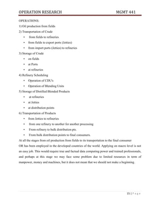
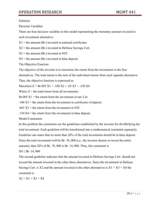
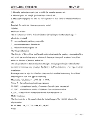
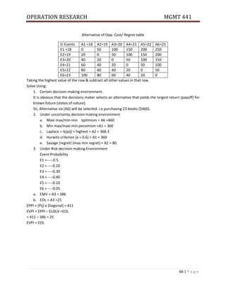
Critical path Analysis
After the project network is drown and activity time is known, we can determine
 The total time needed to complete the whole project.
 When different activities may be scheduled
 Which activities are critical & non-critical?
 The critical path by doing forward and backward pass calculations.
 Float for each activity the amount of time by which the completion of an activity can be
delayed without delaying the total project completion time.
Forward pass calculations give earliest start time (EST) and Earliest finish time (EFT) for each
activity. While backward pass calculations gives latest start time (LST) and latest finish time (LFT)
for each activity.
EFT = EST + Activity duration forward pass calculation
LST = LFT – Activity duration backward pass calculation.
Notation: Activity, Duration [EST, EFT]
[LST, LFT]
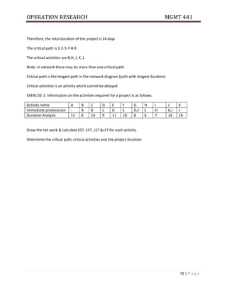
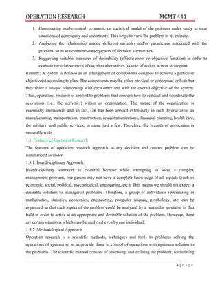
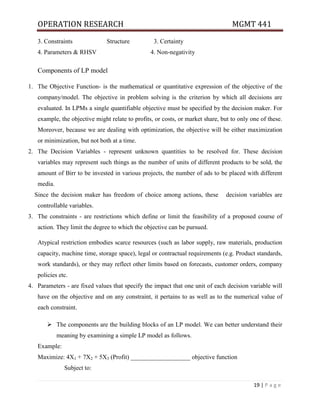
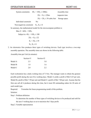
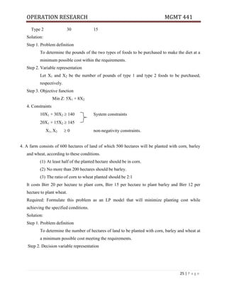
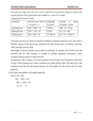
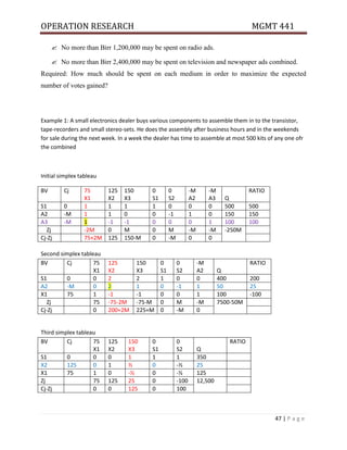
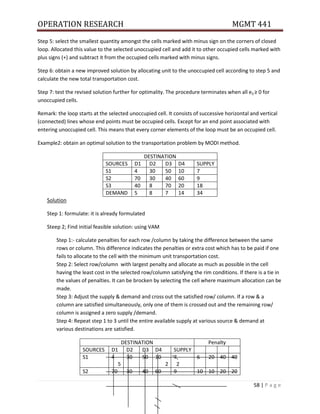
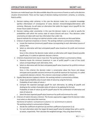
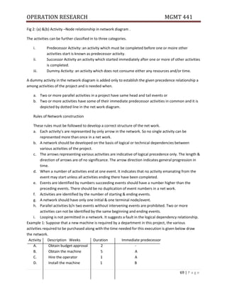
Example 2: Information on the activities required for a project is as follows.
Activity name A B C D E F G H I J K
Activity Node 1-2 1-3 1-4 2-5 3-5 3-6 3-7 4-6 5-7 6-8 7-8
Duration Analysis 2 7 8 3 6 10 4 6 2 5 6
Draw the network & calculate EST, EFT, LST &LFT for each activity.
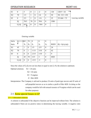
Determine the critical path, critical activities and the project duration
D 3[2,5]
A2[0,2] E6[713] I2[13,15]
B7[0,7] G4[7,11] K6[15,21]
C8[0,8] J5[17,22]
H6[8,14]
1
2
4
3
5
6
7 8

71 | P a g e
Therefore, the total duration of the project is 22 days
The critical path is 1-3-6-8
The critical activities are 1-3, 3-6, 6-8 or B, F and J
Note: in network there may be more than one critical path.
Critical path is the longest path in the network diagram (path with longest duration)
Critical activities is an activity which cannot be delayed
Non critical activity is an activity which can be delayed without affecting the whole project duration.
Float(slack) Sij is the time by which an activity may be delayed without affecting the project duration
Sij= LST-EST/LFT-EFT
Forward pass calculation takes the largest time in merge events in determining EFT
Backward pass calculation takes the least time in burst events in determining LST
Example 2: Information on the activities required for a project is as follows.
Activity name A B C D E F G H I J K L
Immediate predecessor - - - A,B B B C,F B E,H E,H C,D
,F,J
K
Duration Analysis 6 4 10 1 1 3 14 6 9 2 7 5
Draw the net work & calculate EST, EFT, LST &LFT for each activity.
SOLUTION
D K
A J L
B H E I
F
C G
7
1 2 5
9
4
3
8
6

72 | P a g e
Therefore, the total duration of the project is 24 days
The critical path is 1-2-5-7-8-9
The critical activities are B,H, J, K, L
Note: in network there may be more than one critical path.
Critical path is the longest path in the network diagram (path with longest duration)
Critical activities is an activity which cannot be delayed
EXERCISE 1: Information on the activities required for a project is as follows.
Activity name A B C D E F G H I J K
Immediate predecessor - A B C D E D,F E H G,I J
Duration Analysis 13 8 10 9 11 10 8 6 7 14 18
Draw the net work & calculate EST, EFT, LST &LFT for each activity.

OR note.pdf

More Related Content

Similar to OR note.pdf

Recently uploaded

OR note.pdf