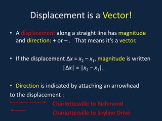
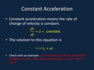
This document provides an overview of one-dimensional motion concepts including: - Distance traveled, displacement, average and instantaneous velocity and acceleration. - Formulas for constant acceleration including relationships between displacement, time, initial velocity, and acceleration. - Examples are provided to illustrate key concepts like the difference between distance and displacement, and calculating average speed from total distance and time.

1. One-Dimensional Motion:
Displacement, Velocity, Acceleration
Physics 1425 Lecture 2
Michael Fowler, UVa.

2. Today’s Topics
• The previous lecture covered measurement,
units, accuracy, significant figures, estimation.
• Today we’ll focus on motion along a straight
line: distance and displacement, average and
instantaneous velocity and acceleration, the
importance of sign.
• We’ll discuss the important constant
acceleration formulas.

3. Kinematics: Describing Motion
Kinematics describes quantitatively
how a body moves through space.
We’ll begin by treating the body as
rigid and non-rotating, so we can
fully describe the motion by
following its center.
Dynamics accounts for the observed
motion in terms of forces, etc. We’ll get to
that later.

4. Measuring Motion: a Frame of Reference
Frame of reference: To measure motion, we must
first measure position.
We measure position relative to
some fixed point O, called
the origin.
We give the ball’s location as
(x, y, z): we reach it from O
by moving x meters along the
x-axis, followed by y parallel
to the y-axis and finally z
parallel to the z-axis.
The frame can be envisioned as
three meter sticks at right angles
to each other, like the beginning of
the frame of a structure.
O
x
y
z
(x, y, z)

5. One-Dimensional Motion: Distance Traveled and
Displacement
• The frame of reference
in one dimension is just
a line!
• Think of a straight road.
• Driving a car, the distance
traveled is what the
odometer reads.
• The displacement is the
difference x2 – x1 from
where you started (x1) to
where you finished (x2).
• They’re only the same if
you only go in one
direction!
O 1
This time we’ve made explicit
that the x-axis also extends in
the negative direction, so we
can label all possible positions.
-1 x

6. Distance and Displacement
• Take I-64 as straight, count Richmond
direction as positive.
• Drive to Richmond: distance = 120 km
(approx), displacement = 120 km.
• Drive to Richmond and half way back:
• Distance = 180 km, displacement = 60 km.
• Drive to closest Skyline Drive entrance:
• Distance = 35 km, displacement = -35 km.

7. Displacement is a Vector!
• A displacement along a straight line has magnitude
and direction: + or – . That means it’s a vector.
• If the displacement Δx = x2 – x1, magnitude is written
|Δx| = |x2 – x1|.
• Direction is indicated by attaching an arrowhead
to the displacement :
Charlottesville to Richmond
Charlottesville to Skyline Drive

8. Average Speed and Average Velocity
• Average speed = distance car driven/time taken.
• Average velocity = displacement/time taken
so average velocity is a vector! It can be negative.
• Formula for average velocity:
• Example: round trip to Richmond.
Average speed = 60 mph ≈ 27 m/sec.
Average velocity = zero!
2 1
2 1
x x x
v
t t t
− ∆
= =
− ∆

9. Instantaneous Velocity
• That’s the velocity at one moment of time: car
speedometer gives instantaneous speed.
• To find this, need to find car’s displacement in a
very short time interval (to minimize speed
variation).
• Mathematically, we write:
This “lim” just means taking a succession of shorter
and shorter time intervals at the moment in time.
0
lim .
t
x dx
v
t dt∆ →
∆
= =
∆

10. Average Trip Speed
You drive 60 miles at 60 mph, then 60 miles at
30 mph. What was your average speed?
A. 40 mph
B. 45 mph
C. 47.5 mph

11. Acceleration
• Average acceleration = velocity change/time taken
• Notice that acceleration relates to change in velocity exactly as velocity relates
to change in displacement.
• Velocity is a vector, so acceleration is a vector.
• Taking displacement towards Richmond as positive:
• Slowing down while driving to Richmond: negative acceleration.
• Speeding up driving to Skyline Drive: also negative acceleration!
2 1
2 1
v v v
a
t t t
− ∆
= =
− ∆

12. Instantaneous Acceleration
• This is just like the definition of instantaneous velocity:
• The instantaneous acceleration
• The acceleration at time t1 is the
slope of the velocity graph v(t)
at that time.
0
lim .
t
v dv
a
t dt∆ →
∆
= =
∆
tt1O
v(t)

13. Our Units for One-Dimensional Motion
• Displacement: meters (can be positive or negative)
• Velocity = rate of change of displacement, units:
Meters per second, written m/s or m.sec-1.
• Acceleration = rate of change of velocity, units:
Meters per second per second, written m/s2 or m.sec-2.

14. Constant Acceleration
• Constant acceleration means the rate of
change of velocity is constant.
• The solution to this equation is
• Check with an example: a car traveling at 10 m/s accelerates
steadily at 2 m/s2. How fast is it going after 2 secs? After 4
secs?
constant.
dv
a
dt
= =
0 .v v at= +

15. Distance Moved at Constant Acceleration
• At constant acceleration,
• The solution of this equation is
• Here x0 is the beginning position, v0 the beginning
velocity, a the constant acceleration.
• Exercise: check this by finding dx/dt.
0( ) .
dx
v t v at
dt
= = +
21
0 0 2( ) .x t x v t at= + +

16. More about Constant Acceleration…
• At constant acceleration,
the graph of velocity as a
function of time v(t) = v0 + at
is a straight line:
• If v = v0 at t = 0, and v = v1 at t = t1, the average velocity over
the time interval 0 to t1 is
• IMPORTANT! This formula is unlikely to be correct at
nonconstant acceleration.
0
v0
v(t)
t1
v1
0 1
.
2
v v
v
+
=

17. Constant Acceleration Formulas
0v v at= +
21
0 0 2x x v t at= + +
0 1
2
v v
v
+
=
( )2 2
0 02v v a x x=+ −
These formulas are worth memorizing: the last one is simply derived
by eliminating t between the first two.

18. The picture below shows time (4.56 secs) and speed
(321 mph) for a standing start quarter mile at
Indianapolis.
Assuming constant acceleration, what was the
approximate horizontal g-force on the driver?
a. 0.3g
b. 0.8g
c. 1.5g
d. 3g
e. 5g