This document summarizes an experiment investigating high-temperature superconductivity in Yttrium Barium Copper Oxide samples. The experiment aimed to demonstrate the Meissner effect and zero resistance in the samples using liquid nitrogen. The document provides theoretical background on superconductivity, including the Meissner effect, Ginzburg-Landau theory, BCS theory, and the structure of Yttrium Barium Copper Oxide. It describes the experimental methods, results from Meissner effect tests, magnetic field experiments, X-ray diffraction analysis, and resistance measurements. The results are then discussed in relation to the theories of superconductivity.

1. Investigation of Superconductivity Theories and the
High-Temperature Superconducting 𝑌𝐵𝑎2 𝐶𝑢3 𝑂7−𝛿
Crystalline Structure
Llyr Humphries – llh18@aber.ac.uk
MPhys - Astrophysics
Institute of Mathematics, Physics and Computer Sciences
Aberystwyth University
3rd Year Project

2. 1
Abstract
The purpose of this set of experiments was to study the nature of high-temperature
superconductivity. Samples of Yttrium Barium Copper Oxide, chosen for its high-
temperature superconductive properties, were used to attempt to demonstrate a zero
resistance system and the phenomenon known as the Meissner effect through the use of
Liquid Nitrogen. This is an important area of research as an analysis of high-temperature
superconductors may lead to the eventual synthesis of room temperature
superconductors; this would entail an enormous leap in technological advancement, with
the potential for ultra-sensitive sensors, energy transfer and faster computers, among
several other possibilities. Yttrium Barium Copper Oxide, particularly 𝑌𝐵𝑎2 𝐶𝑢3 𝑂7−𝛿, was
chosen as the material to be analysed due to its crystalline structure (which is associated
with its superconducting potential) and the large amount of research conducted on the
subject involving this particular compound.
The structure of the Yttrium Barium Copper Oxide samples were researched
through X-Ray diffraction analysis and previously performed experiments to determine
that the perovskite-like, orthorhombic structure of the material (below the critical
temperature) allowed the formation and transfer of Cooper pairs between thin double
layers of Copper Oxide.
Several aspects of superconductivity were researched to gain a better
understanding of the underlying physics of the phenomenon, e.g. Ginzburg-Landau
Theory, BCS Theory, the London equations, and so on. We also attempted to interpret our
observations in terms of these theories (among others), such as abnormally large lattice
parameters and abnormally high critical temperatures relating to Oxygen defects.
Research into the phenomenon known as the quantization of magnetic flux proved
useful in the understanding of theories relating to superconductivity, as a planned
experiment to study this phenomenon involving a superconducting ring was abandoned
due to a lack of appropriate equipment and the non-triviality of such an investigation.

3. 2
Contents
1. Introduction.....................................................................................................................................3
2. Theoretical Aspects........................................................................................................................4
2.1. Introduction to Superconductivity ......................................................................................4
2.2. Meissner effect.........................................................................................................................6
2.3. Ginzburg-Landau Theory......................................................................................................8
2.4. BCS Theory ............................................................................................................................10
2.5. Quantisation of Magnetic Flux..........................................................................................11
2.6. Yttrium Barium Copper Oxide ..........................................................................................13
3. Experimental Method .................................................................................................................15
4. Results ............................................................................................................................................21
5. Discussion ......................................................................................................................................28
5.1 Meissner experiments...........................................................................................................28
5.2 Magnetic field Experiments.................................................................................................28
5.3 XRD...........................................................................................................................................29
5.4 Orthogonal Parameters ........................................................................................................30
5.5 Critical Temperature ............................................................................................................32
5.6 Resistance................................................................................................................................32
5.7 Superconducting ring............................................................................................................34
6. Conclusion......................................................................................................................................35
7. Acknowledgments ........................................................................................................................37
8. References......................................................................................................................................37
9. Literature Review ........................................................................................................................41

4. 3
1. Introduction
While ‘low-temperature’ superconductors and their magnetic and electrical
properties have been studied since the 1910’s, high-temperature superconductivity is a
relatively new field of study. The first high-temperature ceramic superconductor, namely
a Lanthanum Barium Copper Oxide lattice (𝐿𝑎2−𝑥 𝐵𝑎 𝑥 𝐶𝑢𝑂4) with a critical temperature
of 30K [1], was discovered in 1986 by Georg Bednorz and K. Alex Müller, who subsequently
won the 1987 Nobel Prize in Physics. [2]
Superconductivity was first observed by Dutch physicist Heike Kamerlingh Onnes
in 1911 [3] while conducting super-cool experiments on samples of solid Mercury wire. He
observed that the electrical resistivity of the sample abruptly dropped to zero upon cooling
below the sample’s critical temperature, 4.2K (more precisely 4.15K using modern
thermodynamic scales) [4]. Onnes concluded that the sample had passed into a new
superconductive state, so named for its remarkable electrical properties. Onnes was also
unable to provide any form of residual resistance at the lowest temperatures, implying
that a superconductive material possesses zero D.C. electrical resistance. This
phenomenon has startling implications, one of which being the seemingly infinite
persistence of an electrical current within a looped superconducting wire, without
requiring an external power source [1].
This study specifically involves an analysis of only a few aspect of
superconductivity in a high-temperature, type II superconductor, namely an Yttrium
Barium Copper Oxide crystal lattice system (with the general formula 𝑌𝐵𝑎2 𝐶𝑢3 𝑂7−𝑥).
Details of the structure of Yttrium Barium Copper Oxide and the reason for our interest
in this structure will be discussed in chapter 2.6.
The outline of the report is as follows: in chapter 2 the theory concerning
superconductivity will be addressed, beginning with an overview of various concepts of
superconductivity that have been discovered within the last century. After this the
structure of Yttrium Barium Copper Oxide will be discussed, particularly its relationship
with the perovskite structure, and how the previously mentioned theoretical aspects of
superconductivity apply to the samples used in these experiments. Chapter 2 will also
include an analysis of the phenomenon known as the Quantization of Magnetic Flux.
Chapter 3 is concerned with the experimental aspects of this project; the apparatus used
will be included, as well as an explanation and an experimental realization of the sample.
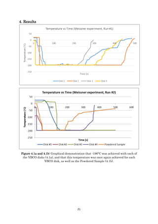
Chapter 4 outlines the results of the experiment; measurement data from the Meissner
and magnetic field experiments will be provided in graphical form, along with graphs
demonstrating the relationship between lattice parameters and critical temperature with
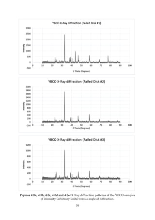
Oxygen defects. X-Ray Diffraction patterns of each sample will also be provided, which
were required in order to determine a possible explanation for several of the disks (as well
as the powdered sample) failing to demonstrate superconductive properties. Chapter 5
will be used to discuss the results outlined in chapter 4, whereby the results of the
Meissner and magnetic field experiments will be analysed to determine if the Meissner
effect had been observed. The X-Ray diffraction patterns of the samples will also be
interpreted with an understanding of High-Tc superconductivity to provide an explanation
for the problem mentioned above. Aspects of the experiment that were not performed will
be discussed, as well as papers that have performed these investigations and how they
would have been implemented for this report. Chapter 6 will simply be used to conclude
the discussion of the results and to provide advice for possible future experiments in this

5. 4
topic and for how to improve on this report’s investigations. Chapter 7 underlines the
acknowledgement of the author for the help received during research on the extremely
wide range of superconductivity background theory and while performing these
experiments.
2. Theoretical Aspects
2.1. Introduction to Superconductivity
Superconductors can be classified in two important ways. The most significant
classification for this report is the division of all superconducting materials by their
critical temperatures, Tc, the temperature at which the material enters the
superconductive state. Superconductors with a critical temperature below 30 Kelvin (K)
belong to the ‘low-temperature’ group, while those with a critical temperature above 30K
fall within the ‘high-temperature’ group.
Another criterion by which to classify superconductors is how the materials
respond to an external, applied magnetic field. If an applied magnetic field exceeds a
critical point (being a ‘critical’ magnetic field unique to every material) it will penetrate
the material, which induces a phase transition from the superconducting state to the
‘normal’ state. Type I superconductors are described by the Pippard theory rather than
the London theory, but the Pippard theory will not be discussed in this report as Yttrium
Barium Copper Oxide is a type II superconductor. Type I superconductors continue to
expel magnetic flux until the applied magnetic field exceeds the critical magnetic field, at
which point the material experiences a sudden phase transition. They usually consist of
pure metals and low concentration alloys. Type II superconductors possess two critical
magnetic fields; 𝐻𝑐1 and 𝐻𝑐2, which allows type II superconductors to occupy one of three
‘regimes’ [5].
If 𝐻 < 𝐻𝑐1 < 𝐻𝑐2 (where 𝐻 is the applied magnetic field) the superconductor is in
its superconducting state and occupies the same regime that a type I superconductor
would occupy when subject to an applied magnetic field below it’s critical value.
If 𝐻 > 𝐻𝑐2 > 𝐻𝑐1 the superconductor is in its normal state and occupies the same
regime that a type I superconductor would occupy when subject to an applied magnetic
field above its critical value.
If 𝐻𝑐2 > 𝐻 > 𝐻𝑐1 the superconductor is in what is commonly called the ‘mixed state’
or ‘vortex state’, in which the applied magnetic field partially penetrates the
superconductor. The parts of the superconductor which have been penetrated by the
magnetic field will be in their normal state with currents circulating around them. Type
I and II superconductors also have critical temperatures (which shall be discussed
shortly), which the critical fields of both type of superconductors are a function of.
Below, figure 2.1.1 shows a schematic variation of the magnetisation versus
critical magnetic field strength for type I and II superconductors, and in figure 2.1.2 shows
a characteristic phase diagram for type I and II superconductors.

6. 5
Figure 2.1.1 [6]: Schematic variation of induced magnetic field versus an applied
magnetic field. An induced magnetic field of zero implies that the material is no longer
superconducting.
The larger dotted triangle in figure 2.1.1 represents the abrupt switch of states
experienced by a type I superconductor as it transitions from the superconducting state
to the normal state (as its critical field is exceeded). The smaller triangle represents the
transition of a type II superconductor from the superconducting state to the mixed state
as 𝐻𝑐1 is exceeded, with a more gradual transition to the normal state as the applied
magnetic field penetrates more of the material.
Figure 2.1.2 [7]: Phase diagram for type I and type II superconductors. The phase
diagram for a type II superconductor is shown as a solid line.
In figure 2.1.2, while a type II superconductor lies below the 𝐻𝑐1 curve (curved due to the
critical magnetic field’s dependence on the temperature of the material), the
superconductor is in its superconducting state. However, if the superconductor lies above
the 𝐻𝑐2 curve (also curved due to the reason stated above) the superconductor is in its

7. 6
normal state. Between 𝐻𝑐1 and 𝐻𝑐2 a type II superconducting material is said to be in its
mixed state. Above the dashed 𝐻𝑐 curve, a type I of superconductor is said to be in its
normal state. Alternatively if the material is below the 𝐻𝑐 curve it is said to be in its
superconducting state.
For the purpose of this report, a type II, high-temperature superconductor was
studied in our experiments. Although other variations of superconductors were not used,
it was still useful to research how to distinguish between them and their individual
properties.
2.2. Meissner effect
The Meissner effect (shortened from the Meissner-Ochsenfeld effect) was observed
by Walther Meissner and Robert Ochsenfeld in 1933 during an experiment intended to
demonstrate that superconductors were merely perfect conductors through the use of
classical electromagnetism [8]. In light of experiments performed by Onnes and Tuyn and
by applying Maxwell’s equations, Meissner and Ochsenfeld attempted to demonstrate
that the infinite conductivity of a material implies that bringing about any change of
magnetic field within the material is impossible, which also implies that flux within the
superconductor would become ‘frozen in’ at the instant of transition [9]. Contrary to their
predictions, superconductors behaved differently to a theoretically perfect conductor.
Their experiment involved subjecting a Lead sample to a weak magnetic field above its
critical temperature, and then reduced its temperature below 7.22 K [10], expecting
magnetic flux to have been trapped within the sample. This would have meant that a
subsequent removal of the applied magnetic field would have left the sample with internal
magnetic flux. However, it was observed that the internal magnetic flux was expelled,
giving an effective permeability of -1 (perfect diamagnetism) [11]. The magnetic field
strength immediately outside the lead sample increased, while the normal component of
the field appeared to be zero, indicating an expulsion of the internal magnetic field and a
perfect diamagnetic state. An interesting characteristic of the expulsion of flux is that the
phenomenon would occur whether a superconducting material was first placed in a
magnetic field and then cooled below the critical temperature or vice versa [8]; this was
particularly useful for our experiment, as it was difficult to place the rare-Earth magnet
above the sample before the sample was cooled.
If a superconductor in the normal state is subjected to an applied magnetic field
and then cooled below its critical temperature (or vice versa) an electric current rapidly
builds up on the superconductor’s surface, producing a magnetic field that suppresses the
magnetic flux within the interior, thus allowing the levitation of a magnet above the
superconductor [12]. Below is an illustration of the Meissner effect and how surface
currents are induced.

8. 7
Figure 2.2.1: [13] Image demonstrating the Meissner effect. (a) shows a
superconductor above its critical temperature (left), allowing magnetic flux to enter the
material, alongside an image of a superconductor below its critical temperature (right)
causing surface currents (represented by the red arrow) to circulate around the sample,
inducing a magnetic field which cancels the applied magnetic field. (b) demonstrates the
induced surface current loop levitating a magnet above a superconductor’s surface.
In fact, the applied magnetic field does penetrate the surface of the superconductor
to some extent within a thin layer, known as the penetration depth, which may be derived
from the London equations.
Developed by Fritz and Heinz London in 1935, the London equations explains the
Meissner effect. The equations describe the exponential expulsion of all internal magnetic
fields from a superconducting material as it transitions to the Meissner state (for clarity
the ‘Meissner state’ and the ‘Superconducting state’ are synonymous). There are several
ways to justify the London equations, but perhaps the most acute is the quantum method
involving the vector potential A, given by Fritz London [14]. Noting that the
superconducting current density is defined as
𝒋 𝒔 = 𝑛 𝑠 𝑒𝒗 (2.2.1)
where 𝑛 𝑠 is loosely associated with the number density of superconducting carriers, e is
the electronic charge and 𝒗 is the velocity of the charge carriers. The canonical
momentum is defined as
𝒑 = 𝑚𝒗 + 𝑒𝑨/𝑐 (2.2.2)
where m is the electron mass and c is the speed of light. The ‘single’ London equation can
be described by using Bloch’s theorem to argue that the canonical momentum in a
system’s ground state is zero, and by combining equations 2.2.1 and 2.2.2 it can be shown
that
𝒋 𝒔 = −
𝑛 𝑠 𝑒2
𝑨
𝑚𝑐
(2.2.3)
Taking the time derivative of both sides of equation 2.2.3 yields the first of the London
equations;
𝜕𝒋 𝒔
𝜕𝑡
=
𝑛 𝑠 𝑒2
𝑚
𝑬
(2.2.4)

9. 8
where E is the electric field. Taking the curl of both sides of 2.2.3 leads to the second
London equation;
∇ × 𝒋 𝒔 = −
𝑛 𝑠 𝑒2
𝑚
𝑩
(2.2.5)
where B is the magnetic field. By applying Ampere’s Law to 2.2.5 it can be manipulated
[14] to produce the following equation;
∇2
𝑩 =
1
𝜆2
𝑩
(2.2.6)
where
𝜆 ≡ √
𝑚𝑐2
4𝜋𝑛 𝑠 𝑒2
whereby 𝜆 is the London penetration depth, implying a characteristic length scale at
which an applied magnetic field becomes exponentially weaker than the magnetic field at
the surface of the superconductor [15].
2.3. Ginzburg-Landau Theory
The Ginzburg-Landau (GL) Theory was initially postulated as a macroscopic model
to describe type I superconductors without examining their microscopic properties in
great detail. However, a version of the GL theory was later derived from the Bardeen-
Cooper-Schrieffer theory by L. P. Gor’kov, demonstrating that it can be interpreted
microscopically, e.g. the order parameter of the GL theory is related to the wave function
of Cooper pairs [16].
Developed by V. L. Ginzburg and L. Landau in the 1950’s, they proposed the
introduction of a quantity, Ψ, known as the order parameter, which is defined as equal to
zero for a normal region and unity for a fully superconducting region at T = 0 [17]. Ψ was
taken to be a complex quantity, the modulus squared of which was equal to the number
density of superconducting charge carriers, such that
|Ψ(𝑟)|2
= 𝑛 𝑠(𝑟)
Based on a theory established by Landau on second-order phase transitions, the
free energy of a superconducting system near transition can be expressed as a power
series in |Ψ|2
, the coefficients of which are functions of temperature [18], such that
𝐹 = 𝐹𝑛 + 𝛼|Ψ|2
+
𝛽
2
|Ψ|4
+
1
2𝑚
|(−𝑖ℏ∇ − 2𝑒𝑨)Ψ|2
+
|𝑩|2
2𝜇0
(2.3.1)
where 𝐹𝑛, e and m are the free energy of the normal state in which Ψ = 0, the effective
mass and the electron charge, respectively, A is the magnetic vector potential, B is the
magnetic field such that 𝑩 = ∇ × 𝑨, and 𝛼 and 𝛽 are phenomenological parameters. By
minimizing the free energy with respect to Ψ and A, one arrives at the two GL equations;
𝛼Ψ + 𝛽|Ψ|2
Ψ +
1
2𝑚
|(−𝑖ℏ∇ − 2𝑒𝑨)|2
Ψ = 0
(2.3.2)

10. 9
𝒋 =
2𝑒
𝑚
(Ψ∗(−𝑖ℏ∇ − 2𝑒𝑨)Ψ)
(2.3.3)
where j is the current density which is equal to the superconducting current density while
the material is in the superconducting state [19]. It is worth mentioning that the 2𝑒 within
the modulus of equation 2.3.2, the first GL equation, was previously denoted 𝑒∗
, being the
effective charge of the superelectron wavefunction. The denotation was later changed to
account for Cooper Pairs [20] (which will be discussed in section 2.4). The physics behind
the derivation of the two GL equations is rather complicated and therefore will not be
discussed in full in this report.
The second GL equation may be re-written as
𝒋 𝒔 = −
2𝑒ℏ𝑛 𝑠
𝑚
(∇𝜃 +
2𝑒𝑨
ℏ
)
(2.3.4)
by setting
Ψ = 𝑛 𝑠
1
2
𝑒 𝑖𝜃
|Ψ|2
= 𝑛 𝑠 = −
𝛼
𝛽
which follows from the London approximations of a homogeneous superconductor below
𝑇𝑐
[19] [21] [24], whereby
𝛼(𝑇) = (
𝑑𝛼
𝑑𝑇
)
𝑇𝑐
(𝑇 − 𝑇𝑐) for 𝑇 ≤ 𝑇𝑐
𝑑𝛼
𝑑𝑇
> 0 for 𝑇 = 𝑇𝑐
𝛽 = 𝛽(𝑇𝑐) ≡ 𝛽𝑐 > 0
By then taking the curl of equation 2.3.4 (the second GL equation), while considering that
∇ × ∇𝜃 = 0 and ∇ × 𝑨 = 𝑩, one arrives at
∇ × 𝒋 𝒔 = −
4𝑒2
𝑛 𝑠
𝑚
𝑩 (2.3.5)
Also worth considering is
𝜇0∇ × 𝒋 𝒔 = ∇ × (∇ × 𝑩) = −∇2
𝑩
Thus equation 2.3.5 can we rewritten as

11. 10
∇2
𝑩 =
𝑩
𝜆2
where
𝜆 = √
𝑚
4𝜇0 𝑒2 𝑛 𝑠
= √
𝑚
4𝜇0 𝑒2|Ψ|2
which demonstrates that the second GL equation is in accordance with the second London
equation under certain conditions, meaning that the GL theory can predict the Meissner
effect and that the London equations are consequences of the coherence of a quantum
state [23].
Equation 2.3.2 is a non-linear form of the free-particle Schrödinger equation and
can be rearranged to
𝜉2
∇2
Ψ + Ψ −
𝛽
|𝛼|
|Ψ|2
Ψ = 0
Where
𝜉 = √
ℏ2
2𝑚|𝛼|
(2.3.6)
whereby 𝜉 is the coherence length and is defined as the parameter by which |Ψ| varies
due to small perturbations in superconducting electron density. Equation 2.3.6 is valid
only for superconductors in the normal state. The coherence length of superconductors in
the Meissner state can be defined as
𝜉 = √
ℏ2
4𝑚|𝛼|
Whereby 𝑚 in equation 2.3.6 is replaced by 2𝑚 due to the formation of Cooper pairs in the
Meissner state. A new parameter can be defined from the coherence length and
penetration depth of the material known as the Ginzburg-Landau parameter;
𝜅(𝑇) =
𝜆(𝑇)
𝜉(𝑇)
and remains finite as 𝑇 → 𝑇𝑐. Type I superconductors are defined by 𝜅 < 1/√2 and type II
superconductors are defined by 𝜅 > 1/√2 [24].
2.4. BCS Theory
To begin, it is worth mentioning the importance of H. Fröhlich’s model of electron-
phonon interactions. While the model was specified for metals, it is applicable to other
materials. The model describes continuous phononic interactions of an electron with its
surrounding lattice, causing perturbations in its neighbouring atoms, to which the
electron reacts [25]. Fröhlich argued that this interaction could produce a ground state of
lower energy electrons relative to the Fermi level of non-interacting electrons, and that
this Superconducting ground state would be separated from normal conducting states by
an energy gap (the Fermi level) [26]. Although ‘gapless’ superconductors exist, they will not

12. 11
be discussed in this report. The phonon-electron interaction model was supported by two
experimental investigations in the 1950’s on the variation of 𝑇𝑐 as 𝑀−1/2
, where M is the
isotopic mass [27] [28], which is a result of the model if phonon-electron interactions are
important.
L. N. Cooper was the first to propose an electron-phonon-electron interaction which
could result in a reduction of the Coulomb repulsion between two electrons in the
superconducting state, relative to the normal state [29]. Cooper suggested the following
sequence of events: an electron induces the creation of a phonon as it deforms the
surrounding lattice by attracting positive charges; the phonon then propagates through
the lattice and is subsequently absorbed by another electron with opposite spin; the
second electron then moves into a region of higher positive charge density. Since the
phonon exchange is virtual, energy is conserved in the lattice, but not between the two
electrons. With this suggestion, Cooper showed that if the phonon exchange resulted from
an attractive interaction (regardless of origin), a bound state of an electron pair could
result [30].
Bardeen, Cooper and Schrieffer then followed this suggestion by showing that
bound pairs of electrons of opposing spin and exactly opposite values of wave vector, could
form under favourable conditions [31] [32]. The existence of these ‘Cooper pairs’ is strongly
implied by evidence from flux quantisation experiments, which will be discussed in section
2.5.
While Cooper pairs are symmetric about 𝒌 = 0 for a superconductor with zero
current density, where k is the wave-vector in a non-vanishing persistent current
situation, the Fermi sphere is shifted bodily. This results in all Cooper pairs gaining a
non-zero momentum. The current carried by these Cooper pairs cannot be relaxed by
phonon activity or local defects due to the energy gap stabilising them from small net
changes of momentum; the breaking of a single pair would change the energy of the entire
‘condensed’ state of pairs, thus the energy required to break a single Cooper pair is related
to the energy required to break all Cooper pairs. This gives rise to the infinite (D.C.)
conductivity of superconductors as an essential consequence of BCS theory [25]. The BCS
theory also implies the Meissner effect, but to demonstrate this is beyond the level of this
report.
2.5. Quantisation of Magnetic Flux
F. London predicted the quantisation of magnetic flux trapped within a
superconducting ring in the 1950’s, implying that a quantum mechanical effect is
observable on the macroscopic scale [33] [34]. Flux quantization has been observed in type I
and type II superconductors, primarily in situations involving a superconducting material
surrounding a non-superconducting hole (e.g. a hollow superconducting cylinder,
superconducting ring or a superconducting toroid. A superconducting material subjected
to an applied magnetic field is cooled below its critical temperature, causing magnetic flux
to be ejected from the material. However, the magnetic flux will not be ejected from the
inner non-superconducting region. A subsequent removal of the applied magnetic field
would result in the trapping of the flux lines within this region and are maintained by
persistent currents in the surrounding superconducting material [15].
London also predicted the quantized units of the trapped magnetic flux as

13. 12
Φ 𝑜 =
2𝜋ℏ
𝑒
= 4.14 × 10−15
𝑊𝑏
based on the suggestion that the trapped magnetic flux should be quantized since
superconductivity is overtly a quantum phenomenon [35].
The method of deriving the flux quantum value discussed in this report involves
employing the time-dependent Schrödinger equation to derive the second GL equation
and integrating around a closed loop. The Cooper pair condensate can be described as a
single macroscopic wave function
Ψ(𝒓, 𝑡) = |Ψ(𝒓, 𝑡)|𝑒 𝑖𝜃(𝒓,𝑡) (2.5.1)
where Ψ(𝒓, 𝑡) is the quantum mechanical wave function, |Ψ(𝒓, 𝑡)| is the amplitude of the
wave function and 𝜃(𝒓, 𝑡) is the phase at position r and time t [36]. Equation 2.5.1 must
obey the time-dependent Schrödinger equation [37]
[
1
2𝑚
(
ℎ
𝑖
∇ − 𝑞𝑨)
2
+ 𝑞Φ] Ψ = 𝑖ℏ
𝜕Ψ
𝜕𝑡 (2.5.2)
Where m and q are the mass and charge of the Cooper pairs, respectively and Φ(𝒓, 𝑡) is
the scalar potential. By multiplying equation 2.5.2 by Ψ∗
and by subtracting its complex
conjugate, one finds
−∇ ∙ [
ℏ
2𝑚𝑖
(Ψ∗
∇Ψ − Ψ∇Ψ∗) −
𝑞
𝑚
|Ψ|2
𝑨] =
𝜕
𝜕𝑡
(Ψ∗
Ψ)
(2.5.3)
and by multiplying equation 2.5.3 by q one obtains the equation of electromagnetic
continuity
−∇ ∙ 𝒋 𝒔 =
𝜕𝜌𝑠
𝜕𝑡
where 𝜌𝑠 is the charge density and
𝒋 𝒔 =
ℏ𝑞
2𝑚𝑖
(Ψ∗
∇Ψ − Ψ∇Ψ∗) −
𝑞2
𝑚
|Ψ|2
𝑨
(2.5.4)
Which may be rearranged to produce equation 2.3.3. By substituting equation 2.5.1 into
2.5.4 and by assuming that Ψ∗
Ψ can be interpreted as the local charge carrier density, 𝑛 𝑠,
one arrives at
𝒋 𝒔 =
ℏ𝑞𝑛 𝑠
𝑚
(∇𝜃) −
𝑞2
𝑛 𝑠
𝑚
𝑨 (2.5.5)
By integrating equation 2.5.5 around a closed loop Γ [33] [38] [39], one obtains
∮ 𝒋 𝒔
Γ
. 𝑑𝒍 = ∮
ℏ𝑞𝑛 𝑠
𝑚Γ
(∇𝜃). 𝑑𝒍 − ∮
𝑞2
𝑛 𝑠
𝑚Γ
𝑨. 𝑑𝒍 (2.5.6)
By invoking Stokes’ Theorem

14. 13
∮ 𝑨
Γ
. 𝑑𝒍 = ∮(∇ × 𝑨)
s
. 𝑑𝑺 = ∮ 𝑩
s
. 𝑑𝑺 = Φ
by recognising that equation 2.5.1 must be single valued and that integrating ∇𝜃 around
a closed loop yields 2𝜋𝑥 (𝑥 ∈ ℝ), and by also assuming that the path of integration is a line
where 𝒋 𝒔 = 0 [39], equation 2.5.6 may be rearranged to predict flux quantization [40];
ℏ𝑞𝑛 𝑠
𝑚
(2𝜋𝑥) =
𝑞2
𝑛 𝑠
𝑚
Φ
⇒ ℏ(2𝜋𝑥) = 𝑞Φ
⇒ Φ =
ℎ
𝑞
𝑥 = 𝑥Φ0
in which
Φ0 ≡
ℎ
|𝑞|
=
ℎ
2𝑒
= 2.07 × 10−15
𝑊𝑏
(2.5.7)
Which is half the value predicted by London.
Equation 2.5.7 (with the implication of −2𝑒 as the fundamental superconducting charge)
agrees with the Cooper pair concept of BCS theory and the suggestion that charge carriers
in a superconductor in the Meissner state are pairs of electrons of opposite spin and wave
vector. This has been verified in various experiments whereby magnetic flux has been
isolated [41] [42].
2.6. Yttrium Barium Copper Oxide
It would be useful to begin this section by discussing the perovskite structure. A
compound with a crystalline structure similar to that of Calcium Titanium Oxide is said
to possess a perovskite structure. Perovskite compounds typically have the chemical
formula of 𝐴𝐵𝑋3 where A and B are different species of cation (whereby A is drastically
larger than B) and X is an anion (typically a species of Halogen) that bonds with both
cation species [43]. The ideal perovskite structure is a cubic unit cell consisting of a primary
cation (A) at the centre of the unit cell, another cation (B) at each corner of the unit cell,
and an octahedron of anions at the face-centred positions [44]. The relative ion sizes
required for the stability of the cubic lattice are precise, therefore deviation (e.g. anion
octahedral tilt or distortion, cation displacement etc.) [45] from these requirements may
result in lower-symmetry distortions of the perovskite structure. The most common
perovskite distortions are the orthorhombic and tetragonal non-cubic variants. The
orthorhombic variant results from the cubic lattice stretching along two of its orthogonal
pairs by different factors, resulting in a rectangular prism with a rectangular base (such
that 𝑎 ≠ 𝑏 ≠ 𝑐). The tetragonal lattice results from the cubic lattice stretching along one
of the lattice vectors, resulting in a rectangular prism with a square base (such that 𝑎 =
𝑏 ≠ 𝑐 where c is the height of the lattice). Certain complex perovskite structures contain
two different B-site cations, one of which is Yttrium Barium Copper Oxide. This property
can result in ordered and disordered variants, which can result in dramatically different
electrical properties, which will be discussed shortly.

15. 14
Figure 2.6.1: Image of the ideal perovskite structure, shown as bonded atoms (left)
and as conrner-linked octahedra (right) [44] The primary cation, secondary cations and
anions are denoted by the red, blue and green circles, respectively.
Yttrium Barium Copper Oxide (YBCO) is a crystalline compound consisting of an
orthorhombic lattice structure (with the following ideal orthogonal parameters; 𝑎 =
3.823 Å, 𝑏 = 3.885 Å, 𝑐 = 11.7 Å) [50], resulting from a defective perovskite structure [46].
The YBCO unit cell consists of a layer of CuO, a layer of BaO surrounded by four Oxygen
ions, a layer of 𝐶𝑢𝑂2 surrounded by 5 Oxygen ions in a polyhedral shape, and a layer of
Oxygen-deficient Yttrium. Below is an illustration of the structure of YBCO.
Figure 2.6.2: Image of the YBCO structure, consisting of a perovskite-like
structure with an orthorhombic lattice system whereby 𝑎 ≠ 𝑏 ≠ 𝑐 with all three
orthogonal bases intersecting at 900 [47].
The 𝐶𝑢𝑂2 planes along the b-axis directly above and below the Yttrium atom have
two Oxygen atoms per Copper atom, which compared to the ideal perovskite structure
(where four Oxygen atoms would be present) are said to be Oxygen deficient; these Copper
Oxide layers are believed to be essential to superconductivity, as they are common to the
Cuprate Superconductors [48] [49].
YBCO can be regarded as a derivative of 𝑌𝐵𝑎2 𝐶𝑢3 𝑂6 by oxidation, providing additional
𝑂2−
charge carriers. However, this process does not saturate the structure with additional
Oxygen, resulting in a number of vacancies in the lattice. The general chemical formula
of YBCO is therefore usually written as 𝑌𝐵𝑎2 𝐶𝑢3 𝑂7−𝛿, where – 𝛿 represents the Oxygen
defects in the structure. If 𝛿 > 0.65 the YBCO structure is tetragonal (due to the vacancies

16. 15
in the Oxygen sites in the CuO layers), which is a form of YBCO which is insulating,
rather than superconducting [50] [51].
Figure 2.6.3: Image comparing the orthorhombic structure of 𝑌𝐵𝑎2 𝐶𝑢3 𝑂7 (left)
with the tetragonal structure of 𝑌𝐵𝑎2 𝐶𝑢3 𝑂6 (right) [50]
Superconductivity occurs in 𝑌𝐵𝑎2 𝐶𝑢3 𝑂7−𝛿 when 0 < 𝛿 < 0.65. As the dopant (Oxygen
content) increases from 𝛿 = 1, the hole concentration of the charge reservoir (CuO layers)
increases until a ‘threshold value’ is achieved (at 𝛿 ≈ 0.65), at which point positive charge
spills over to the 𝐶𝑢𝑂2 planes, which results in superconducting 𝐶𝑢𝑂2 planes [52]. The
current flows through these planes because the distance between the Copper atoms is
preferable to the distance between the Copper Oxide planes. A natural consequence of
this is that the current flow is dependent upon the crystal orientation, and performs best
when the current flows parallel to the 𝐶𝑢𝑂2 plane.
The occurrence of superconductivity in the YBCO structure is not well understood,
since no predictive theory is currently known. The evaluation of the superconducting
measurements is complicated (due to ambiguous reasons for superconductivity) [53]
although a range of theories have been put forward. Examples of these theories include
the application of the strong and weak coupling theories [54]. Also, more intensely
researched, is an adaptation of the phonon-based BCS-Eliashberg theory [55] [56] [57], in
which the original BCS theory is extended to include dynamic phonon exchange with
electron-phonon interactions as the principle cause for attractive interaction between
electrons [58]. However, Eliashberg and others haven’t considered this theory particularly
useful for discovering new High-Tc superconductors, as the theory doesn’t accurately
predict the normal state of superconductors. Interestingly, Bednorz and Müller (among
others) developed concepts describing strong electron-phonon coupling in metallic oxides
from various ideas, including the BCS theory [59] [60].
3. Experimental Method
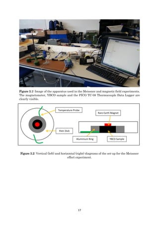
The experimental side of the report comprised of three main objectives: observing
the Meissner effect in any of the YBCO samples; providing measurable evidence of
superconductivity e.g. readings of magnetic field variation around the samples and zero

17. 16
electrical resistance through the samples; and to perform X-Ray Diffraction on working
and failed samples to determine the cause of superconductivity and lack-of, respectively.
The original intent was to synthesise samples of YBCO by using sol-gel techniques,
a process which involves the production of solid material samples (primarily the
fabrication of metal oxides), whereby monomers are converted into a colloidal solution (or
‘sol’) which is a precursor for an integrated network (or ‘gel’) of polymers or discrete
particles. This method would have involved the development of a powdered YBCO sample
through a sequence of processes from a colloid to a gel-like system, drying and
densification, and a firing process in an enclosed furnace tube with an Oxygen
atmosphere. The Oxygen atmosphere would have been necessary in order to sinter the
sample to a preferred crystalline structure (whereby the sample could be appropriately
doped with Oxygen). While this technique of synthesising YBCO samples would have been
relatively straightforward, the annealing process required to manipulate the defects and
orthogonal parameters of the crystalline structure would be somewhat more complicated.
Instead, it was decided (as well as advised) that four 14 mm diameter, pre-prepared YBCO
disk-shaped samples should be purchased for the experiment. This decision was made
after considering the time required to design and develop an annealing furnace and
annealing programme, as well as the prospect of the synthesised YBCO samples failing
to demonstrate any signs of superconductive attributes.
The first goal was to determine whether or not the YBCO samples were
superconducting. Each sample was placed within an Aluminium ring (which had been
designed so that the disks would fit within the inner circle). The aluminium/YBCO system
was subsequently placed within a glass petri dish upon a slab of wood (acting as an
insulated surface). A four temperature-probe system was used; one temperature probe
was placed in a pin hole within the aluminium ring, another was placed outside the
aluminium ring (but still within the petri dish), while the remaining two probes were used
as controls (measuring room temperature). The temperature probes were connected to a
PICO TC-08 Thermocouple Data Logger, further connected to a computer with an
appropriate program for displaying measurements of temperature. Liquid Nitrogen was
then used to cool the disks to below their critical temperature. Liquid Nitrogen was an
appropriate cooling agent because the highest recorded critical temperature of YBCO is
approximately 92 K, whereas the boiling point of Liquid Nitrogen is approximately 77 K.
Once the samples were below their critical temperature, a rare-Earth magnet was placed
slightly above the YBCO samples to determine if they would levitate and thus
demonstrate the Meissner effect. The temperature readings from the samples would be
recorded regardless of the outcome as evidence that the samples reached their critical
temperature. Below is an image of the apparatus used in the experiment, as well as a
diagram of the experimental set-up for the first part of the experiment.

18. 17
Figure 3.1: Image of the apparatus used in the Meissner and magnetic field experiments.
The magnetometer, YBCO sample and the PICO TC-08 Thermocouple Data Logger are
clearly visible.
Figure 3.2: Vertical (left) and horizontal (right) diagrams of the set-up for the Meissner
effect experiment.
YBCO SampleAluminium Ring
Temperature Probe
Petri Dish
Rare-Earth Magnet

19. 18
Figure 3.3a and 3.3b: powdered YBCO sample encased in aluminium foil (left) and solid
YBCO sample (right), each with a rare-Earth magnet placed above.
None of the YBCO disks demonstrated superconductive phenomenon, so it was
decided that a ‘guaranteed’ superconducting sample should be obtained from elsewhere.
A powdered YBCO sample was obtained, and the experiment performed on the solid disks
was repeated with the powdered sample, but with a thinner, wider rare-Earth magnet –
the powder was pressed into the inner circle of the aluminium ring which was surrounded
by two layers of aluminium foil to prevent liquid Nitrogen from disturbing the powder.
The powdered sample also failed to demonstrate the Meissner effect. The
temperature of the sample was recorded throughout the experiment, as explained above.
For this reason it was decided to repeat the initial experiment with the solid YBCO disks,
but now with the thinner magnet. Upon testing the four disks, one successfully displayed
the Meissner effect by levitating the rare-Earth magnet in place above itself.
With a working superconducting sample, the next part of the experiment was
performed, namely the magnetic field measurement. The apparatus was re-arranged so
that the rare-Earth magnet would be situated beneath the petri dish. An additional quad-
temperature probe was also attached to the apparatus as a secondary means of measuring
temperature. A magnetometer/GLX Xplorer system was set up, with the magnetometer
situated closely above the YBCO disk to measure the magnetic field immediately outside
the YBCO disk. The magnetic field was continuously measured as the liquid Nitrogen was
applied and as the YBCO sample reached its critical temperature. This was then repeated
without the YBCO sample, whereby the petri dish and the rare-Earth magnet would be
cooled to approximately 77 K. The differences between these results will be discussed in
chapter 5.

20. 19
Figure 3.4: Vertical, from below (left) and horizontal (right) diagrams of the set-up of the
magnetic field experiment.
Figure 3.5: Image of the magnetic field set-up, where the magnetometer is positioned
above the YBCO/aluminium ring system.
An attempt to measure the resistance across the working YBCO disk was made
using silver epoxy as a ‘resistance free’ substance for providing Ohmic contact between
the copper wires (connected to a multimeter) and the superconductor. This part of the
experiment was abandoned due to complications, which will be discussed in chapter 5.
Although several of the YBCO samples failed to demonstrate any superconductive
properties, this granted an opportunity to analyse the crystalline structure of a working
sample together with a failed sample so that the differences in crystalline structure (if
any) between the samples may be considered to determine why superconductivity arose
in only one of the samples. This lead to the third part of the experiment; performing X-
Ray Diffraction on the working and failed YBCO samples.
Rare-Earth MagnetAluminium Ring
Temperature Probe
Petri Dish
Magnetometer YBCO sample

21. 20
Figure 3.6: Image of the X-Ray Diffractometer performing XRD on the working YBCO
sample (situated on the small platform at the centre of the image).
X-Ray diffraction involves the scattering of incident X-Rays (from the left arm of the
diffractometer above) by electrons in the regular atomic arrays of a crystalline structure.
This scattering produces secondary spherical waves emanating from the electrons; a
phenomenon known as elastic scattering. A regular atomic array produces a regular array
of spherical waves, most of which cancel each other out; a phenomenon known as
destructive interference. If the diffraction angle of the initial X-Rays are appropriate, the
spherical waves will interact constructively. This constructive interference is detected by
the right arm of the diffractometer and interpreted as a peak in the diffraction pattern,
demonstrating the structure of the lattice.
The diffractometer performed 16 runs for each sample to increase the accuracy of
the diffraction patterns. The background X-Ray radiation and the 𝐾𝛼2 background
readings were subtracted from the initial results. The orthogonal lattice parameters of
the samples were also determined via X-Ray diffraction, as well as the crystal system,
Hermann-Mauguin Notation, crystal class and chemical formulae, which were
subsequently compared with literature values
The powdered sample was intended to be used in a superconducting ring system
in order to study the quantization of magnetic flux. This would have achieved by
measuring minute changes in the induced magnetic field of the ring (through the use of a
SQUID) by increasing the applied magnetic field (while the superconducting ring was
below its critical temperature). Due to the non-triviality of this part of this experiment,
and the fact that the appropriate equipment wasn’t available, it was decided that this
part of the experiment would not be performed, but that the phenomenon was still worth
studying. This will be discussed further in chapter 5.

22. 21
4. Results
Figure 4.1a and 4.1b: Graphical demonstration that -196°C was achieved with each of
the YBCO disks (4.1a), and that this temperature was once again achieved for each
YBCO disk, as well as the Powdered Sample (4.1b).

23. 22
Figures 4.2a and 4.2b: Images of the rare-Earth magnet levitating above the YBCO
sample.
-50
-40
-30
-20
-10
0
10
20
30
0 200 400 600 800 1000 1200
ManeticField(mT),Temperature(°C/10)
Time (s)
Magnetic Field and Temperature vs Time (run #1)
Axial H Field Perpendicular H Field Temperature Quad Temperature Pico
-40
-30
-20
-10
0
10
20
30
0 200 400 600 800 1000 1200
MagneticField(mT),Temperature(°C/10)
Time (s)
Magnetic Field and Temperature vs Time (Run #2)
Axial H Field Perpendicular H Field Temperature Quad Temperature Pico

24. 23
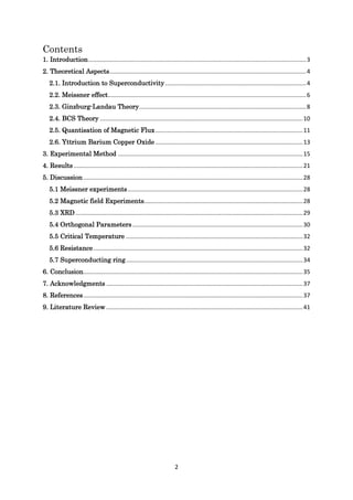
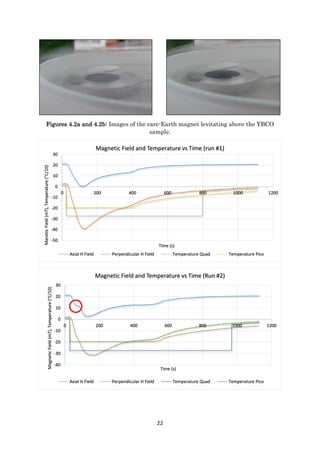
Figures 4.3a, 4.3b and 4.3c: Graphical representation of magnetic field immediately
outside the YBCO sample) and temperature measurements vs time. Figure 4.3c
represents the experiment run without the YBCO disk present. The red circle in figure
4.3b will be discussed in chapter 5.
Figure 4.4: Graph demonstrating the dependence of the critical temperature of
𝑌𝐵𝑎2 𝐶𝑢3 𝑂7−𝛿 on the oxygen defect 𝛿 [50].
Figures 4.5a and 4.5b: Graphs of orthogonal parameter lengths vs oxygen defects (and
stoichiometry) [61].
-40
-30
-20
-10
0
10
20
30
0 200 400 600 800 1000 1200
MangneticField(mT),Temperature(°C/10)
Time (s)
Manetic Field and Temperature vs Time (without disk)
Axial H Field Temperature Quad Temperature Pico Perpendicular H Field

25. 24
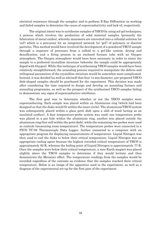
Figure 4.6: Graph demonstrating the dependence of the structure of 𝑌𝐵𝑎2 𝐶𝑢3 𝑂7−𝛿 on the
occupancy of the O1 and O5 sites (located in the a – and b – axes, respectively) and the
oxygen deficiency [39].
Figure 4.7a: Literature XRD pattern of 𝑌𝐵𝑎2 𝐶𝑢3 𝑂7 from 20° to 60° [62].

26. 25
Figure 4.7b: XRD pattern of 𝑌𝐵𝑎2 𝐶𝑢3 𝑂7−𝛿 from 10° to 90° (annealed in 𝑂2 at 1153 K)
obtained from a paper on YBCO synthesis techniques [63].

27. 26
Figures 4.8a, 4.8b, 4.8c, 4.8d and 4.8e: X-Ray diffraction patterns of the YBCO samples
of intensity (arbitrary units) versus angle of diffraction.

28. 27
Orthogonal
Parameter A
Orthogonal
Parameter B
Orthogonal
Parameter C
Lattice shape
(crystal system)
Hermann-
Mauguin
Notation
Crystal Class
Chemical
Formula
Literature
Values
3.823 3.885 11.700 Orthorhombic Mmm(47-74) bipyramidal 𝑌𝐵𝑎2 𝐶𝑢3 𝑂7−𝛿
Working Disk 7.680 3.880 11.753 Orthorhombic Pmmm(47) bipyramidal 𝑌𝐵𝑎2 𝐶𝑢3 𝑂6.51
Failed Disk #1 3.813 3.877 11.653 Orthorhombic Pmmm(47) bipyramidal 𝑌𝐵𝑎2 𝐶𝑢3 𝑂7.1
Failed Disk #2 3.823 3.886 11.663 Orthorhombic Pmmm(47) bipyramidal 𝑌𝐵𝑎2 𝐶𝑢3 𝑂7
Failed Disk #3 3.850 3.850 11.665 Tetragonal P4/mmm(123)
Ditetragonal
dipyramidal
𝑌𝐵𝑎2 𝐶𝑢3 𝑂6.41
Powdered
Sample
7.676 3.879 11.706 Orthorhombic Pmmm(47) bipyramidal 𝑌𝐵𝑎2 𝐶𝑢3 𝑂6.5
Table 4.1: Table of orthogonal parameters, lattice shapes, Hermann-Mauguin Notations, crystal class and chemical formulae
corresponding to each sample.

29. 28
5. Discussion
5.1 Meissner experiments
The results from figures 4.1a and 4.1b indicate that the YBCO disk and powder
samples were successfully cooled to −196°𝐶 (77 K) during both sets of Meissner
experiments, below the maximum critical temperature of approximately 92 K. It remains
unclear as to why the first set of Meissner experiments didn’t yield any positive results
from the ‘working’ disk that was later determined to demonstrate superconducting
properties, although a possible explanation is that the rare-Earth magnet used in the first
set of experiments was much smaller than the magnet used in the second set of Meissner
experiments. Perhaps the second rare-Earth magnet was more appropriate for observing
the Meissner effect due to its similar dimensions to those of the YBCO disk (the diameter
of the new magnet was approximately 12mm), whereby the expelled magnetic flux could
effectively interact with the rare-Earth magnet; this conjecture is somewhat appealing
when considering that the other samples failed to demonstrate any superconducting
properties with either rare-Earth magnet.
The powdered sample was pressed into the inner circle of the aluminium ring –
this was done in order to compress the sample and increase the likelihood of observing
the Meissner effect; there was a possibility that only small sections of the powder would
become superconducting if the sample were not sufficiently compressed. Ideally, a pellet
press would have been used to compress the sample, but unfortunately there wasn’t one
available. The powdered sample failed to demonstrate any superconducting properties.
Nevertheless, X-Ray diffraction was performed on the powdered sample; the basis for this
was that the lack of positive results may have been caused by an insufficient compression
of the powder. An X-Ray diffraction would reveal if the sample, according to external
research on the structure of YBCO, should in fact demonstrate superconducting
properties. If this was the case, the powdered sample would have been considered for use
in a superconducting ring to analysis the quantization of magnetic flux.
Figures 4.2a and 4.2b indicate a successful result from the second set of Meissner
experiments with the ‘working’ disk (which shall be referred to as ‘WD’ from now on),
whereby WD is levitating a rare-Earth magnet, demonstrating the Meissner effect.
5.2 Magnetic field Experiments
Figures 4.3a – 4.3c describe the variation in magnetic field (measured by the
magnetometer) and temperature of WD versus time. The temperature values in each of
the graphs is a tenth of the measured values (as indicated by the ‘°C/10’ unit of
temperature) so that the magnetic field measurements could be graphically presented on
an appropriate scale. The decrease in magnetic field as the temperature decreases is a
natural phenomenon. When the temperature of a rare-Earth magnet decreases, its
magnetic field will increase until a certain temperature (characteristic to rare-Earth
magnets of different composition). Once this temperature is reached, a spin reorientation
of the magnetization direction occurs, causing the magnetic field to decrease instead. This
is applicable to the results obtained from the magnetic field experiments, however the
results demonstrate that the magnetic field strength increased/decreased in the
antiparallel direction to the vector of the above description.

30. 29
Figures 4.3a and 4.3b simply demonstrate these variation for two different sets of
the magnetic field experiment, while 4.3c demonstrates the same experiment performed
without the YBCO disk present. This modification to the experiment was performed so
that significant changes (if any) in the magnetic field immediately outside the
superconductor could be observed and possibly determined to be consequential to the
occurrence of the Meissner effect. A comparison between figures 4.3b and 4.3c is relevant
between 0 and approximately 250s only, due an increase in temperature occurring at
different times in both of the experiments. However, between these time intervals there
is evidently a difference in axial magnetic field strengths; the plateau highlighted by the
red circle in figure 4.3b is dissimilar to the magnetic field measurements within the same
time frame in figure 4.3c. This suggests that as the magnetic field of the rare-Earth
magnet continued to decrease, the magnetic field immediately outside the YBCO sample
suddenly increased. This result may be attributed to the YBCO disk transitioning to the
Meissner state and exhibiting the Meissner effect. Another significant difference is the
rate at which the magnetic field (both axial and perpendicular) increase after the initial
decrease (induced by the sudden drop in temperature); the increase in magnetic fields is
much more gradual without the YBCO sample present. The cause of this is unclear, but
a possible explanation is as follows; the magnetic field is a vector, meaning that a
‘negative’ magnetic field in one direction is a positive magnetic field in the antiparallel
direction of the initial vector. Perhaps the YBCO sample is simply expelling its magnetic
flux in the antiparallel direction of the initial vector, which would result in a steadier
‘decrease’ of the magnetic field in the antiparallel direction. A literature search on this
intriguing results proved unfruitful, rendering this explanation nothing more than a
conjecture. The peculiar temperature measurements of the quad-temperature probe
apparatus in figures 4.3a-c seem to indicate that the temperature plummeted close to
absolute zero; this was caused by the inaccuracy of the apparatus – any measurements
below approximately -50°C would result in an output of -273.15°C. Run #2 was used as a
comparison to the run without the YBCO disk (rather than Run #1) because the magnetic
field measurements were more appropriate; the measurements from Run #1 appear to be
10 mT less than both Run #2 and the ‘diskless’ run.
5.3 XRD
X-ray diffraction provided diffraction patterns (figures 4.8a – 4.8e) as well as the
orthogonal parameters, lattice shapes and chemical formulae of each crystalline structure
(listed in table 4.1). Mmm(47-74) was described as the Hermann-Mauguin Notation for
the ideal 𝑌𝐵𝑎2 𝐶𝑢3 𝑂7−𝛿 due to difficulty finding the precise notation, although the notation
used is accurate as it implies a bipyramidal, orthorhombic lattice structure.
Rietveld refinement was used to determine the chemical composition of each
sample, as well as their structural parameters. Rietveld refinement is a technique used
for characterising crystalline structures through the use of a least squares approach to
produce a theoretical line profile in order to match the height, position and width of X-
Ray diffraction patterns.
At first glance it would seem that all of the X-Ray diffraction patterns (except that
of WD) share many similarities e.g. the peaks of greatest intensity are produced at similar
diffraction angles (between 20° and 60°, at least). The lack of data beyond 60° in the
literature XRD pattern implies that any peaks beyond this diffraction angle do not
contribute to the XRD pattern, or that no peaks are produced beyond this angle. It’s
possible that the peaks produced above 60° in the XRD patterns of the samples used in

31. 30
the experiment could indicate a difference in Oxygen content, although this conjecture
was not investigated further. Certain ‘double peaks’ weren’t visible in the experimentally
obtained XRD patterns e.g. approximately 33°, 49° and 60°; a possible cause for this was
that the X-Ray diffractometer was set to perform only 16 runs. The patterns may be
refined if the X-Ray diffractions were repeated while allowing the X-Ray diffractometer
to perform several more runs (in the range of hundreds).
Several peaks in the experimentally obtained XRD patterns failed to match the
intensity of those in the literature pattern (figure 4.7a) e.g. approximately 28°, 41°, 49°,
60° and 61°. While these differences may seem troubling, deviations from the XRD pattern
of the ideal YBCO structure are unsurprising, considering the samples’ chemical formulae
e.g. 𝑌𝐵𝑎2 𝐶𝑢3 𝑂6.51 for WD, 𝑌𝐵𝑎2 𝐶𝑢3 𝑂6.41 for Failed disk #3 etc., differ from the ideal
chemical formula (𝑌𝐵𝑎2 𝐶𝑢3 𝑂7). Reassuringly the experimentally obtained XRD patterns
seem to match the XRD pattern obtained from reference 63; unfortunately the paper was
unclear as to what degree of Oxygen deficiency the YBCO sample retained, but it seems
that XRD patterns of varying deficiencies are very similar, rendering this detail
insignificant.
The cause of WD’s turbulent XRD pattern remains unclear. Although, while
referring to the Rietveld database in order to refine WD’s XRD pattern, the program
suggested that some of the peaks may have been caused by trace amounts of 𝑌𝐵𝑎2 𝐶𝑢3 𝑂5
– this lattice had an orthorhombic structure but with very peculiar orthogonal parameters
e.g. 𝑎 = 12.179 Å, 𝑏 = 5.659 Å and 𝑐 = 7.132 Å. It is unclear as to how these impurities may
have formed in/on the sample, but these may have been the cause of the extra peaks.
While the XRD patterns of WD and the powdered sample differ, their orthogonal
parameters are very similar. Their chemical formulae are also very similar and fall within
the criterion of appropriate Oxygen deficiency for superconductivity to occur. This result
suggests that that the powdered sample was capable of demonstrating superconductive
properties, but that perhaps the powder had not been sufficiently compressed during the
Meissner experiments. This result also lead to the concept of using the powdered sample
in a superconducting ring system, which will be discussed shortly.
5.4 Orthogonal Parameters
Figure 4.5a and 4.5b demonstrate the dependence of orthogonal parameter lengths
on the Oxygen deficiency of the YBCO structure. From figure 4.5b there is a clear
proportionality between the length of the c-axis and the Oxygen deficiency. Figure 4.5a
indicated a complicated relationship between the a- and b-axes with Oxygen defects.
When 𝛿 > 0.65 the YBCO structure becomes tetragonal, which is indicated by 𝑎 𝑇. 𝑎 𝑇
denotes the length of the a-axis (as well as the b-axis) orthogonal parameter in a
tetragonal crystal lattice (which is coherent with the definition of a tetragonal lattice –
𝑎 = 𝑏 ≠ 𝑐). Figure 4.6 reinforces this conclusion, as figure 4.6 is simply an alternative
representation of figure 4.5a. This conclusion is also coherent with the information taken
from references 51 and 52 (as mentioned in chapter 2.6). Unfortunately, the only sample
that demonstrated a tetragonal crystal structure was Failed disk #3, but the Oxygen
defect equalled 0.53. An explanation for this unusual result was not found.
The b- and c- axes of WD and the powdered sample agree well with the orthogonal
parameter lengths derived from the graphs and those mentioned in chapter 2.6; 𝛿 = 0.49
⇒ b ≈ 3.872Å and c ≈ 11.735Å for WD, 𝛿 = 0.5 ⇒ b ≈ 3.879Å and c ≈ 11.74Å for the powdered

32. 31
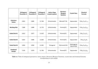
sample. However, the a-axes of both WD and the powdered sample did not agree with
literature values of 𝑌𝐵𝑎2 𝐶𝑢3 𝑂7 (and therefore, the graphs). Bizarrely, the a-axis length
obtained from the experiment was exactly twice that of the literature value. Further
research into the crystalline structure of 𝑌𝐵𝑎2 𝐶𝑢3 𝑂6.5 indicated that the value of the a-
axis length obtained via X-Ray diffraction was not as peculiar as first thought, as it agreed
with the accepted literature value, demonstrated below in figure 5.1.
Figure 5.1: Diagram of 𝑌𝐵𝑎2 𝐶𝑢3 𝑂6.5 whereby the a-axis is twice the length of the b-axis
[50].
Figure 4.6 demonstrates the relationship between the occupancy of the O(1) and O(5) sites
and the Oxygen deficiency of the lattice; reference 50 states that neutron scattering
reveals that the Oxygen deficit is more prominent in the 𝐶𝑢𝑂4 square planes, rather than
the 𝐶𝑢𝑂5 pyramid planes. Although a literature search on this alternative site deficit was
unsuccessful, it may offer an explanation as to why the a-axis in 𝑌𝐵𝑎2 𝐶𝑢3 𝑂6.51 and
𝑌𝐵𝑎2 𝐶𝑢3 𝑂6.5 is abnormally large (according to figure 4.5a, as this graph clearly states that
the a-axis is shorter than the b-axis for all Oxygen deficits for orthorhombic structures).
Regardless of the explanation, these orthogonal parameter lengths remain coherent with
those required for an orthorhombic lattice structure (𝑎 ≠ 𝑏 ≠ 𝑐).
A possible explanation for how these peculiar lattice parameter lengths allow
superconductivity in 𝑌𝐵𝑎2 𝐶𝑢3 𝑂6.51 and 𝑌𝐵𝑎2 𝐶𝑢3 𝑂6.5 is that YBCO structures with 𝛿 ≈ 0.5
have been known to possess ortho-II phases, whereby ortho-I denotes the normal
orthorhombic phase at 𝛿 = 0 and ortho-II denotes a structure of alternating Cu-O-Cu and
Cu-Cu chains in the basal plane. The possible significance of the ortho-II phase is that the
charge transfer from the 𝐶𝑢𝑂 to the 𝐶𝑢𝑂2 planes (discussed in chapter 2.6) take place only
if the ordered domains [64] (orthogonal parameters) are of an appropriate size. 𝐶𝑢𝑂2 planes
become superconducting if a significant amount of charge carriers are transferred from
the 𝐶𝑢𝑂 planes, which may only occur if the distance between Copper atoms in the 𝐶𝑢𝑂2
planes are preferable to the distance between 𝐶𝑢𝑂 planes. Perhaps the large a-axis
provides a situation in which the distance between Copper atoms is indeed preferable to
the distance between 𝐶𝑢𝑂2 planes in 𝑌𝐵𝑎2 𝐶𝑢3 𝑂6.51 and 𝑌𝐵𝑎2 𝐶𝑢3 𝑂6.5.

33. 32
5.5 Critical Temperature
This leads to the dependence of critical temperature on the Oxygen deficit of the
YBCO crystal lattice; Figure 4.4 is a plot of critical temperature as a function of Oxygen
defects. According to the graph, a superconducting sample of YBCO with 𝛿 = 0.49 or 𝛿 =
0.5 should have a critical temperature of approximately 56 K [64], which is far lower than
the critical temperature of the samples used in the experiment, which must have been at
least 77 K. Unfortunately an explanation for this peculiar outcome was not determined.
Research into the peculiar nature of the 58 K plateau yielded very interesting
theories; several experiments have shown [65] [66] [67] that there is an onset of 𝑇𝑐 > 0 for 𝛿 ≲
0.65, a plateau of 𝑇𝑐 ≈ 58 K for 0.35 ≲ 𝛿 ≲ 0.55 and a second plateau of 𝑇𝑐 ≈ 93 K for 𝛿 <
0.15. Beyond 𝛿 = 0.5 the critical temperature drops rapidly, reaching a value of 0 K at 𝛿 ≈
0.65. This range of compositions is comprised of broad superconducting transitions [61],
implying that the determination of the 0 K point is difficult. Jorgensen et al. suggests that
this may result from inhomogeneity in the samples, the severity of which increases with
higher Oxygen deficits. Poulsen et al. makes use of the anisotropic next-nearest-neighbour
lattice-gas (ASYNNNI) model together with the assumption that only minimal-size
clusters (MSCs) contribute to a charge transfer from the CuO planes by creating holes in
the 𝐶𝑢𝑂2 planes [68] (whereby holes are areas of positive charge). These clusters are
domains of coherent orthorhombic Oxygen orders of the ortho-I and ortho-II phases
mentioned above. The tendency of Oxygen atoms and vacancies to arrange themselves in
chains (rather than a random distribution across the lattice) leads to a varied Oxygen
order as a function of 𝛿, which implies that different orthorhombic symmetries occur at
different Oxygen deficits. Poulsen et al. suggests that the plateau observed between 𝛿 ≈
0.3 and 𝛿 ≈ 0.5 occurs due to a dynamic coexistence of both ortho-I and ortho-II
symmetries within these YBCO structures (perhaps in the form of a supercell) [61] [69].
5.6 Resistance
An attempt was made to measure the resistance across the working
superconducting disk; the experimental set-up involved Copper wires leading from a
multi-meter to the YBCO disk. Silver epoxy was applied to the disk’s surface as a
resistance-free substance for contact between the disk and the Copper wires, as is shown
in figure 5.2.
Figure 5.2: Image of Copper wires attached to WD using Silver epoxy (taped down, as
the Silver epoxy had recently dried and was still fragile).
The experiment was initially conducted with the disk at room temperature in order
to confirm that the set-up was working. Upon beginning the experiment it was found that

34. 33
the multi-meter was unable to produce a reading of resistance, implying that the wires
had failed to make Ohmic contact with the disk. Research into this matter revealed that
the process was a non-trivial one [70], and also yielded a particularly useful paper on the
subject which stated several different attempts to measure resistance across an YBCO
sample e.g. the use of a Nickel-based circuit repair glue, and several attempts at using
Silver epoxy [48]. Some of the resistance measurements performed during Safranski’s
experiment showed positive results, whereby the resistance would drop drastically as the
critical temperature of the YBCO sample was reached (cooling from the normal state to
the Meissner state). However, upon heating the sample from the Meissner state, an
abrupt increase in resistance was not measured – it is unclear as to whether the
experimental set-up or the sample was the cause of this anomaly. Some of their
measurements failed to demonstrate superconductive properties at all, but by the time
these runs had been performed, Safranski suggests that their samples had developed a
thin semiconducting layer of YBCO on the surface. Several attempts were made to cure
Silver epoxy at various temperatures and periods of time, suggesting once more that this
type of experiment was non-trivial. Admittedly, this part of the experiment was
abandoned due to the previously mentioned difficulties. Alternatively, an adaptation of
Safranski’s results was performed to demonstrate expected resistance measurements for
a superconducting material passing from its normal state to the Meissner state, which is
displayed below in figure 5.3, whereby the temperature measurements have been changed
from those used by Safranski (the results were erroneous, and not appropriate for the
samples used in the experiments performed for this report).
Figure 5.3: Adaptation of resistance/temperature graphs from Safranski’s paper to
demonstrate expected results [48], based on the information provided in chapter 4,
namely 𝑇𝑐 ≈ 58 𝐾 for YBCO with 𝛿 ≈ 0.5.
Evidently from figure 5.3, the resistance drops significantly and abruptly as the critical
temperature is reached, which agrees with theoretical expectations discussed in the
introduction.
A method of improving the investigation of resistance versus temperature would
be to use a four-wire resistance set-up, whereby a known electrical current would be
passed through a superconducting disk (above its critical temperature) through two of the
wires. The remaining two wires would be attached to the disk between the two current

35. 34
wires in order to measure the resistance (eliminating the resistance of the current wires).
The resistance would then be recorded as the temperature of the sample decreased below
its critical temperature. Additionally, a vacuum layer around the sample would increase
the accuracy of the temperature measurements (avoiding heat from the outside
environment interfering), which could also be applied to the Meissner and magnetic field
experiments. A layer of evaporated gold has also been suggested as a possibly reliable
method of achieving Ohmic contact [53].
5.7 Superconducting ring
As was briefly discussed in chapter 3, the powdered sample was intended for use
in a superconducting ring. The XRD results implied that the powdered sample was very
similar to that of WD, and that perhaps the powdered sample didn’t display any
superconductive properties during the Meissner experiments because it was insufficiently
compressed (whereby only sections of the sample would have become superconducting).
Upon further investigation, this superconductivity-related phenomenon was also
determined to be non-trivial, at which point it was realised that the appropriate
equipment for measuring minute changes in magnetic fields (namely SQUIDs) weren’t
readily available. Nevertheless, a literature search on the subject yielded two particularly
useful papers on the subject, both of which were particularly useful for chapter 2.5, one of
which outlines a sophisticated experiment on measuring the quantization of magnetic flux
within a superconducting ring system consisting of a high-temperature superconductor
(namely YBCO) connected to a low-temperature superconductor (namely Niobium) via
two ramp-type Josephson Junctions. The experiment involved the use of a SQUID to
measure minute changes in magnetic flux (induced by internal currents, which are
induced by an external, applied magnetic field) for 72 arrays of 0- and 𝜋- superconductor
rings, whereby 0- and 𝜋- indicate an increase (once induced) of an integer flux [𝑛Φ0] and
an increase of a half-integer flux [(𝑛 +
1
2
) Φ0], respectively. The experiment was also
performed in zero and non-zero background magnetic field environments, whereby the
Earth’s magnetic field was also accounted for. Bruel’s [39] measurements were positive
(with the exception of a few anomalies) and agreed with the expected results, which is
shown in figure 5.4.
Figure 5.4: Graph of measured values of magnetic flux (blue circles) in a 0-ring (without
a background magnetic field) compared with the expected steps in magnetic flux (solid
black lines) against an applied magnetic field [39].

36. 35
If the appropriate equipment were available, a magnetic flux experiment similar
to that performed by Bruel would have been attempted; rather than pressing the powder
into a pellet (or in this case, a ring), a hollow Aluminium toroid would have been
constructed, whereby the powdered sample would have been compressed within the
toroid. Following the format of the paper discussed above, an external magnetic field
would have been applied to the superconducting ring (below its critical temperature),
inducing a current within the material. This would then induce a magnetic field of its
own. An increase in the applied magnetic field would increase the current, but only in
quantized steps.
Due to a lack of appropriate equipment and delayed orders of working YBCO
samples, the experimental aspect of this report was somewhat hindered. Thankfully, an
important aspect of this report was to gain a detailed understanding of a range of
superconductivity theories, which was evidently achieved (considering chapter 2 and
explicit parts throughout chapter 5) during the time in which experiments couldn’t be
performed.
6. Conclusion
The main goals of this report were: to gain a firm understanding of several
theoretical aspects of the Yttrium Barium Copper Oxide structure and the phenomenon
known as Superconductivity; to observe the Meissner effect in a working superconducting
sample; to provide measurable evidence that the YBCO sample did in fact transition from
its Normal State to its Meissner state; and to suggest plausible reasons for any structural
differences between the working and failed YBCO samples, as well as how these
differences give rise to (or disallow) superconductivity.
Several theoretical aspects of Superconductivity were discussed in Chapter 2, one
of which was the Meissner effect; the characteristics of this phenomenon were discussed,
such as the expulsion of magnetic flux from inside the YBCO structure as it transitioned
from its Normal state to its Superconducting State. The Ginzburg-Landau theory was also
studied, particularly how it may be used to derive the London equations (which are
quantitative expressions of the Meissner effect), demonstrating that the Meissner effect
can be described by GL theory and that the London equations are in fact a consequence
of the coherence of a quantum state. The BCS theory was investigated, namely the theory
that charge carriers consist of Cooper pairs. The structural properties of YBCO were
discussed, most important of which was the relationship between the lattice parameters
and superconductive properties with the Oxygen defects of the crystal lattice.
The Meissner effect was successfully observed in a superconducting disk-shaped
sample of 𝑌𝐵𝑎2 𝐶𝑢3 𝑂6.51, but was not observed in any of the other disk samples or the
powdered sample. The magnetic field of a rare-Earth magnet was measured with and
without the inclusion of the YBCO disk, to determine whether the disk had any effect on
the magnetic field strength immediately outside the disk. It was proposed that the
magnetic field immediately outside the YBCO disk increased while the magnetic field of
the rare-Earth magnet decreased (indicating an expulsion of magnetic flux from the
YBCO sample), resulting in a ‘plateau’ in the magnetic field measurements.
Different chemical formulae and Oxygen defects were observed in the various
YBCO samples through the use of X-Ray diffraction. It was also determined that there
were differences in the orthogonal parameters of each sample. The a-axis of the working

37. 36
sample, according to graphs that demonstrated the relationship between orthogonal
parameter lengths and Oxygen defects, seemed to be abnormally large; twice the length
of the b-axis, in fact. However, further research showed that this parameter length was
typical of YBCO structures with 𝛿 ≈ 0.5. A possible explanation for this lattice parameter
length and for how Superconductivity, regardless of the lack of ‘ideal’ lattice parameter
lengths, nevertheless occurs in 𝑌𝐵𝑎2 𝐶𝑢3 𝑂6.51 were developed.
The relationship between the critical temperature of a YBCO sample with its
Oxygen deficiency was also investigate (to a smaller degree), and an explanation for the
peculiar plateau at 𝑇𝑐 ≈ 58 K involving a mixed, dynamic ‘super-cell’ state of ortho-I and
ortho-II lattice symmetries was considered.
An attempt was made to measure the resistance across the working YBCO disk
while it was above its critical temperature (in order to determine whether the apparatus
set-up was functioning). The attempt was unsuccessful due to the non-triviality of making
Ohmic contact between the superconductor surface and the Copper wires. Research into
the matter yielded a particularly useful paper, which outlined several attempts to make
Ohmic contact with superconducting samples, whereby some of the resistance
measurements yielded negative or anomalous results, further reinforcing the idea that
achieving Ohmic contact is difficult.
A superconducting ring-system was proposed for a magnetic flux experiment, but
was abandoned due to a lack of appropriate equipment and the non-triviality of this sort
of experiment. One paper in particular reinforced this, as well as provided an outline of a
sophisticated experiment, the basics of which (as well as the positive results) were
discussed as a possible method of performing the experiment.
There are several ways in which the experiments performed in this study could be
improved e.g. the addition of a vacuum layer during experiments involving temperature
measurement. Another possible improvement would be to keep the temperature of the
YBCO disk as low as possible for as long as possible; a comparison of the magnetic field
measurements with and without the YBCO disk were somewhat hindered due to the
temperature of the systems increasing above the critical temperature at different times.
A four-wire resistance system and an evaporated Gold layer were considered as methods
of improving the resistance experiment and to achieve Ohmic contact. The experimental
procedures of the discussed magnetic flux experiment were considered as a basis upon
which a smaller scale experiment could be performed (provided that the appropriate
equipment would be available next time), whereby a YBCO/Aluminium toroid system
would be subjected to magnetic fields of increasing magnitude below its critical
temperature.
The next possible step in research would be to perform similar experiments on low-
temperature superconductors, whereby the theories discussed in this report are more
applicable. Another fascinating phenomenon upon which research could be conducted is
persistent currents; perhaps an experiment in which a superconducting ring (below its
critical temperature) with a persistent current is monitored over a limited period of time
to determine decay (if at all) in the magnitude of the current.

38. 37
7. Acknowledgments
I’d like to thank Mr David Bradbury, my Lab Partner and friend, for his assistance
and patience during this report, and for his contribution to the plotted graphical data and
to figures 3.1 and 3.3. I am also grateful to Dr Dave Langstaff, Senior Experimental
Officer, for providing us with the required experimental apparatus, for his avidity to
helping with the Meissner experiments and for his suggestions of how to overcome some
of the experimental obstacles that were encountered.
I’d also like to thank Dr Martin Wilding, Senior Lecturer and our Project
Supervisor, for his guidance, especially on the YBCO structure and the significance of
Oxygen defects, and for his encouraging nudges in the right direction in terms of research
required for this report.
8. References
[1] M. Neeraj; Applied Physics for Engineers; PHI Lerning Private Ltd.; pp. 931, 19.2;
ISBN – 8120342429 (2011)
[2] P.J. Ford, G.A. Saunders; The Rise of the Superconductors; 1, 5; CRP Press; ISBN
9780748407729 (2004)
[3] H. K. Onnes; Akad. van Wetenschappen (Amsterdam); Vol. 14, pp. 113, 818 (1911)
[4] Blakemore, J.S.; Solid State Physics (Second Edition); Cambridge University Press,
Cambridge; pp 266, 3.6; ISBN – 0-521-30932-8 (1985)
[5] D. Saint-James, G. Sarma, E. J. Thomas; Type II superconductivity; Pergamon Press;
Headington Hill, Oxford; 13-14, 1.7; ISBN 00801239299780080123929 (1969)
[6] http://en.wikipedia.org/wiki/Yttrium_barium_copper_oxide
[7] M. Tinkham, Introduction to superconductivity, 2nd ed., McGraw-Hill, (1996)
[8] W. Meissner, R. Ochsenfeld; Ein Neuer Effekt bei Eintritt der Supraleitfähigkeit,
Naturwissenschaften, Vol. 21, pp. 787-788 (1933)
[9] A. D. C. Grassie; The Superconducting State; 5, 1.2; Sussex University Press, Sussex;
ISBN 0856210145 (1975)
[10] Edward M. Purcell, David J. Morin; Electricity and Magnetism (Third Edition);
Harvard University, Massachusetts; Cambridge University Press; 197, 4.4; ISBN 978-1-
107-01402-2 (2013)
[11] T. Van Duzer, C. W. Turner; Principles of Superconductive Devices and Circuits; 31-
35, 1.10; ISBN 0-7131-3432-1 (1981)
[12] J. E. Hirsch; Dynamic Hubbard model: kinetic energy driven charge expulsion, charge
inhomogeneity, hole superconductivity and Meissner effect; 9, 12; Institute of Physics
Publishing; Phys. Scr. 88, 035704 (16pp) (2013)
[13] A. Durrant; Quantum Physics of Matter; Institute of Physics Publishing, London;
ISBN 0750307218 (2000)

39. 38
[14] Michael Tinkham; Introduction to Superconductivity (Second Edition); McGraw-Hill
Book Co., New York; ISBN-13: 978-0-486-43503-9 (1996)
[15] Kittel, Charles; Introduction to Solid State Physics; John Wiley & Sons; pp. 273–
276; ISBN 978-0-471-41526-8 (2004)
[16] L. P. Gor’kov; Microscopic Derivation of the Ginzburg-Landau equations in the
Theory of Superconductivity; Soviet Physics JETP, Vol. 36 (9), No. 6; Institute of Physical
Problems, Academy of Sciences, U.S.S.R. (1959)
[17] P. C. Hohenberg, A. P. Krekhov; An introduction to the Ginzburg-Landau theory of
phase transitions and nonequilibrium patters; 23, 7 (2014).
- A link to reference 17: http://physics.nyu.edu/~pch2/GL_theory-submitOct13-
2014.pdf
[18] A. D. C. Grassie; The Superconducting State; 49, 3.1; Sussex University Press,
Sussex; ISBN 0856210145 (1975)
[19] V. L. Ginzburg; On the Superconductivity and Superfluidity (Nobel Lecture); P. N.
Lebedev Physics Institute, Moscow (2003)
[20] A. D. C. Grassie; The Superconducting State; 51, 3.1; Sussex University Press,
Sussex; ISBN 0856210145 (1975)
[21] V. L. Ginzburg; On the Theory of Superconductivity; Il Nuovo Cimento, Vol. 11, N. 6;
P. N. Lebedev Physics Institute, Moscow (1955)
[22] Lecture Notes on the Ginzburg-Landau Theory at Cambridge University,
Cambridge
A link to reference 22: http://www.qm.phy.cam.ac.uk/teaching/lecture_2_12.pdf
[23] F. London; On the Problem of the Molecular Theory of Superconductivity; Phys. Rev.
74, 562 (1948)
[24] A. A. Abrikosov; Type II Superconductors and the Vortex Lattice (Nobel Lecture);
Material Science Division, Argonne National Laboratory, USA (2003)
[25] Blakemore, J.S.; Solid State Physics (Second Edition); Cambridge University Press,
Cambridge; pp 277-288, 3.6; ISBN – 0-521-30932-8 (1985)
[26] H. Fröhlich; Theory of the Superconducting State. I. The Ground State at the
Absolute Zero of Temperature; Phys. Rev. Vol. 79, 3 (1950)
[27] C. A. Reynolds, B. Serin, W. H. Wright, L. B. Nesbitt; Superconductivity of Isotopes
of Mercury; Phys. Rev. 78, 487 (1950)
[28] E. Maxwell; Isotope Effect in the Superconductivity of Mercury; Phys. Rev. 78, 477
(1950)
[29] J. Bardeen; Electron-Phonon Interactions and Superconductivity (Nobel Lecture);
Department of Physics and of Electrical Engineering, University of Illinois, Urbana,
Illinois (1972)

40. 39
[30] A. D. C. Grassie; The Superconducting State; 27, 2.2; Sussex University Press,
Sussex; ISBN 0856210145 (1975)
[31] J. Bardeen, L. N. Cooper, J. R. Schrieffer; Theory of Superconductivity; Phys. Rev.
Vol. 108, 5 (1957)
[32] L. N. Cooper; Bound Electron Pairs in a Degenerate Fermi Gas; Phys. Rev. Vol. 104,
4 (1956)
[33] D. Saint-James, G. Sarma, E. J. Thomas; Type II superconductivity; Pergamon Press;
Headington Hill, Oxford; 44-45, 3.3; ISBN 00801239299780080123929 (1969)
[34] R. Doll, M. Näbauer; Experimental Proof of Magnetic Flux Quantization in a
Superconducting Ring; Phys. Rev. Lett 7, 52 (1961)
[35] F. London; Superfluids, Vol 1, Macroscopic Theory of Superconductivity; John Wiley
& Sons, Inc., London (1950)
[36] L. I. Schiff; Quantum Mechanics (third edition); 31, 2; McGraw Hill, New York (1968)
[37] S. Gasiorowicz, Quantum Physics, 3rd ed., John Wiley and Sons, Inc., (2003)
[38] R. Bruel, A. Timmermans; Magnetic Flux Quanta in High-Tc/Low-Tc Superconducting
Rings with π-phase-shifts (Bachelor Thesis); University of Twente (2013)
[39] A. D. C. Grassie; The Superconducting State; 70, 3.7; Sussex University Press,
Sussex; ISBN 0856210145 (1975)
[40] G. van der Steenhoven et al.; Fractional Flux Quanta in High- 𝑇𝑐/Low- 𝑇𝑐
Superconducting Structures, Ph.D. Thesis, University of Twente; Gildeprint
Drukkerijen; ISBN 978-90-9024316-0; C.J.M. Verwijs (2009)
[41] L. Onsager; Magnetic Flux through a Superconducting Ring; Phys. Rev. Lett. 7, 50
(1961)
[42] B. S. Deaver, W. M. Fairbank; Experimental Evidence for Quantized Flux in
Superconducting Cylinders; Phys. Rev. Lett. 7, 43 (1961)
[43] H. Wenk, A. Bulakh; Minerals: Their Constitution and Origin; New York, NY:
Cambridge University Press; ISBN 978-0-521-52958-7 (2004)
[44] M. T. Dove; Structure and Dynamics (An Atomic View Of Materials); 35-37, 2.4.1;
Oxford University Press; ISBN 978-0-19-850677-5 (2003)
[45] A. M. GGlazer; Simple Ways of Determining Perovskite Structures; 35-37, 2.4.1; Acta
Cryst. A31, 756 (1975)
[46] D. M. Buitrago, N. C. Reyes-Suarez, J. P. Peña, O. Ortiz-Diaz, J. Otálora, C. A. Parra
Vargas; High Temperature Superconductivity on the New Superconductor System
𝑌𝑏1.8 𝑆𝑚1.2 𝐵𝑎5 𝐶𝑢8 𝑂18; J. Supercond Nov Magn, 26:2269-2271; Springer Science+Business
Media (2013)
[47] Crystal Structure of YBCO; Hoffman Lab; Harvard University;
http://hoffman.physics.harvard.edu/materials/Cuprates.php

41. 40
[48] Chris Safranski; Resistance of the Superconducting Material YBCO; Senior Project
presented to The Faculty of the Department of Physics, California Polytechnic State
University, California (2010)
[49] K. A. Miller; The Unique Properties of Superconductivity in Cuprates; J Supercond
Nov Magn 27:2163-2179; Springer Science+Business Media (2014)
[50] A. K. Saxena; High-Temperature Superconductors: Crystal Structure of High
Temperature Superconductors; 2, 224; Springer Series in Material Science; ISBN 978-3-
642-00711-8 (2010)
[51] Small article on YBCO. Unfortunately, no author was available
- Link to reference [53]; http://www.ch.ic.ac.uk/rzepa/mim/century/html/ybco.htm
[52] D. Varshney, G. S. Patel, S. Shah, R. K. Singh; Pairing mechanism and
superconducting state parameters in 𝑌𝐵𝑎2 𝐶𝑢3 𝑂𝛿; Indian Journal of Pure and Applied
Physics, Vol. 39, pp. 246-258 (2001)
[53] I. Kirschner, J. Bánkuti, M. Gál, K. Torkos, K. G. Sólymos, G. Horváth; High-Tc
Superconductivity in La-Ba-Cu-O and Y-Ba-Cu-O Compounds; Europhys. Lett., 3 (12), pp.
1309-1314 (1987)
[54] V. Z. Kresin, S. A. Wolf, H. Morawitz; Mechanisms of conventional and high-Tc
superconductivity; Oxford University Press, New York (1993)
[55] J. Bardeen, L. N. Cooper, J. R. Schrieffer; Microscopic Theory of Superconductivity;
Phys Rev. 106, Sov Phyics JETP. 11 (1960)
[56] A. Lanzara, P. V. Bogdanov, X. J. Zhou, S. A. Kellar, D. L. Feng, E. D. Lu, T. Yoshida,
H. Eisaki, A. Fujimori, K. Kishio, J.-I. Shimoyama, T. Noda, S. Uchida, Z. Hussain & Z.-
X. Shen; Evidence for ubiquitous strong electron–phonon coupling in high-temperature
superconductors; Nature 412, 510-514 (2001)
[57] L. K. Miodrag; Importance of the Electron–Phonon Interaction with the Forward
Scattering Peak for Superconducting Pairing in Cuprates; Journal of Superconductivity
and Novel Magnetism, Vol. 19, Nos. 3-5 : Springer Science + Business Media, Inc (2006)
[58] F. Marsiglio, J. P. Carbotte; Electron-Phonon Superconductivity; Cornell University
Library (2008)
[59] J. G. Bednorz, K. A. Müller; Possible High Tc Superconductivity in the La-La-Cu-O
System; Z Phys. B – Condensed Matter 64, 189-193 (1986)
[60] J. G. Bednorz, K. A. Müller; Perovskite-type oxides – The new approach to high-Tc
superconductivity; Review of Modern Physics, Vol. 60, No. 3 (1988)
[61] J. D. Jorgensen et al.; Structural properties of oxygen-deficient 𝑌𝐵𝑎2 𝐶𝑢3 𝑂7−𝛿; Phys.
Rev. B, Vol 43, 4 (1989)
[62] S. Davison et al.; Chemical problems associated with the preparation and
characterization of superconducting oxides containing copper; Chemistry of high-
temperature superconductors, American Chemical Society p. 65-78 (1987)

42. 41
[63] X. L. Xu, J. D. Guo, Y. Z. Wang, A. Sozzi; Synthesis of nanoscale superconducting
YBCO by a novel technique; Physica C 371, 129-132 (2002)
[64] T Zeiske et al.; On the Structure of the Superconducting Ortho-II Phase of
𝑌𝐵𝑎2 𝐶𝑢3 𝑂6.51; Journal of Electronic Materials, Vol. 22, No. 10 (1993)
[65] R. J. Cava, et al.; Superconductivity in Multiple Phase Sr2Ln1–xCaxGaCu2O7 and
Characterization of La2–xSrxCaCu2O6+δ; Physica C. 185-189, p. 180-183
[66] R. J. Cava, et al.; STRUCTURAL ANOMALIES, OXYGEN ORDERING AND
SUPERCONDUCTIVITY IN OXYGEN DEFICIENT Ba2YCu3Ox; Physica C. 165, 419-
433 (1990)
[67] V. I. Simonov; Atomic Structure and Physical Properties of Crystals; Institute of
Crystallography, USSR Acad. Sci., Moscow [Butll. Soc. Cat . Cien.], Vol. XII, Num. 2
(1991)
[68] J. D. Jorgensen et al.; Oxygen ordering and the orthorhombic-to-tetragonal phase
transition in YBa2Cu3O7-x; Phys Rev B, Vol. 36, 7 (1987)
[69] R. Beyers et al. Oxygen ordering, phase separation and the 60-K and 90-K plateaus
in 𝑌𝐵𝑎2 𝐶𝑢3 𝑂𝑥; Nature 340, 619-621 (1989)
[70] J. W. Ekin; Ohmic Contacts to High- 𝑇𝑐 Superconductors; Proc. SPIE 1187, Processing
of Films for High Tc Superconducting Electronics, 359 (1990)
9. Literature Review
High Temperature Superconductivity
1. Introduction
The project is a study of the nature of superconductive materials.
Superconductivity is a quantum mechanical phenomenon of the expulsion of the magnetic
field from the material, and the state in which the material has zero electrical DC
resistance. This occurs when the material is cooled to very low temperatures (below the
characteristic critical temperature of the particular material).
Superconductivity was first observed in 1911 by Dutch physicist Heike
Kamerlingh Onnes. While cooling a solid mercury wire to approximately 4 Kelvin (-2690C)
using Liquid helium, Onnes observed that the resistance in the wire disappeared very
suddenly. Onnes’ work earned him the Nobel Prize in physics just two years later. The
next milestone in understanding how matter behaves at these extreme temperatures
occurred in 1933; German physicists Walther Meissner and Robert Ochsenfeld discovered
superconducting materials repel magnetic fields. It was observed that the currents
induced in the superconductor exactly mirror the external magnetic field, which would
otherwise have penetrated the material. The phenomenon is known as strong
diamagnetism but is today often referred to as the “Meissner Effect.” This effect is
sufficiently strong to levitate a magnet over a superconducting material (in the
superconducting state).

43. 42
Fritz and Heinz London explained the Meissner Effect in 1935 with (what are now
known as) the London equations, stating that the effect occurred due to a minimization of
electromagnetic free energy carried by superconducting current. In 1950, Vitaly Ginzburg
and Lev Landau devised what is known today as the Ginzburg-Landau theory. The theory
had great success explaining the macroscopic properties of a superconductor, and also
provided categories in which superconductors may be divided into i.e. Type I and II. 1957
saw perhaps the most important theory for superconductivity, the Bardeen Cooper
Schrieffer (BCS) theory. Developed by John Bardeen, Leon Cooper and John Robert
Schrieffer, the theory gives a complete microscopic explanation of superconductivity and
describes the superconducting current as a superfluid of Cooper pairs (pairs of electrons)
that are interacting with phonons, which earned them the Nobel Prize in physics in 1972.
Since the discovery of superconductivity there have been numerous metals and alloys that
have displayed the phenomenon, but all at very low temperatures. In 1986 however, Georg
Bednorz and Karl Alexander Mueller discovered superconductivity in a lanthanum-based
cuprate perovskite material at 35K. This clearly differed from the critical temperature of
conventional superconducting materials; the discovery began an age of ceramic
superconductor production with much higher critical temperatures (which the BCS theory
cannot fully explain). These transition temperatures have increased to greater than that
of the boiling point of liquid nitrogen, meaning that experimentally it is much easier to
demonstrate superconductivity. Further research has seen superconductivity in organic
materials such as fullerenes and ever increasing transition temperatures in new
materials. In 2014 the phenomenon was observed at room temperature [1] (albeit for a
millionth of a second).
Figure 1.1: Image of a magnet levitating over a superconductor [2].
There are several useful applications for superconductivity; in transport, the
magnetic levitation can be used for vehicles such as trains, which float above the tracks.
The advantage of this method rather than conventional electromagnets is that there is no
energy lost as heat due to an absence of friction between the train and the tracks. The
most well-known example of this method of transport is the MAGLEV train in Japan,
which can reach speeds of up to 361 miles per hour. Another very important use for
superconductors is MRI (Magnetic Resonance Imaging) scanners. Inside the scanner, the
human body is subjected to a strong superconductor-derived magnetic field which forces
hydrogen atoms in the water and fat molecules to accept energy. This energy is then
released and a computer can detect this energy at a certain frequency and display the
results graphically. Superconducting magnets are used in the CERN Large Hadron
Collider which makes the acceleration of sub-atomic particles to near light speed possible.

44. 43
Figure 1.2: Image of a brain scan produced by a MRI scanner [3].
We will discuss the nature of superconductivity in a material known as Yttrium Barium
Copper Oxide; a material with a perovskite-like structure that displays High-temperature
superconductivity. During this experiment, we will attempt to address three major
questions on the nature of high temperature superconductivity (SC), and SC in general:
An attempt will be made to demonstrate and explain the Meissner effect in our sample
of YBCO; The Meissner effect being the spontaneous expulsion of a superconducting
material’s magnetic field as the material’s temperature is reduced below its critical
temperature (while exposed to a weak magnetic field). The material becomes perfectly
diamagnetic, which cancels all magnetic flux within the material – the material never
has an internal flux density, even when placed within an applied magnetic field. [4]
The effect will be discussed in more detail in the theory section of this review.. If the
Meissner effect occurs, it will be apparent; a magnet will be placed above the
superconducting material – if it floats above the material, then the material has
expelled all of its magnetic field.
An attempt will be made to explain how defects within the YBCO structure
affect/determine the superconductive properties of the material below the critical
temperature. The first step in achieving an understanding of this is to produce a three-
dimensional picture of the density of electrons (from which we can determine the
structure and its defects) by means of X-ray Diffraction; the picture of an YBCO
sample with defects will be compared with that of an YBCO sample without defects.
The superconductive properties of both samples will be examined, and the data
obtained will be analysed in an attempt to determine how Oxygen defects affect
superconductivity.
An attempt will be made to demonstrate zero resistance within the YBCO sample, and
to explain why it arises. This will be done by placing probes within the copper block,
which will read the resistance of the material. This characteristic will be discussed in
the theory section.
An attempt will be made to determine if current flux is quantized; this will be done by
producing a superconducting ring system for a powdered sample of YBCO. The ring
will be subject to an external magnetic field while below its critical temperature. An
increase in the external magnetic field should result in an increase in magnet flux in
quantized steps.
2. Theory
2.1. Superconductors

45. 44
Superconductors are materials that lose all resistance to the flow of electric current
when their temperature is dropped below their critical temperature. Besides achieving
zero resistance below their critical temperature, superconductors gain other magnetic and
electrical properties, such as zero resistivity; if the resistivity drops to 0, then the
resistance of the material will also drop to zero, which gives rise to the existence of
permanent currents. [5] Another example superconductive material properties is a sudden
change in magnetic susceptibility from a paramagnetic value to -1, meaning the material
has become perfectly diamagnetic. Diamagnetic materials are materials that create and
induced magnetic field in the opposite direction of an external magnetic field, which
causes a repulsion effect. This is known as the Meissner effect. Both of these properties
will be discussed and demonstrated during the experiment.
Figure 2.1.1: diagram demonstrating the exclusion of a magnetic field (represented as
arrows) from a superconducting material below the critical temperature [6].
Figure 2.1.2: diagram representing the sharp drop in resistance (due to the drop in
resistivity) of a superconductor at the critical temperature, compared to a non-
superconducting material [7].
2.1.1. Types of Superconductors
There are several methods of classifying superconductors. One such example is
how the material responds to a magnetic field; if the magnitude of an external magnetic

46. 45
field is increased beyond the critical point (which is dependent upon the material) the
magnetic flux penetrates the material. The material will thus undergo a phase transition
from a superconducting state to a normal state.
In Type I superconducting materials, the material continues to expel magnetic flux
until the magnetic field exceeds the critical point (Hc). At which point, the material
abruptly switches from a Meissner state to a normal state. Type I superconductors are
usually pure materials.
Type II semiconducting materials act as type I superconductors in a weaker
magnetic field than that of the material’s critical field. If the external magnetic field is
increased above the critical point (Hc1), then the material transitions into the ‘mixed-
state’, which is a state of partial penetration of magnetic flux. By further increasing the
magnetic field, the flux penetration of the material will increase to a maximum at upper
field strength (Hc2), whereby the material transitions to the normal state. Type II
superconductors are usually alloys.
Figure 2.1.3: Image of the critical magnetic field strengths of type I and type II
superconductors, where the larger triangle represents the abrupt switch from the
Meissner state to the normal state of type I, and the smaller triangle represents the
transition to the vortex state of type II [8a].
2.1.2. High Temperature Superconductors
Superconductors may also be categorised by their critical temperature; low-
temperature superconductivity and high-temperature superconductivity, which are
materials that transition to the superconductive state below and above 30 K, respectively.
The benefit of high-temperature superconductors is that liquid nitrogen can be used as a
coolant. YBCO is an example of a high-temperature superconductive material, and the
importance of the perovskite structure to superconductivity will be discussed further in
the theory section. High-temperature superconductivity is not fully understood; there is
no theory that is generally accepted to sufficiently explain high-temperature (HT)
superconductivity. Many scientists believe that the coupling between electrons and
phonons (or lattice vibrations) induces electron pairing within HT superconductors, but
there is a lack of direct evidence. [9]
2.2. Meissner Effect
The Meissner effect is a phenomenon whereby the magnetic field of a
superconductor gets expelled as it transitions into the superconducting state. Nearly all
the magnetic flux is expelled from a superconductor in a weak, applied magnetic field.
Electric currents form near the surface and the magnetic field of these surface currents
cancels the weak applied field. The expulsion of the field doesn’t change with time,

47. 46
therefore the currents are persistent. The Meissner effect cannot be explained by infinite
conductivity alone; a concise explanation was first given by the London equations.
Superconductors that experience the Meissner effect exhibit super diamagnetism.
This means that the total magnetic field deep inside the material is zero, and that their
magnetic susceptibility, =-1. In superconductors the origins of the diamagnetism is
different to what is observed in normal materials. In a superconductor, an illusion of
perfect diamagnetism is seen from the persistent currents on the surface which oppose
the applied field.
The original paper [10] by Meissner and Ochsenfeld is in German which is of little
use to us, but there is plenty of literature on the Meissner effect. The book Introduction
to Solid State Physics [11] by Charles Kittel gives a thorough description of the Meissner
effect (and other theories relating to superconductivity).
2.3. London Equation
The London equation shows the relationship between electromagnetic fields and current,
in and around a superconductor.
𝒋 𝒔 = −
𝑛 𝑠 𝑒2
𝑚𝑐
𝑨
Whereby js is superconducting current density, e is the charge of an electron and proton, m
is the electron mass, ns is a constant associated with a number density of superconducting
carriers, and A is the vector potential (introduced by the London brothers).
Also predicted was a characteristic length scale, λ;
∇2
𝑩 =
1
𝜆2
𝑩
Whereby
𝜆 ≡ √
𝑚𝑐2
4𝜋𝑛 𝑠 𝑒2
𝜆 is known as the London penetration depth. This shows that the magnetic field inside
the superconductor decays exponentially. The London penetration depth varies depending
on the material. The Electromagnetic Equations of the Supraconductor [12] by F. and H.
London gives a very detailed derivation of the London equation and how it explains the
Meissner effect, while High Temperature Superconductivity [13] by Gerald Burns gives a
more concise derivation, which is much easier to grasp. The book also gives an excellent
overview of many aspects that this literature review covers.
2.4. Ginzburg-Landau Theory
The Ginzburg-Landau theory is a mathematical physical theory used to describe
superconductivity. It postulated a model to describe type I superconductors without
looking at the microscopic properties.
The Ginzburg-Landau theory predicted new characteristic lengths in a superconductor.
The first is called the coherence length, represented by the symbol, ξ. For a temperature

48. 47
greater than the critical temperature of the superconductor, the coherence length is given
by;
For a temperature below the critical temperature, the coherence length is given by;
The second characteristic length is the penetration depth; previously show with
the London equations. The equation below shows the penetration depth (λ) in terms of the
Ginzburg-Landau model;
The Ginzburg-Landau parameter “k” is the ratio between penetration depth and
coherence length (λ/ξ). Type 1 super conductors have a k value between 0 and 1/√2 and
type 2 superconductors have a k value greater than 1/√2. The Superconducting State [14]
by A.D.C. Grassie goes into great detail with the Ginzburg Landau theory, its equation,
and relationship with coherence length and penetration depth. The mathematical side of
the theory is very complicated and perhaps goes into too much depth for our experiment.
2.5. BCS Theory
BCS theory was the first microscopic theory of superconductivity. The microscopic
effect is the condensation of Cooper pairs into a boson-like state. A Cooper pair is a pair
of electrons which are bound together in a certain way at low temperatures. There is an
arbitrarily small attraction between electrons that can create a paired state which has
energy below that of the Fermi energy, which implies that they are bound. In
superconductors the attraction is caused by the electron-phonon interaction. The energy
of the pairing interaction is around the order of 10-3eV and these pairs can break with
thermal energy, so there are a significant number of electrons in Cooper pairs at low
temperatures. Materials with heavier ions have lower transitioning temperatures. The
theory of Cooper pairing explains this; heavier ions are harder to move and less able to
attract electrons, giving a smaller binding energy. If the temperature is low enough,
electrons become unstable against forming into Cooper pair near the Fermi surface. The
binding occurs in an attractive potential, no matter how weak. In superconductor the
attraction is usually due to an electron-lattice interaction. The BCS theory itself doesn’t
require an origin of the potential, only that it is attractive.
The electron-phonon interaction in many superconductors arises from an electron
moving through a conductor, attracting nearby positive charges in the lattice. The lattice
deforms and causes another electron with opposite spin to move into the region of higher
positive charge density. The two electrons then become pairs, and in a superconductor,
there are a great number of these pairs. These pairs overlap and form a condensate; the
condensed state means that breaking one of the pairs would affect the entire condensate.
Therefore the energy to break a single pair is related to the energy needed to break all of

49. 48
the pairs. At low temperatures there are a small number of kicks from oscillating atoms
in the conductor, but because of the energy barrier that the condensate has formed, these
kicks do not affect the condensate. The electrons remain in pairs and resist the kicks and
therefore the electron flow through the superconductor will not experience resistance. The
BCS theory does not completely describe features of high-temperature superconductivity;
the threshold for the theory to hold is believed to be between 30 and 40K.
The Theory of Superconductivity [15] published by Bardeen, Cooper and Schrieffer
obviously goes into great detail about this theory and is useful as it explains what Cooper
pairs are; some aspects mathematically may go too deep for our needs. The book
mentioned previously by Gerald Burns also explains BCS theory and Cooper pairs very
well.
2.6. Josephson Effect
The Josephson Effect is a description of when a current flows indefinitely without
an applied voltage (super current) across a device known as a Josephson junction [16]. A
Josephson junction consists of two superconductors separated by a weak link. The weak
link can consist of a thin insulating barrier, a small section of non-superconducting metal
or a physical constriction which weakens the superconductivity at the point of contact.
The effect is a macroscopic quantum phenomenon where tunnelling of
superconducting Cooper pairs take place. The basic equations for the dynamics of the
Josephson Effect are;
𝑈(𝑡) =
ℏ
2𝑒
𝜕𝜙
𝜕𝑡
Which is known as the superconducting phase evolution equation, and
𝐼(𝑡) = 𝐼𝑐 sin[𝜙(𝑡)]
Which is known as the Josephson current-phase relation whereby U(t) and I(t) is the
voltage and current across the junction, φ(t) is the phase difference across the junction, Ic
is the critical current of the junction (the critical temperature can be affected by
temperature as well as an applied magnetic field,) h/2e is the magnetic flux quantum
constant (inverse of the Josephson constant.)
There are three main effects:
1. The DC Josephson Effect
This is when a direct current crosses from the insulator where there is no external
electromagnetic field, leading to tunnelling.
2. The AC Josephson Effect
With a fixed voltage across the junctions, the phase changes linearly with time and
therefore the current would be an AC current.
The Josephson junction acts as a perfect voltage to frequency converter.
3. The Inverse AC Josephson Effect
When the phase takes a certain form, distinct AC voltages may carry DC current across
the junction and it acts as a perfect frequency to voltage converter.
The book Superconductivity [17] by Ginzburg and Andryushin has a detailed description of
this effect and its applications, such as SQUIDs. The paper titled The Meissner Effect and

50. 49
the Josephson Effect in Superconductors [17a] by Leo Zhou show the Josephson Effect
experimentally, which could be useful.
3. Experiment
This section highlights the importance of the literature search with the specific
theories and information required to carry out the experiment. Our primary goal is to
demonstrate the Meissner effect in our sample of YBCO. The Meissner effect is explained
in several books (as has been highlighted in the previous chapter). An interesting take on
the Meissner effect in ‘unconventional’ superconductors is the subject of the paper The
origin of the Meissner effect in new and old superconductors, whereby superconductivity
is driven by holes (rather than electrons in the ‘conventional’ cases) and an outward flow
of negative charge induced by an internal electric field. The paper also argues that while
the BCS theory and the London effect do not accurately predict superconductivity in HT
superconductors, aspects of them must be correct in order to accurately describe
superconductivity in LT superconductors, (which is useful, as many other papers have
failed to state this). [19]
Another paper that follows the idea of Hole Superconductivity is Charge
Expulsion, Spin Meissner Effect, and Charge Inhomogeneity in Superconductors; the
paper explains Hole Superconductivity to some degree, and then goes on to explain how
the Meissner effect arises from Hole Superconductivity in highly negatively charged
systems, such as cuprates and planes in iron arsenides. [20] The paper perhaps goes into
more detail that is required for our experiment (such as the explanation of the Spin
Meissner effect and complicated electrodynamics), but will still be useful.
The experiment will proceed as follows; the Yttrium Barium Copper Oxide sample
will be placed in an aluminium ring (in which resistance probes will be placed, to measure
the resistance of the sample once the Meissner effect has been observed), and liquid
nitrogen will be poured on to the sample to reduce its temperature below its critical
temperature. The Beijing International Conference on High Temperature
Superconductivity contains a paper which outlines an analysis of the copper valance in
cuprates, whereby it briefly mentions an experiment similar to the one that will be
performed for this report that measured the resistance of the sample using a four-probe
method, while the sample was fixed in an indium block. The paper has a useful description
of the importance of copper valency and oxygen content on the superconductive
characteristic of cuprate structures, stating that the movement of oxygen in and out of
the lattice is dependent on the valence state of the copper within the lattice, and that
there is a strong relationship between the critical temperature and the oxygen content.
The paper also states that the mechanism responsible for superconductivity in YBCO
systems remains clear, which seems evident from our attempt to search for concise
literature on the subject. [21]
Demonstrating the Meissner effect and zero resistance in a metal is a field of study
that may be studied (and subsequently mentioned in the report) if time allows it. The
induction of the Meissner effect in metals can be explained by the BSC theory (which is
mentioned in many papers, such as The origin of the Meissner effect in new and old
superconductors [19]. A useful paper; Explanation of the Meissner effect and prediction of
a spin Meissner effect in low and high Tc superconductors; explains how the Meissner
effect arises in conventional, metal superconductors (surface currents generating a
magnetic field antiparallel to the external magnetic field), but it also goes into greater
detail of how this phenomenon arises, stating that the conventional BCS theory does not
explain how Meissner currents are generated. The paper also touches on the tendency of
metals to expel negative charge when their conduction band has excess electrons (and
therefore negative charge), and how this condition implies that the physics behind HT

51. 50
(and LT) superconductivity is essentially the same for metals and cuprates alike. [22] The
paper does not go into great detail on the basics and generality of the Meissner effect (i.e.
how the Meissner effect can be applied to other materials), but if it is required that we
describe the Meissner effect in great detail, this paper will be useful.
Another major question that will hopefully be addressed is the quantisation of flux
in a ring of superconducting material; Flux quantization in a high-Tc superconductor is a
short but very useful paper that precisely outlines and experiment to determine the
quantization of flux in an Yttrium-based ceramic superconductor. The experiment
involves the use of liquid helium to cool a sintered ring of an Yttrium Barium Copper
Oxide sample (Y1.2Ba0.8CuO4) with a high critical temperature and the use of radio
frequency SQUIDs to measure the flux. Interestingly, the experiment suggests that the
quantisation of the flux is caused by cooper pairs (electrons, specifically), as in BCS
superconductivity conventionally observed in Low-Temperature superconductors [23],
which will be useful as a reference as an explanation for the quantisation of flux in our
reports.
4. Structure
This section highlights the importance of the literature search of the structures of
various materials, and how these structures give rise to superconductivity.
One of the main structures of interest is the perovskite structure. A material which
is said to have a perovskite structure has a crystal structure similar to that of Calcium
Titanium Tri-Oxide (CaTiO3). The general chemical formula is ABX3 where ‘A’ and ‘B’ are
cations of different sizes, and X is an anion, usually a Halogen. The ideal structure of a
perovskite material is a cubic unit cell, which consists of a primary cation in each corner
of the unit cell, another cation positioned at the centre of the unit cell, and an assortment
of anions at the face centred positions within the unit cell. This can be shown in the image
below; where the green and red orbs represent cations, while the blue orbs represent the
anions:
Figure 4.1: Image of the perovskite crystalline structure [24]
High temperature superconductivity is an example of an important technical
application of perovskites. Compounds such as Yttrium Barium Copper Oxide (YBCO)
were one of the first materials to show superconductivity above the boiling point of liquid
nitrogen (77K). Although the mechanism for why these structures demonstrate
Superconductivity at high temperatures is uncertain, it is believed to be related to the
planar layering of Copper Oxide within the structure (which will be discussed shortly,
along with the importance of defects on the structure of YBCO). Other research suggests

52. 51
that holes (positively charged vacancies with the lattice) of hypo-charged oxygen in the
charge reservoirs are responsible (which are also discussed shortly).
As a side note; YBCO has the potential to have one of two CuO planes; the chain
plane, or the square plane; the square plane is the plane in which superconductivity
originates. The Copper ions within the structure are also important because they
constitute the essential structure of the system. All copper oxide based superconductors
possess CuO2 layers, in which there are single cooper pairs (a pair of electrons that are
bound under low temperature conditions).
Figure 4.2: Illustration of the copper planes in an YBCO structure [8]
Another of our goals for this experiment is to appreciate the effect that defects have
on the superconductive characteristics of the YBCO. This will be done by using X-Ray
diffraction to determine and compare the structures of an YBCO material with no defects
and an YBCO material with defects, and to then compare their superconductive
properties.
YBCO has a distorted, oxygen deficient, multi-layered perovskite-like
orthorhombic structure, which possesses Copper Oxide layers, between which
superconductivity takes place. The configuration of Copper Oxide plays an important role
in the superconducting mechanism. Some particularly useful pieces of literature on the
subject of the perovskite and cuprate structures (particularly YBCO, but not excluding
other ceramic systems or oxides such as La-Ba-Cu-O or Bi-Sr-Ca-Cu-O) are CRYSTAL
STRUCTURES OF SOME HIGH-TEMEPRATURE SUPERCONDUCTORS [25] and High-
Tc Superconductivity in La-Ba-Cu-O and Y-Ba-Cu-O Compounds by [26]. The first paper
goes into great detail on the Copper oxide layers within the structure of YBCO, and briefly
outlines the role that oxygen vacancies, the chemical composition of the material, and
cation substitutions play in superconductivity. While this paper provides basic details of
the understanding of how the structure of YBCO induces superconductivity, and has
varied and useful diagrams of superconductive structures (which we may use as
references), it does not go into enough detail, although it is a good starting point. The
second paper attempts to address the various possible reasons of superconducting

53. 52
interactions, such as electron-phonon interactions (which seems to be mentioned often in
literature), but again, the literature fails to go into precise detail.
On the other hand, Evidence for ubiquitous strong electron–phonon coupling in
high-temperature superconductors [27] attempts to tackle this interpretation of
superconductivity, by suggesting that electron-phonon pairs can be interpreted at lattice
vibrations, which drives the formation of cooper pairs. The paper puts forwards a strong
case for phonons as a possible candidate for conventional superconductivity, but also
states that the electron-phonon interactions are a largely unexplored topic, and as such,
our possible inclusion of this theory will be brief. Another example of a paper in support
of the electron-phonon interactions (as opposed to the Hubbard Model or
antiferromagnetic spin fluctuations is Importance of the Electron–Phonon Interaction
with the Forward Scattering Peak for Superconducting Pairing in Cuprates [28]; the level
of physics described in this paper goes above and beyond what is required for our project,
but it will likely be used in a group of similar references to support to electron-phonon
interaction interpretation of superconductivity.
The origin of High-temperature superconductivity is not well understood, and our
literature search of the subject yielded little to no results. However, the University of
Maryland claim to have found evidence that the pairing of electrons by magnetic
excitations is the cause of HT superconductivity. [29]
Several papers have focused on the doping of perovskite structures and the substitution
of Yttrium for heavier earth-metals, but unfortunately these papers cover material that
is not particularly useful for our report.
High-temperature cuprate superconductors studied by x-ray Compton scattering and
positron annihilation spectroscopies [30] suggests that defects (such as Oxygen vacancies)
in crystal structures increase the critical temperature of the material, and the greater the
number of defects, the higher the critical temperature (to a limit), determined by the
equation
𝑘 𝑏 𝑇𝑐 𝜏~ℏ
Where 𝜏 is the electron relaxation time within the structure; by introducing more defects,
the electron scattering increases (𝜏 decreases) and Tc increase. Again, the paper lacks any
precise information on the nature of oxygen vacancies/holes, but provides a starting point
from which an understanding of the significance of defects in a superconducting material
can be developed.
An interesting phenomenon is that superconductivity arises in most metals, but
not all metals; it is believed that superconductivity arises due to the arrangement of atoms
within the structure of materials. In Superconductivity [31] it is suggested that
superconductivity arises in materials (which are made purely of a single element) whose
number of valence electrons per atom is greater than 2 or less than 10, and that the critical
temperatures of these materials depends on the arrangement of the crystal structure. A
table of superconducting materials is provided below;

54. 53
Table 4.1: table of elements, their critical temperatures and their lattice ‘systems’
This is not to say that metal elements that are not included in this graph cannot be made
superconducting; their transition to superconductivity is at such low temperatures that
require such high purities of the material, that superconductivity has not been
demonstrated conclusively.
5. References
[1] R. Mankowsky, A. Subedi, M. Först, S. O. Mariager, M. Chollet, H. T. Lemke, J. S.
Robinson, J. M. Glownia, M. P. Minitti, A. Frano, M. Fechner, N. A. Spaldin, T. Loew, B.
Keimer, A. Georges & A. Cavalleri; Nonlinear lattice dynamics as a basis for enhanced
superconductivity in YBa2Cu3O6.; Nature 516, 71–73 (04 December 2014)
[2] http://www.institutotesla.org/propulsion.html
[3]http://www.brainfacts.org/about-neuroscience/technologies/articles/2014/brain-scans-
technologies-that-peer-inside-your-head/
[4] A. C. Rose-Innes, E. H. Rhoderick; Introduction to Superconductivity (Second Edition);
Pergamon Press; Headington Hill, Oxford; 2.2.1, 20-21; ISBN 978-0-08-021651-5 (1978)
[5] D. Saint-James, G. sarma, E. J. Thomas; Type II superconductivity; Pergamon Press;
Headington Hill, Oxford; 1.1, 3; ISBN 00801239299780080123929 (1969)
[6] http://en.wikipedia.org/wiki/Meissner_effect
[7] http://mri-q.com/superconductivity.html
[8] http://en.wikipedia.org/wiki/Yttrium_barium_copper_oxide
[8a] http://web.ornl.gov/info/reports/m/ornlm3063r1/fig11.gif
[9] A. Lanzara, P. V. Bogdanov, X. J. Zhou, S. A. Kellar, D. L. Feng, E. D. Lu, T. Yoshida,
H. Eisaki, A. Fujimori, K. Kishio, J.-I. Shimoyama, T. Noda, S. Uchida, Z. Hussain, Z.-X.
Shen; Evidence for ubiquitous strong electron–phonon coupling in high-temperature
superconductors; Nature 412, 510-514 (2001)
[10] W. Meissner and R. Ochsenfeld; Ein neuer Effekt bei Eintritt der Supraleitfähigkeit;
Naturwiss. 21, 787 (1933)
[11] C. Kittel; Introduction to Solid State Physics (Eigth Edition); John Wiley & Sons;
Hoboken, New Jersey; ISBN 0-471-41526-X (2005)
[12]F. London and H. London; The electromagnetic equations of the supraconductor, Proc.
Roy. Soc. (London) A149, 71 (1935)
[13]G. Burns; High-Temperature Superconductivity; Academic Press; San Diego,
California; ISBN 0-12-146090-8 (1992)

55. 54
[14]A. D. C. Grassie; The Superconducting State; Chatto & Windus Ltd; London; ISBN 0-
85621-014-5 (1975)
[15]J. Bardeen, L.N. Cooper and J.R. Schrieffer; Theory of superconductivity; Phys.
Rev. 108, 1175 (1957)
[16]B.D. Josephson; Possible new effects in superconductive tunnelling; Physics Letters 1,
251 (1962)
[17]V. L. Ginzburg, E. A. Andryushin; Superconductivity; World Scientific Publishing;
Toh Tuck Link, Singapore; ISBN 981-238-913-X (2004)
[17a] Leo Zhou; The Meissner Effect and the Josephson Effect in Superconductors; MIT
Department of Physics (2013)
[18] K. A. Müller; The Unique Properties of Superconductivity in Cuprates; J Supercond
Nov Magn (2014) 27:2163–2179; Published Online (2014)
[19] J. E. Hirsch; The origin of the Meissner effect in new and old superconductors; Phys.
Scr. 85 035704 (11pp) : Department of Physics, University of California, San Diego, La
Jolla, CA 92093-0319, USA (2012)
[20] J. E. Hirsch; Charge Expulsion, Spin Meissner Effect, and Charge Inhomogeneity in
Superconductors; J Supercond Nov Magn (2009) 22: 131–139; Springer Science+Business
Media, LLC (2009)
[21] Zhang Jinbiao, Qu Lianfeng, Wang Junru, Chen Dejun, Xu Cuiying, Li Xianodong,
Yang Deliang, Zhu Daoben; Chemical Analysis of Copper valence in the cuprate-based
superconducting oxides; Beijing International Conference on High Temperature
Superconductivity : Progress in High-Temperature Superconductivity – Vol. 22; World
Scientific Publishing Co. Pte. Ltd. (1989)
[22] J.E. Hirsch; Explanation of the Meissner effect and prediction of a spin Meissner
effect in low and high Tc superconductors; Physica C 470 (2010) S955–S956; Department
of Physics, University of California, San Diego, La Jolla, CA 92093-0319, USA (2010)
[23] C. E. Gough, M. S. Colclough, E. M. Forgan, R. G. Jordan, M. Keene, C. M. Muirhead,
A. I. M. Rae, N. Thomas, J. S. Abell, S .Sutton; Flux quantization in a high-Tc
superconductor; Nature Vol. 326 (1987)
[24]http://www.iue.tuwien.ac.at/phd/dragosits/node14.html
[25] Georgeta Alecu; Crystal Structures of some High-Temperature Superconductors;
Romanian Reports in Physics, Volume 56, No. 3, P. 404-412 (2004)
[26] I. Kirschner, J. Bánkuti, M. Gál, K. Torkos, K. G. Sólymos and G. Horváth; High-Tc
Superconductivity in La-Ba-Cu-O and Y-Ba-Cu-O Compounds; EUROPHYSICS
LETTERS Europhys. Lett., 3 (12), pp. 1309-1314 (1987)
[27] A. Lanzara, P. V. Bogdanov, X. J. Zhou, S. A. Kellar, D. L. Feng, E. D. Lu, T. Yoshida,
H. Eisaki, A. Fujimori, K. Kishio, J.-I. Shimoyama, T. Noda, S. Uchida, Z. Hussain & Z.-
X. Shen; Evidence for ubiquitous strong electron–phonon coupling in high-temperature
superconductors; Nature 412, 510-514 (2001)
[28] Miodrag L. Kulić; Importance of the Electron–Phonon Interaction with the Forward
Scattering Peak for Superconducting Pairing in Cuprates; Journal of Superconductivity
and Novel Magnetism, Vol. 19, Nos. 3-5 : Springer Science + Business Media, Inc (2006)
[29] http://umdphysics.umd.edu/component/content/article/77/535--high-temperature-
superconductivity-reveals-its-secret.html
[30] Bernardo Barbiellini; High-temperature cuprate superconductors studied by x-ray
Compton scattering and positron annihilation spectroscopies; Journal of Physics :
Conference Series 443 (2013)
[31] B. T. MATTHIAs, T. H. GKBALLK, V. B. COMPTON; Superconductivity; Review of
Modern Physics : Volume 35 : Number 1; Bell telephone laboratories, Murray Hill, New
Jersey (1963)