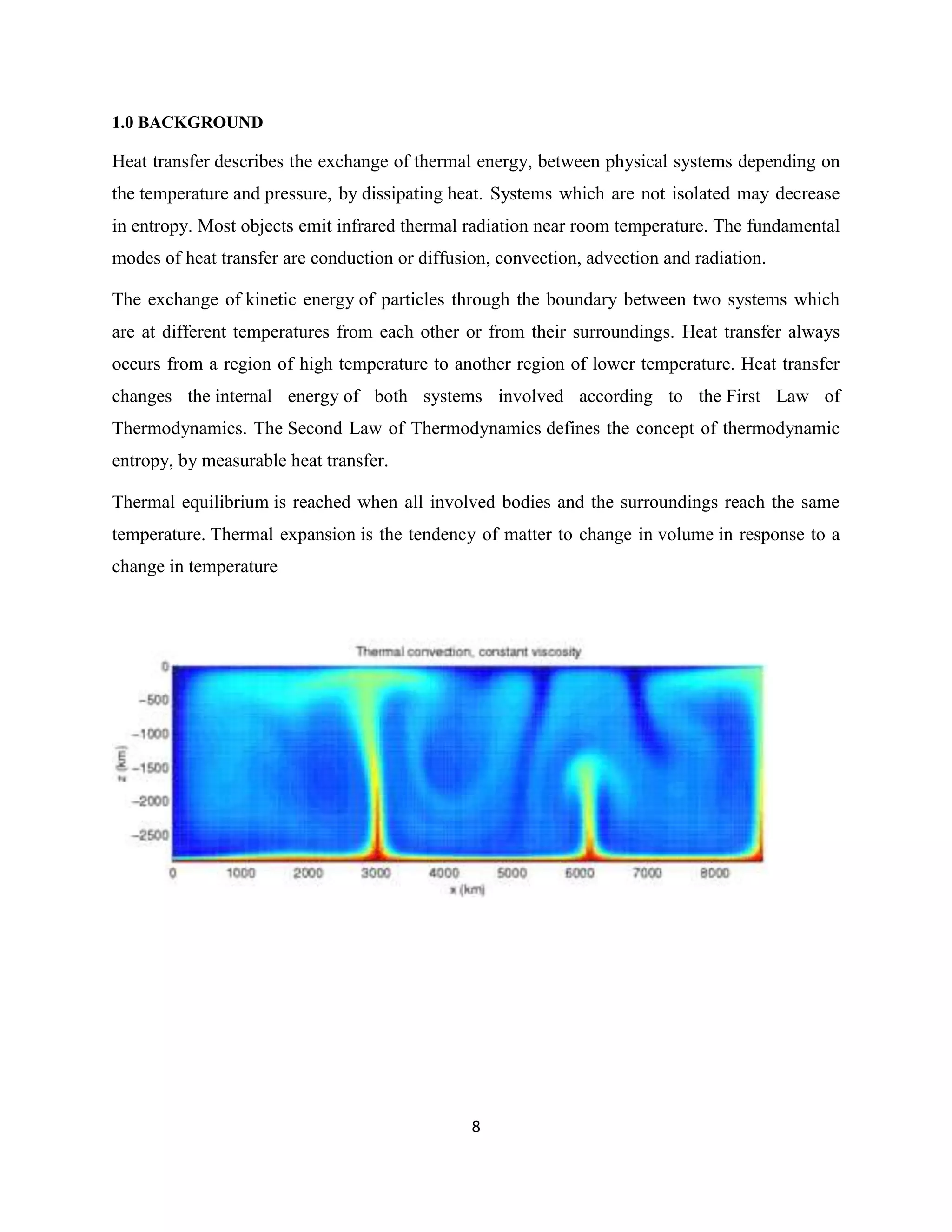
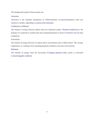
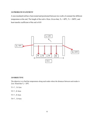
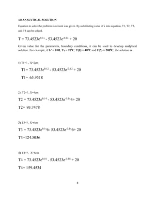
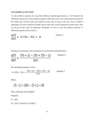
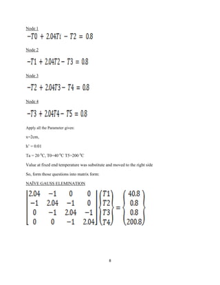
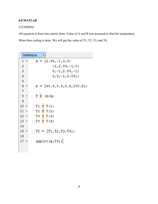
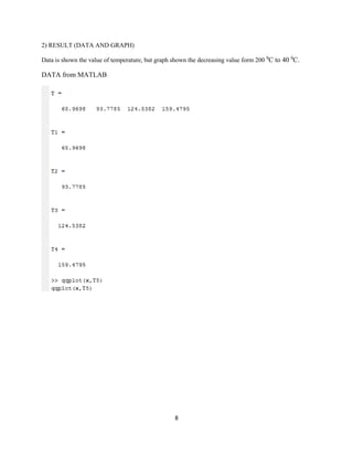
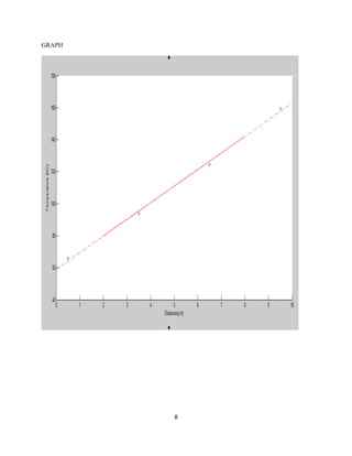
The document discusses heat transfer between systems at different temperatures. It provides background on the fundamental modes of heat transfer (conduction, convection, radiation, advection). It then presents a problem statement involving the temperature at different points along a rod with varying temperatures at its ends. Both analytical and numerical solutions are developed to calculate the temperatures at each point. The numerical solution uses a finite difference method and matrix equations in MATLAB to calculate temperatures with higher accuracy than the analytical solution.

1. 8
1.0 BACKGROUND
Heat transfer describes the exchange of thermal energy, between physical systems depending on
the temperature and pressure, by dissipating heat. Systems which are not isolated may decrease
in entropy. Most objects emit infrared thermal radiation near room temperature. The fundamental
modes of heat transfer are conduction or diffusion, convection, advection and radiation.
The exchange of kinetic energy of particles through the boundary between two systems which
are at different temperatures from each other or from their surroundings. Heat transfer always
occurs from a region of high temperature to another region of lower temperature. Heat transfer
changes the internal energy of both systems involved according to the First Law of
Thermodynamics. The Second Law of Thermodynamics defines the concept of thermodynamic
entropy, by measurable heat transfer.
Thermal equilibrium is reached when all involved bodies and the surroundings reach the same
temperature. Thermal expansion is the tendency of matter to change in volume in response to a
change in temperature

2. 8
The fundamental modes of heat transfer are:
Advection
Advection is the transport mechanism of a fluid substance or conserved property from one
location to another, depending on motion and momentum.
Conduction or diffusion
The transfer of energy between objects that are in physical contact. Thermal conductivity is the
property of a material to conduct heat and evaluated primarily in terms of Fourier's Law for heat
conduction.
Convection
The transfer of energy between an object and its environment, due to fluid motion. The average
temperature, is a reference for evaluating properties related to convective heat transfer.
Radiation
The transfer of energy from the movement of charged particles within atoms is converted
to electromagnetic radiation.

3. 8
2.0 PROBLEM STATEMENT
A non-insulated rod have been tested and positioned between two walls of constant but different
temperature at the end. The length of the rod is 10cm. Given that, T0 = 400C, T5 = 2000C, and
heat transfer coefficient of the rod is 0.01
3.0 OBJECTIVE
The objective is to find the temperatures along each nodes where the distances between each nodes is
2cm. Noted that Ta = 200C
T1=? , X=2cm
T2=? , X=4cm
T3=? , X=6cm
T4=? , X=8cm

4. 8
4.0 ANALYTICAL SOLUTION
Equation to solve the problem statement was given. By substituting value of x into equation, T1, T2, T3,
and T4 can be solved.
T = 73.4523e0.1x - 53.4523e-0.1x + 20
Given value for the parameters, boundary conditions, it can be used to develop analytical
solution. For example, if h’ = 0.01, Ta = 200C, T(0) = 400C and T(5) = 2000C, the solution is
1) T1=? , X=2cm
T1= 73.4523e0.12 - 53.4523e-0.12 + 20
T1= 65.9518
2) T2=? , X=4cm
T2 = 73.4523e0.14 - 53.4523e-0.1x4+ 20
T2= 93.7478
3) T3=? , X=6cm
T3 = 73.4523e0.1x6- 53.4523e-0.1x6+ 20
T3=124.5036
4) T4=? , X=8cm
T4 = 73.4523e0.18 - 53.4523e-0.18 + 20
T4= 159.4534

5. 8
5.0 NUMERICAL SOLUTION
To solve problem statement, by using finite difference method approximations, it will transform the
differential equation into a linear algebraic equations which then can be solve using numerical method for
this steady state. Find the steady state equation to each node. It mean, in this case I have 4 unknown
temperature. So I have 4 equation of steady state for each node. Form all equation into matrix form. Then
we will get all the value of temperature. Remember, no error to solve this problem statement. A
differential equation can be written as
Equation 1
Calculus was necessary to be use because it involved the second derivative.
Equation 2
By substituting equation 1 into 2,
Equation 3
Hence,
Thus, each node can be applied
Parameter:
h’ = 0.01
Ta = 20 0C, T0=40 0C T5=200 0C

6. 8
Node 1
Node 2
Node 3
Node 4
Apply all the Parameter given:
x=2cm,
h’ = 0.01
Ta = 20 0C, T0=40 0C T5=200 0C
Value at fixed end temperature was substitute and moved to the right side
So, form those questions into matrix form:
NAÏVE GAUSS ELEMINATION

7. 8
6.0 MATLAB
1) CODING
All equation is form into matrix form. Value of A and B was assumed to find the temperature.
When then coding is done. We will get the value of T1, T2, T3, and T4.

8. 8
2) RESULT (DATA AND GRAPH)
Data is shown the value of temperature, but graph shown the decreasing value form 200 0C to 40 0C.
DATA from MATLAB

9. 8
GRAPH

10. 8
7.0 DISCUSSION
By using the finite difference approximations, the temperature for the entire node can be easily calculated:
Which,
T1= 65.9698 0C, T2= 93.7785 0C, T3= 124.5382 0C,
T4= 159.4795 0C
Based on the graph, it can see the true value of the temperature along the distance between 0cm to 10 cm.
It knows by using numerical approximate is the best way to solve the problem in heat transfer. Simple
step of numerical solution is very useful to apply it. On the graph, it can see linear graph of the
temperature slowing down until T0. By using this method, it easy to find the true value along the distance
compared to the analytical solution. If using the analytical solution it needs to find the equation first and it
can solve the problem statement but it only can get the temperature at the node only. Example, it can see
how much reducing of temperature from 0cm to 5 cm in term of temperature base on linear graph but if
use analytical solution it cannot find the temperature at 5cm unless apply the equation and then repeat the
same steps. If compared analytical method between numerical methods to the value of temperature, it
showed the difference value. Example, at node 1, by using analytical solution, value of temperature T1 is
65.9518 compared to numerical method, value of temperature T1 is 65.9698. By using the numerical
method, it proved the value of the temperature more accurate compared to analytical method.

11. 8
8.0 CONCLUSION
Lastly, by using numerical method is the best way to solve heat transfer problem. It can get the true value
and more accurate value compared to analytical method. Numerical method is easier to apply it. In
numerical method, there are several types of method can be used to solve heat transfer problem. But by
using naive gauss elimination is easier to apply and to understand of this method.
9.0 REFERENCES
1) http://en.wikipedia.org/wiki/Numerical_analysis
2) http://en.wikipedia.org/wiki/Heat_transfer
3) http://hyperphysics.phy-astr.gsu.edu/hbase/thermo/heatra.html
4) http://www.efunda.com/formulae/heat_transfer/home/overview.cfm