field theory

1. Sweeping Discussions On Dirac Fields
Roa, F. J. P.
We write
(1)
tni
LL
ffe LLL ),()()( 2122  
as a Lagrangian for a basic electron theory that can be outlined from an SU(2)XU(1)
construction that excludes as yet the additional fermions needed in the full electroweak
theory. Lagrangian (1) includes an effective Lagrangian ffeL )( 2 for the electron 2
and an interaction Lagrangian tni
LL
L ),( 21  exclusive only for the lefthanded
(electron) neutrino L
1 , which is massless, and the lefthanded electron L
2 that has mass.
The effective Lagrangian (for the electron 2 ), aside from the free Lagrangian 02 )(L
present in it, also contains tniL )( 2 , which serves as an interaction Lagrangian in the
said effective lagrangian ( ffeL )( 2 ) that includes the interactions of the electron with
the Higgs boson , the electromagnetic field me
A that is massless, and one massive field
Z .
(2.1)
tniffe LLL )()()( 2022  
(2.2)
 
 LRR
RLL
mi
mi
miL
222
222
222202 )(












Let it be noted that all equations appearing in this document are in Heaviside units in
which 1 c and that the Dirac mass m is simply given in terms of the Yukawa
coupling constant y and the non-zero vacuum expectation value (vev)  of the Higgs
field,

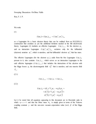
2. (2.3)
 ym 
(2.4)
  22222 tan)(  

ZeAeyL me
tni 
This Lagrangian can ofcourse be viewed in terms of the lefthanded electron and its
counter-part, R
2 .
(2.5.1)
  2
5
2 1
2
1
 L
(2.5.2)
  2
5
2 1
2
1
 R
(I must emphasize that in this document, our definitions for L
2 and R
2 are as given by
the preceding equations above.)
Given (2.5.1) and (2.5.2), the said effective Lagrangian can be decomposed under the
following expressions
(2.6.1)
222222   RLLR
(2.6.2)
222222  
 RRLL
(2.6.3)
222222  





 RRLL
For the interaction Lagrangian tni
LL
L ),( 21  , one thing to notice in this is that this
excludes the righthanded electron R
2 and represents the interactions of the massless
lefthanded neutrino L
1 and lefthanded electron L
2 with the weak gauge bosons.
(2.7)

3.  )(
12
)(
21
1
22
1
21
)sin2(
)cossin2(),(












WWe
ZeL
LLLL
LL
tni
LL
Let us take ffeL )( 2 from (1) and with it form the action
(3.1)
ffeffe LxdS )()( 2
4
2  
We may think of it as an effective electron theory that we can outline from a basic
SU(2)XU(1) construction without as yet the additional fermions of electroweak theory.
In the said action (3.1), we may proceed with the four integral contained in it
(3.2)
  







3
1
220
0
2
30
22
4
l
l
l
ixdxdixd  
 
From (3.2), say we perform the one integral over time ( tx 0
) first, assuming we are
given with two end-points ( 00
BA xandx ) in time and thus, by integration by-parts we
have
(3.3)
    2
0
20
0
)(
)(
2
0
220
0
2
0
)(
0
0
 ixdiixd
Bx
Ax
We can use this to write one four integral in (3.2) as
(3.4)
     2
0
20
4
)(
)(
2
0
2020
0
2
4
)(
0
0
 ixdidixd
Bx
Ax
where for example, 0
d is a short for
(3.5)
32130
dxdxdxxdd 


In the same way we can manipulate for any given space part in (3.2)
(3.6)

4.      22
4
)(
)(
2222
4
)(  l
l
Bx
Ax
l
ll
l
ixdidixd
l
l
Thus, by integration by-parts we are able to re-write (3.2) into a desired form
(3.7)
     22
4
)(
)(
2222
4
)(  



 

ixdidixd
Bx
Ax
Consequently, using (3.7) we may put (3.1) in the following form
(3.8.1)
     222222
4)(
)(222 )()(  




 q
Bx
Axffe FyixdidS
(3.8.2)




 ZeeAyF me
q tan
What we have done here in using integration by-parts (3.7) in (3.1) is a recasting of this
action, which is held as an effective action for the spinor field 2 , into an action
ffeS )( 2 for the adjoint spinor field 2 .
(3.9)
 



222222
4
2
4
2
)(
)()(



 q
ffeffe
Fyixd
LxdS
We may think of (3.1) and (3.9) as two separate theories that are adjoint to each other. In
these actions, we can take 2 and 2 as two independent spinor fields and we can obtain
the total simultaneous variations of these actions in terms of the variations of the cited
field variables.
From (3.1) we obtain the total variation
(3.10.1)
 
 
  2222
4
2222
4
)(
)(222
)(
)(

















q
q
Bx
Ax
Fyixd
Fyixd
idS

5. while from (3.9) we have
(3.10.2)
 
 
  2222
4
2222
4
)(
)(222
)(
)(

















q
q
Bx
Ax
Fyixd
Fyixd
idS
In the classical context, we can impose the boundary condition that the varied fields (
2 and 2 ) vanish at the two end-points A and B. Thus, rendering the effective
forms of (3.10.1) and (3.10.2) equivalent
(3.11)
ffeffe SS )()( 22  
To get Dirac’s first order equation of motion for the independent field 2 , we vary
action (3.1) with respect to the adjoint spinor 2 alone and this yields
(4.1)
)(
)(
2
2
2
2
2
2
2
2
4
22
)(
)()(
)/(
Bx
Ax
ffe
ffeffe
L
d
LL
xdS




































This, obtained by invoking the commutativity in
(4.2)
  
and after integration by-parts. Again, in the classical context we impose the spacetime
boundary condition on the varied field 2 to obtain the effective form of (4.1)

6. (4.3.1)
 









2
2
2
2
2
4
22
)()(
)/(







ffeffe
ffe
LL
xdS
(4.3.2)
0)()( 22  BA 
Also, in the classical context, we render this effective variation stationary
(4.4.1)
0)/( 22 ffeS 
we obtain the Euler-Lagrange equation
(4.4.2)
0
)()(
2
2
2
2









ffeffe LL
and upon noting that
(4.4.3)
0
)(
2
2

 


ffeL
and
(4.4.4)
222
2
2 )(





q
ffe
Fyi
L

we arrive at the said first order equation
(4.4.5)
0222   

qFyi

7. In the case for the adjoint spinor 𝜓̅2 as an independent field, its own equation of motion
can in one way obtained from the same action (3.1) although varying this with respect to
the spinor 𝜓2 alone while putting the said action in the given form
(5.1)
  )()( 2
)(
)(222  


 SidS
Bx
Ax  
where )( 2S is the independent action for the independent field 𝜓̅2 and is given by
(3.9).
The said variation of (5.1) in terms only of the variation 𝛿𝜓2 can be put in the form
(5.2.1)
  )/()/( 22
)(
)(2222  


 SidS
Bx
Ax  
Repeatedly, in the classical context, the varied field 𝛿𝜓2 must vanish at the two end
points in spacetime, rendering the effective variation of (5.1) equal to the variation of
(3.9) with respect to the field variable 𝜓2,
(5.2.2)
)/()/( 2222  SS ffe 
(5.2.3)
0)()( 22  BA 
With the vanishing of the varied field at the end points we can also reduce the right-hand-
side of (5.2.2) into its effective form.
In turn, we get the variation
(5.3.1)
)(
)(2
2
2
2
2
2
2
24
22
)(
)()(
)/(
Bx
Ax
ffe
ffeffe
L
d
LL
xdS







































8. and with the imposition of (5.2.3) this gets reduced to
(5.3.2)
2
2
2
2
24
22
)()(
)/( 






 









ffeffe LL
xdS
In the same way that we have treated variation (4.4.1), we also hold variation (5.3.2)
stationary
(5.3.3)
0)/( 22 ffeS 
and from it, obtaining the Euler-Lagrange equation for the adjoint spinor field 2
(5.3.4)
0
)()(
2
2
2
2









ffeffe LL
This leads to the first order equation for the adjoint spinor
(5.3.5)
0)( 222  qFyi  

upon noting that
(5.3.6)
0
)(
2
2

 


ffeL
and
(5.3.7)
q
ffe
Fyi
L
222
2
2
)(
)(


 
 

9. Let’s take first order equation (4.4.5) and write for it the wave solution which consists of
superposition of individual waves, each carrying a spatial wave number 𝑘⃗ . I’m used to
writing this solution in the following form
(6.1.1)
𝜓2 ( 𝑥) = 𝜓2( 𝑥, 𝑥0) =
1
√(2𝜋)3
∑ 𝜓̃2
𝑘⃗
(𝑘⃗ , 𝑥0
)𝑒 𝑖𝑘⃗ ∙𝑥
where each fourier component 𝜓̃2(𝑘⃗ , 𝑥0
) carries the spatial wave number 𝑘⃗ and
expressed as an inverse fourier transform over the continuous zeroth wave number
component 𝑘0
.
(6.1.2)
𝜓̃2(𝑘⃗ , 𝑥0
) =
1
√2𝜋
∫ 𝑑𝑘0
𝜓̃2(𝑘⃗ , 𝑘0
) 𝑒−𝑖𝑘0
𝑥0
Given the fourier component, we can also write the wave solution as
(6.1.3)
𝜓2 ( 𝑥) = 𝜓2 ( 𝑥, 𝑥0) =
1
(2𝜋)2
∑ ∫ 𝑑𝑘0
𝜓̃2
𝑘⃗
(𝑘⃗ , 𝑘0
)𝑒−𝑖𝑘 𝜆 𝑥 𝜆
with a metric signature of -2.
Note that (6.1.3) is in terms of discrete spatial wave number 𝑘⃗ and we can switch to the
continuous case by noting the equivalence
(6.1.4)
1
√(2𝜋)3
∑
𝑘⃗
=
1
√(2𝜋)3
∫ 𝑑3
𝑘⃗
while also noting, given the relation (𝑝 = ℏ𝑘⃗ ) between the spatial momentum 𝑝 and this
wave number 𝑘⃗ , we can also write
(6.1.5)
1
√ 𝑉
∑ =
1
√(2𝜋)3
∑
𝑘⃗𝑃⃗

10. It must be noted that the fourier components 𝜓̃2(𝑘⃗ , 𝑘0
) in (6.1.3) are themselves Dirac
spinors, 4 × 1 column matrices with complex components.
We would also write for the source 𝐹𝑞 in terms of its fourier components, identical in
form to that of (6.1.3).
Applying the fourier integral (6.1.3) along with the identical form of integral to be
defined for 𝐹𝑞, we would be able to re-express the cited first order equation (4.4.5) in
consequent fourier integral form also
(6.2)
1
(2𝜋)2
∫ 𝑑4
𝑘′ (𝛾 𝜇
𝑘′
𝜇 − 𝑦𝛽)𝜓̃2 (𝑘′
)𝑒−𝑖𝑘′
𝜎 𝑥 𝜎
=
1
(2𝜋)4
∫ 𝑑4
𝑘′′
𝑑4
𝑘′′′
𝐹̃𝑞( 𝑘′′′) 𝜓̃2(𝑘′′
) 𝑒−𝑖(𝑘′′
𝜎 + 𝑘′′′
𝜎 )𝑥 𝜎
To obtain the fourier components, we are to integrate both sides with
(6.3)
1
(2𝜋)2
∫ 𝑑4
𝑥 ⋯ 𝑒 𝑖𝑘 𝜎 𝑥 𝜎
and make use of the integral fourier representation of delta function
(6.4)
𝛿4( 𝑘 − 𝑘′) =
1
(2𝜋)4
∫ 𝑑4
𝑥 𝑒 𝑖(𝑘 𝜇− 𝑘′
𝜇 )𝑥 𝜇
Thus, from (6.2), we arrive at
(6.5.1)
(𝛾 𝜇
𝑘 𝜇 − 𝑦𝛽)𝜓̃2(𝑘) =
1
(2𝜋)2
∫ 𝑑4
𝑘′′
𝑑4
𝑘′′′
𝐹̃𝑞( 𝑘′′′) 𝜓̃2 (𝑘′′
) 𝛿4( 𝑘′′
+ 𝑘′′′
− 𝑘)
or express the fourier component 𝜓̃2( 𝑘) solution as
(6.5.2)
𝜓̃2( 𝑘) =
1
(2𝜋)2
∫ 𝑑4
𝑘′′
𝑑4
𝑘′′′
(𝛾 𝜇
𝑘 𝜇 − 𝑦𝛽)
− 1
𝐹̃𝑞( 𝑘′′′) 𝜓̃2( 𝑘′′) 𝛿4( 𝑘′′
+ 𝑘′′′
− 𝑘)

11. In (6.5.1), we identify the Dirac propagator as
(6.5.3)
𝐺̃ 𝜓(𝑘) = (𝛾 𝜇
𝑘 𝜇 − 𝑦𝛽)
− 1
=
𝛾 𝜐
𝑘 𝜐 + 𝑦𝛽
𝑘 𝜇 𝑘 𝜇 − (𝑦𝛽)2
Ref’s:
[1]W. Hollik, Quantum field theory and the Standard Model, arXiv:1012.3883v1 [hep-
ph]
[2]Baal, P., A COURSE IN FIELD THEORY,
http://www.lorentz.leidenuniv.nl/~vanbaal/FTcourse.html
[3]’t Hooft, G., THE CONCEPTUAL BASIS OF QUANTUM FIELD THEORY,
http://www.phys.uu.nl/~thooft/
[4]Siegel, W., FIELDS, arXiv:hep-th/9912205 v2
[5]Wells, J. D., Lectures on Higgs Boson Physics in the Standard Model and Beyond,
arXiv:0909.4541v1
[6]Cardy, J., Introduction to Quantum Field Theory
[7]Gaberdiel, M., Gehrmann-De Ridder, A., Quantum Field Theory