SlideShare a Scribd company logo
1 of 10
Download to read offline
A simple finite element solver for thermo-mechanical problems
Keywords: Scilab, Open source software, thermo-elasticity
Introduction
In this paper we would like to show how it is possible to develop a simple but effective finite
element solver to deal with thermo-mechanical problems. In many engineering situations it is
necessary to solve heat conduction problems, both steady and unsteady state, to estimate the
temperature field inside a medium and, at the same time, compute the induced strain and stress
states.
To solve such problems many commercial software tools are available. They provide user-friendly
interfaces and flexible solvers, which can also take into account very complicated boundary
conditions, such as radiation, and nonlinearities of any kind, to allow the user to model the reality in
a very accurate and reliable way.
However, there are some situations in which the problem to be solved requires a simple and
standard modeling: in these cases it could be sufficient to have a light and dedicated software able
to give reliable solutions. Moreover, other two desirable features of such a software could be the
possibility to access the source to easily program new tools and, last but not least, to have a cost-
and-license free product. This turns out to be very useful when dealing with the solution of
optimization problems.
Keeping in mind these considerations, we used the Scilab platform and the gmsh (which are both
open source codes: see [1] and [2]) to show that it is possible to build tailored software tools, able to
solve standard but complex problems quite efficiently.
Feature Commercial codes In-house codes
Flexibility
It strongly depends on the code.
Commercial codes are thought to be
general purpose but rarely they can be
easily customized.
In principle the maximum flexibility
can be reached with a good
organization of programming.
Applications tailored on a specific
need can be done.
Cost
The license cost strongly depends on the
code. Sometimes a maintenance has to
be paid to access updates and upgrades.
No license means no costs, except
those coming out from the
development.
Numerics and
mathematics
knowledge required
No special skills are required even if an
intelligent use of simulation software
requires a certain engineering or
scientific background.
A certain background in mathematics,
physics and numerical techniques is
obviously necessary.
Programming skills Usually no skills are necessary.
It depends on the language and
platform used and also on the
objectives that lead the development.
Performance
Commercial codes use the state-of –the-
art of the high performance computing
to provide to the user very efficient
applications.
The performance strongly depends on
the way the code has been written.
Reliability of results
Usually commercial codes do not
provide any warranty on the goodness of
results, even though many benchmarks
are given to demonstrate the
effectiveness of the code.
A benchmarking activity is
recommended to debug in-house
codes and to check the goodness of
results. This could take a long time.
Table 1: A simple comparison between commercial and in-house software is made in this table. These
considerations reflect the author opinion and therefore the reader could not agree. The discussion is open.
Of course, to do this it is necessary to have a good knowledge basis in finite element formulations
but no special skills in programming, thanks to the ease in developing code which characterizes
Scilab.
In this paper we firstly discuss about the numerical solution of the parabolic partial differential
equation which governs the unsteady state heat transfer problem and then a similar strategy for the
solution of elastostatic problems will be presented. These descriptions are absolutely general and
they represent the starting point for more complex and richer models. The main objective of this
work is certainly not to present revolutionary results or new super codes, but just and simply to
show that in some cases it could be feasible, useful and profitable to develop home-made
applications.
The thermal solver
The first step to deal with is to implement a numerical technique to solve the unsteady state heat
transfer problem described by the following partial differential equation:
ߩܿ
డ்
డ௧
െ ‫׏‬ · ሺ݇‫ܶ׏‬ሻ ൌ ݂ ݅݊ Ω (1)
which has to be solved in the domain Ω, taking into account the boundary conditions, which apply
on different portions of the boundary (Γ ൌ Γ୘ ‫ڂ‬ Γ୕ ‫ڂ‬ Γେ). They could be of Dirichlet, Neumann or
Robin kind, expressing a given temperature ܶത, a given flux ܳത or a convection condition with the
environment:
ܶ ൌ ܶത ‫݊݋‬ Γ୘
െ݇
డ்
డ࢔ෝ
ൌ ܳത ‫݊݋‬ Γ୕
െ݇
డ்
డ࢔ෝ
ൌ ݄ሺܶ െ ܶതாሻ ‫݊݋‬ Γେ
(2)
being ࢔ෝ the unit normal vector to the boundary and the upper-lined quantities known values at each
time. The symbols “‫׏‬ ·” and “‫”׏‬ are used to indicate the divergence and the gradient operator
respectively, while ܶ is the unknown temperature field. The medium properties are the density ߩ,
the specific heat ܿ and the thermal conductivity ݇ which could depend, in a general case, on
temperature. The term ݂ on the right hand side represents all the body sources of heat and it could
depend on both the space and time.
For sake of simplicity we imagine that all the medium properties are constant; in this way the
problem comes out to be linear, dramatically simplifying the solution.
For the solution of the equations reported in (1) we decide to use a traditional Galerkin residual
approach. To this aim, it is necessary to introduce a virtual field ܶ෨ and consider the weighted
version of equation (1):
‫׬‬ ܶ෨ ቀߩܿ
డ்
డ௧
െ ‫׏‬ · ሺ݇‫ܶ׏‬ሻ െ ݂ቁΩ
݀Ω (3)
The divergence theorem can be invoked to rewrite this equation in a more treatable way. Actually,
we have:
‫׬‬ ܶ෨‫׏‬ · ݇‫ܶ׏‬Ω
݀Ω ൌ ‫׬‬ ܶ෨݇‫ܶ׏‬ · ࢔ෝ݀Γ െ ‫׬‬ ‫ܶ׏‬෨݇‫ܶ׏‬Ω
݀Ω୻
(4)
The integral over Γ involves the boundary flux. Equation (3) can be rewritten as:
‫׬‬ ܶ෨ߩܿ
డ்
డ௧
݀Ω ൅ ‫׬‬ ܶ෨‫׏‬ · ሺ݇‫ܶ׏‬ሻ݀ΩΩ
ൌ ‫׬‬ ܶ෨݂ΩΩ
݀Ω ൅ ‫׬‬ ܶ෨݇‫ܶ׏‬ · ࢔ෝdΓ୻
(5)
In order to solve numerically the above equation it is necessary to introduce a discretization of the
domain Ω and choose appropriate test functions.
Equations (5) can be rewritten, once the discretization has been introduced, as the appropriate sum
over the elements of certain contributions that can be computed numerically by means of a standard
Gauss integration. The We obtain, in matrix form, the following expression:
ሾ‫ܥ‬ሿሼܶሽሶ ൅ ሾ‫ܭ‬ሿሼܶሽ ൌ ሼ‫ܨ‬ሽ (6)
where the symbols ሾ·ሿ and ሼ·ሽ are used to indicate matrices and vectors.
A classical Euler scheme can be implemented. If we assume the following approximation for the
first time derivative of the temperature field:
ߴ൛ܶሶ௡ାଵൟ ൅ ሺ1 െ ߴሻ൛ܶሶ௡ൟ ൌ
ሼ்೙శభሽିሼ்೙ሽ
୼௧
(7)
being ߴ ൌ ሾ0,1ሿ and Δܶ the time step, we can rewrite, after some manipulation, equation (6) as:
ቀ
ሾ஼ሿ
୼்
൅ ߴሾ‫ܭ‬ሿቁ ሼܶ௡ାଵሽ െ ቀ
ሾ஼ሿ
୼்
൅ ሺߴ െ 1ሻሾ‫ܭ‬ሿቁ ሼܶ௡ሽ ൌ ߴሼ‫ܨ‬௡ାଵሽ ൅ ሺ1 െ ߴሻሼ‫ܨ‬௡ሽ (8)
It is well known (see [4]) that the value of the parameter ߴ plays a fundamental role. If we choose
ߴ ൌ 0 an explicit time integration scheme is obtained, actually the unknown temperature at step
n+1 can be explicitly computed starting from already computed or known quantities.
Moreover, the use of a lumped finite element approach leads to a diagonal matrix ሾ‫ܥ‬ሿ; this is a
desirable feature, because the solution of equation (8), which passes through the inversion of ሾ‫ܥ‬ሿ,
reduces to simple and fast computations. The gain is much more evident if a non-linear problem has
to be solved, when the inversion of ሾ‫ܥ‬ሿ has to be performed at each integration step.
Unfortunately, this scheme is not unconditionally stable; the time integration step Δ‫ݐ‬ has actually to
be less than a threshold which depend on the nature of the problem and on the mesh. In some cases
this restriction could require very small time steps, giving high solution time.
On the contrary, if ߴ ൌ 1, an implicit scheme comes out from (8), which can be specialized as:
ቀ
ሾ஼ሿ
୼்
൅ ሾ‫ܭ‬ሿቁ ሼܶ௡ାଵሽ െ
ሾ஼ሿ
୼்
ሼܶ௡ሽ ൌ ߴሼ‫ܨ‬௡ାଵሽ (9)
In this case the matrix on the left involves also the conductivity contribution, which cannot be
diagonalized trough a lumped approach and therefore the solution of a system of linear equations
has to be computed at each step. The system matrix is however symmetric and positive definite, so
a Choleski decomposition can be computed once for all and at each integration step the backward
process, which is the less expensive from a computational point of view, can be performed.
This scheme has the great advantage to be unconditionally stable: this means that there are no
restriction on the time step to adopt. Obviously, the larger the step, the larger the errors due to the
time discretization introduced in the model, according to (7).
In principle all the intermediate values for ߴ are possible, considering that the stability of the Euler
scheme is guaranteed for ߴ ൐ 1 2⁄ , but usually the most used version are the full explicit or implicit
one.
In order to test the goodness of our application we have performed many tests and comparisons.
Here we present the simple example depicted in Figure 1. Let us imagine that in a long circular pipe
a fluid flows with a temperature which changes with time according to the law drawn in Figure 1,
on the right. We want to estimate the temperature distribution at different time steps inside the
medium and compute the temperature in the point P.
It is interesting to note that for this simple problem all the boundary conditions described in (2)
have to be used. A unit density and specific heat for the medium has been taken, while a thermal
conductivity of 5 has been chosen for this benchmark. The environmental temperature has been set
to 0 and the convection coefficient to 5.
As shown in the following pictures there is a good agreement between the results obtained with
Ansys Workbench and our solver.
Figure 1: In view of the symmetry of the pipe problem we can consider just one half of the structure during the
computations. A null normal flux on the symmetry boundary has been applied to model symmetry as on the base
line (green boundaries), while a convection condition has been imposed on the external boundaries (blue
boundaries). Inside the hole a temperature is given according to the law described on the right.
Figure 2: Temperature field at time 30 The Ansys Workbench (left) and our solver (right) results. A good
agreement can be seen comparing these two images.
Figure 3: Temperature field in the point P plotted versus time. The Ansys Workbench (red) and our solver (blue)
results. Also in this case a good agreement between results is achieved.
The structural solver
If we want to solve a thermo-structural problem (see [3] and references reported therein) we
obviously need a solver able to deal with the elasticity equations. We focus on the simplest case,
that is two dimensional problems (plane strain, plane stress and axi-symmetric problems) with a
completely linear, elastic and isotropic response. We have to take into account that a temperature
field induces thermal deformations inside a solid medium. Actually:
ߝ௜௜
்ு
ൌ ߙሺܶ െ ܶோாிሻ (10)
where the double index i indicates that no shear deformation can appear. The ܶோாி represents the
reference temperature at which no deformation is produced inside the medium.
Once the temperature field is known at each time step, it is possible to compute the induced
deformations and then the stress state.
For sake of simplicity we imagine that the loads acting on the structure are not able to produce
dynamic effects and therefore, if we neglect the body forces contributions, the equilibrium equations
reduce to:
‫׏‬ · ࣌ ൌ 0 or, with the indicial notation
డఙ೔ೕ
డ௫ೕ
ൌ 0 (11)
The elastic deformation ࢿ can be computed as the difference between the total and the thermal
contributions as:
ࢿ ൌ ࢿ்ை்
െ ࢿ்ு
(12)
which can be expressed in terms of the displacement vector field ࢛ as:
ࢿ ൌ
ଵ
ଶ
ሺ‫࢛׏‬ ൅ ‫׏‬୲
࢛ሻ or, with the indicial notation ߝ௜௝ ൌ
ଵ
ଶ
൬
డ௨ೕ
డ௫೔
െ
డ௨೔
డ௫ೕ
൰ (13)
A linear constitutive law for the medium can be adopted and written as:
࣌ ൌ ࡰࢿ (14)
where the matrix ࡰ will be expressed in terms of ߤ and ߣ which describe the elastic response of the
medium. Finally, after some manipulation involving equations (11), (13) and (14), one can obtain
the following governing equation, which is expressed in terms of the displacements field ࢛ only:
ሺߣ ൅ ߤሻ‫׏‬ሺ‫׏‬ · ࢛ሻ ൅ ߤ‫׏‬ଶ
࢛ െ ߙሺ3ߣ ൅ 2ߤሻ‫ܶ׏‬ ൌ 0 (15)
As usual, the above equation has to be solved together with the boundary conditions, which
typically are of Dirichlet (imposed displacements ࢛ഥ on Γ୳) or Neumann kind (imposed tractions ࢖ഥ
on Γ୮):
࢛ ൌ ࢛ഥ ‫݊݋‬ Γ୳
࣌ · ࢔ෝ ൌ ࢖ഥ ‫݊݋‬ Γ୮
(16)
The same approach described above for the heat transfer equation, the Galerkin weighted residuals,
can be used with equation (15) and a discretization of the domain can be introduced to numerically
solve the problem.
Obviously, we do not need a time integration technique anymore, being the problem a static one.
We will obtain a system of linear equations characterized by a symmetric and positive definite
matrix: special techniques can be exploited to take advantage of these properties in order to reduce
the storage requirements (e.g. a sparse symmetric storage scheme) and to improve the efficiency
(e.g. a Choleski decomposition, if a direct solver is adopted).
As for the case of the thermal solver, many tests have been performed to check the accuracy of the
results. Here we propose a classical benchmark involving a plate of unit thickness under tension
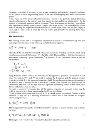
with a hole, as shown in Figure 4. A unit Young modulus and a Poisson coefficient of 0.3 have been
adopted to model the material behavior. The vertical displacements computed with Ansys and our
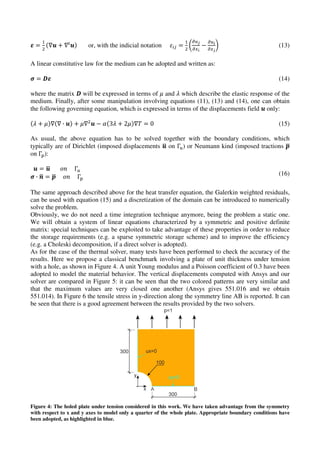
solver are compared in Figure 5: it can be seen that the two colored patterns are very similar and
that the maximum values are very closed one another (Ansys gives 551.016 and we obtain
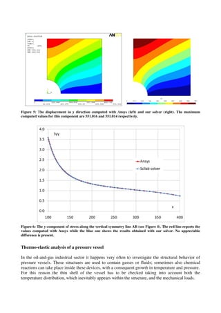
551.014). In Figure 6 the tensile stress in y-direction along the symmetry line AB is reported. It can
be seen that there is a good agreement between the results provided by the two solvers.
Figure 4: The holed plate under tension considered in this work. We have taken advantage from the symmetry
with respect to x and y axes to model only a quarter of the whole plate. Appropriate boundary conditions have
been adopted, as highlighted in blue.
Figure 5: The displacement in y direction computed with Ansys (left) and our solver (right). The maximum
computed values for this component are 551.016 and 551.014 respectively.
Figure 6: The y-component of stress along the vertical symmetry line AB (see Figure 4). The red line reports the
values computed with Ansys while the blue one shows the results obtained with our solver. No appreciable
difference is present.
Thermo-elastic analysis of a pressure vessel
In the oil-and-gas industrial sector it happens very often to investigate the structural behavior of
pressure vessels. These structures are used to contain gasses or fluids; sometimes also chemical
reactions can take place inside these devices, with a consequent growth in temperature and pressure.
For this reason the thin shell of the vessel has to be checked taking into account both the
temperature distribution, which inevitably appears within the structure, and the mechanical loads.
Figure 7: A simple sketch illustrates the vessel considered in this work. The revolution axis is drawn with the red
dashed line and some dimensioning (in [m]) is reported. The nozzle on top is closed thanks to a cap which is
considered completely bonded to the structure. The nozzle neck is not covered by the insulating material. On the
right the fluid temperature versus time is plotted. A pressure of 1 [MPa] acts inside the vessel.
Material
Density
[kg/m3
]
Specific heat
[J/kg°C]
Thermal
conductivity
[W/m°C]
Young
modulus
[N/m2
]
Poisson
ratio
[---]
Thermal expansion
coeff.
[1/°C]
Steel 7850 434 60.5 2.0·1011
0.30 1.2·10-5
Insulation 937 303 0.5 1.1·109
0.45 2.0·10-4
Table 2: The thermal and the mechanical properties of the materials involved in the analysis.
If we neglect the holes and the nozzles which could be present, the geometry of these structures can
be viewed, very often, as a solid of revolution. Moreover, the applied loads and the boundary
conditions reflect this symmetry and therefore it is very common, when applicable, to calculate a
vessel using an axi-symmetric approach.
In the followings we propose a thermo-mechanical analysis of the vessel depicted in Figure 7. The
fluid inside the vessel has a temperature which follows a two steps law (see Figure 7, on the right)
and a constant pressure of 1 [MPa]. We would like to know which is the temperature reached on the
external surface and which is the maximum stress inside the shell, with particular attention to the
upper neck.
We imagine that the vessel is made of a common steel and that it has an external thermal insulating
cover: the relevant material properties are collected in Table 2.
When dealing with a thermo-mechanical problem it could be reasonable to use two different meshes
to model and solve the heat transfer and the elasticity equations. Actually, if in the first case we
usually are interested in accurate modeling the temperature gradients, in the second case we would
like to have a reliable estimation of stress peaks, which in principle could appear in different zones
of the domain. For this reason we decided to have the possibility to use different computational
grids: once the temperature field is known, it will be mapped on to the structural mesh allowing in
this way a better flexibility of our solver.
In the case of the pressure vessel we decided to use a uniform mesh within the domain for the
thermal solver, while we adopted a finer mesh near the neck for the stress computation.
In Figure 8 the temperature field at time 150 [s] is drawn: on the right a detail of the neck is plotted.
It can be seen that the insulating material plays an important role, the surface temperature is actually
maintained very low. As mentioned above a uniform mesh is employed in this case.
Figure 8: The temperature field at time 150 [s] on the left and a detail of the neck on the right, where also the
mesh used for the solution of the thermal problem has been superimposed.
Figure 9: The radial (left) and vertical (right) displacement of the vessel.
Figure 10: The von Mises stress and a detail of the neck, on the right, together with the structural mesh.
In Figure 9 the radial (left) and the vertical (right) deformed shapes are plotted. In Figure 10 the von
Mises stress is drawn and , on the right, a detail in proximity of the neck is proposed: it can be
easily seen that the mesh has been refined in order to better capture the stress peaks in this zone of
the vessel.
Conclusions
In this work it has been shown how it is possible to use Scilab to solve thermo-mechanical
problems. For sake of simplicity the focus has been posed on two dimensional problems but the
reader has to remember that the extension to 3D problems does not require any additional effort
from a conceptual point of view.
Some simple benchmarks have been proposed to show the effectiveness of the solver written in
Scilab. The reader should have appreciated the fact that also industrial-like problems can be solved
efficiently, as the complete thermo-mechanical analysis of a pressure vessel proposed at the end of
the paper.
References
[1] http://www.scilab.org/ to have more information on Scilab
[2] The Gmsh can be freely downloaded from: http://www.geuz.org/gmsh/
[3] O. C Zienkiewicz, R. L. Taylor, The Finite Element Method: Basic Concepts and Linear
Applications (1989) McGraw Hill.
[4] M. R. Gosz, Finite Element Method. Applications in Solids, Structures and Heat Transfer
(2006) Francis &Taylor.
[5] Y. W. Kwon, H. Bang, The Finite Element Method using Matlab, (2006) CRC, 2nd
edition
Contacts
For more information on this document please contact the author:
Massimiliano Margonari
Enginsoft S.p.A.
m.margonari@enginsoft.it

More Related Content

What's hot

Adaptive response surface by kriging using pilot points for structural reliab...
Adaptive response surface by kriging using pilot points for structural reliab...Adaptive response surface by kriging using pilot points for structural reliab...
Adaptive response surface by kriging using pilot points for structural reliab...IOSR Journals
 
Parameter Estimation User Guide
Parameter Estimation User GuideParameter Estimation User Guide
Parameter Estimation User GuideAndy Salmon
 
Hybrid Simulated Annealing and Nelder-Mead Algorithm for Solving Large-Scale ...
Hybrid Simulated Annealing and Nelder-Mead Algorithm for Solving Large-Scale ...Hybrid Simulated Annealing and Nelder-Mead Algorithm for Solving Large-Scale ...
Hybrid Simulated Annealing and Nelder-Mead Algorithm for Solving Large-Scale ...IJORCS
 
An Elementary Introduction to Kalman Filtering
An Elementary Introduction to Kalman FilteringAn Elementary Introduction to Kalman Filtering
An Elementary Introduction to Kalman FilteringAshish Sharma
 
080924 Measurement System Analysis Re Sampling
080924 Measurement System Analysis Re Sampling080924 Measurement System Analysis Re Sampling
080924 Measurement System Analysis Re Samplingrwmill9716
 
Forecasting warranty returns with Wiebull Fit
Forecasting warranty returns with Wiebull FitForecasting warranty returns with Wiebull Fit
Forecasting warranty returns with Wiebull FitTonda MacLeod
 
Cpk guide 0211_tech1
Cpk guide 0211_tech1Cpk guide 0211_tech1
Cpk guide 0211_tech1Piyush Bose
 
An Update on my Gas Modelling Tools: Addition of New Shale Diagnostics, Gas S...
An Update on my Gas Modelling Tools: Addition of New Shale Diagnostics, Gas S...An Update on my Gas Modelling Tools: Addition of New Shale Diagnostics, Gas S...
An Update on my Gas Modelling Tools: Addition of New Shale Diagnostics, Gas S...Colin Jordan
 
MAST30013 Techniques in Operations Research
MAST30013 Techniques in Operations ResearchMAST30013 Techniques in Operations Research
MAST30013 Techniques in Operations ResearchLachlan Russell
 
Receptor kinetics Laplace transform method PDF
Receptor kinetics Laplace transform method PDFReceptor kinetics Laplace transform method PDF
Receptor kinetics Laplace transform method PDFSam Hoare
 
Receptor kinetics Laplace transform method Word
Receptor kinetics Laplace transform method WordReceptor kinetics Laplace transform method Word
Receptor kinetics Laplace transform method WordSam Hoare
 
Javier Garcia - Verdugo Sanchez - Six Sigma Training - W4 Monte Carlo Simulat...
Javier Garcia - Verdugo Sanchez - Six Sigma Training - W4 Monte Carlo Simulat...Javier Garcia - Verdugo Sanchez - Six Sigma Training - W4 Monte Carlo Simulat...
Javier Garcia - Verdugo Sanchez - Six Sigma Training - W4 Monte Carlo Simulat...J. García - Verdugo
 

What's hot (17)

Jg3616071610
Jg3616071610Jg3616071610
Jg3616071610
 
Adaptive response surface by kriging using pilot points for structural reliab...
Adaptive response surface by kriging using pilot points for structural reliab...Adaptive response surface by kriging using pilot points for structural reliab...
Adaptive response surface by kriging using pilot points for structural reliab...
 
Parameter Estimation User Guide
Parameter Estimation User GuideParameter Estimation User Guide
Parameter Estimation User Guide
 
Final Report 4_22_15
Final Report 4_22_15Final Report 4_22_15
Final Report 4_22_15
 
Hybrid Simulated Annealing and Nelder-Mead Algorithm for Solving Large-Scale ...
Hybrid Simulated Annealing and Nelder-Mead Algorithm for Solving Large-Scale ...Hybrid Simulated Annealing and Nelder-Mead Algorithm for Solving Large-Scale ...
Hybrid Simulated Annealing and Nelder-Mead Algorithm for Solving Large-Scale ...
 
An Elementary Introduction to Kalman Filtering
An Elementary Introduction to Kalman FilteringAn Elementary Introduction to Kalman Filtering
An Elementary Introduction to Kalman Filtering
 
Aws100 ch06 thermal
Aws100 ch06 thermalAws100 ch06 thermal
Aws100 ch06 thermal
 
Aws90 ch06 thermal
Aws90 ch06 thermalAws90 ch06 thermal
Aws90 ch06 thermal
 
080924 Measurement System Analysis Re Sampling
080924 Measurement System Analysis Re Sampling080924 Measurement System Analysis Re Sampling
080924 Measurement System Analysis Re Sampling
 
Forecasting warranty returns with Wiebull Fit
Forecasting warranty returns with Wiebull FitForecasting warranty returns with Wiebull Fit
Forecasting warranty returns with Wiebull Fit
 
Cpk guide 0211_tech1
Cpk guide 0211_tech1Cpk guide 0211_tech1
Cpk guide 0211_tech1
 
An Update on my Gas Modelling Tools: Addition of New Shale Diagnostics, Gas S...
An Update on my Gas Modelling Tools: Addition of New Shale Diagnostics, Gas S...An Update on my Gas Modelling Tools: Addition of New Shale Diagnostics, Gas S...
An Update on my Gas Modelling Tools: Addition of New Shale Diagnostics, Gas S...
 
MAST30013 Techniques in Operations Research
MAST30013 Techniques in Operations ResearchMAST30013 Techniques in Operations Research
MAST30013 Techniques in Operations Research
 
Receptor kinetics Laplace transform method PDF
Receptor kinetics Laplace transform method PDFReceptor kinetics Laplace transform method PDF
Receptor kinetics Laplace transform method PDF
 
Receptor kinetics Laplace transform method Word
Receptor kinetics Laplace transform method WordReceptor kinetics Laplace transform method Word
Receptor kinetics Laplace transform method Word
 
An introduction to weibull analysis
An introduction to weibull analysisAn introduction to weibull analysis
An introduction to weibull analysis
 
Javier Garcia - Verdugo Sanchez - Six Sigma Training - W4 Monte Carlo Simulat...
Javier Garcia - Verdugo Sanchez - Six Sigma Training - W4 Monte Carlo Simulat...Javier Garcia - Verdugo Sanchez - Six Sigma Training - W4 Monte Carlo Simulat...
Javier Garcia - Verdugo Sanchez - Six Sigma Training - W4 Monte Carlo Simulat...
 

Viewers also liked

Introduction to Discrete Probabilities with Scilab - Michaël Baudin, Consort...
Introduction to Discrete Probabilities with Scilab - Michaël Baudin, Consort...Introduction to Discrete Probabilities with Scilab - Michaël Baudin, Consort...
Introduction to Discrete Probabilities with Scilab - Michaël Baudin, Consort...Scilab
 
Scilab/Xcos pour l'enseignement des sciences de l'ingénieur
Scilab/Xcos pour l'enseignement des sciences de l'ingénieurScilab/Xcos pour l'enseignement des sciences de l'ingénieur
Scilab/Xcos pour l'enseignement des sciences de l'ingénieurScilab
 
Scilab Finite element solver for stationary and incompressible navier-stokes ...
Scilab Finite element solver for stationary and incompressible navier-stokes ...Scilab Finite element solver for stationary and incompressible navier-stokes ...
Scilab Finite element solver for stationary and incompressible navier-stokes ...Scilab
 
Scilab pour l'enseignement des mathématiques
Scilab pour l'enseignement des mathématiquesScilab pour l'enseignement des mathématiques
Scilab pour l'enseignement des mathématiquesScilab
 
Scilab debutant
Scilab debutantScilab debutant
Scilab debutantScilab
 
Xcos pour débutants
Xcos pour débutantsXcos pour débutants
Xcos pour débutantsScilab
 
ScilabTEC 2015 - Bavarian Center for Agriculture
ScilabTEC 2015 - Bavarian Center for AgricultureScilabTEC 2015 - Bavarian Center for Agriculture
ScilabTEC 2015 - Bavarian Center for AgricultureScilab
 
Xcos for beginners
Xcos for beginnersXcos for beginners
Xcos for beginnersScilab
 
Hydraulic Scilab toolbox for water distribution systems
Hydraulic Scilab toolbox for water distribution systemsHydraulic Scilab toolbox for water distribution systems
Hydraulic Scilab toolbox for water distribution systemsScilab
 
Scilab is not naive
Scilab is not naiveScilab is not naive
Scilab is not naiveScilab
 
Aeraulic toolbox for Xcos
Aeraulic toolbox for XcosAeraulic toolbox for Xcos
Aeraulic toolbox for XcosScilab
 
Scilab/Xcos pour l'enseignement des sciences de l'ingénieur
Scilab/Xcos pour l'enseignement des sciences de l'ingénieurScilab/Xcos pour l'enseignement des sciences de l'ingénieur
Scilab/Xcos pour l'enseignement des sciences de l'ingénieurScilab
 
Optimization in scilab
Optimization in scilabOptimization in scilab
Optimization in scilabScilab
 
Customizing Xcos with new Blocks and Palette
Customizing Xcos with new Blocks and PaletteCustomizing Xcos with new Blocks and Palette
Customizing Xcos with new Blocks and PaletteScilab
 

Viewers also liked (14)

Introduction to Discrete Probabilities with Scilab - Michaël Baudin, Consort...
Introduction to Discrete Probabilities with Scilab - Michaël Baudin, Consort...Introduction to Discrete Probabilities with Scilab - Michaël Baudin, Consort...
Introduction to Discrete Probabilities with Scilab - Michaël Baudin, Consort...
 
Scilab/Xcos pour l'enseignement des sciences de l'ingénieur
Scilab/Xcos pour l'enseignement des sciences de l'ingénieurScilab/Xcos pour l'enseignement des sciences de l'ingénieur
Scilab/Xcos pour l'enseignement des sciences de l'ingénieur
 
Scilab Finite element solver for stationary and incompressible navier-stokes ...
Scilab Finite element solver for stationary and incompressible navier-stokes ...Scilab Finite element solver for stationary and incompressible navier-stokes ...
Scilab Finite element solver for stationary and incompressible navier-stokes ...
 
Scilab pour l'enseignement des mathématiques
Scilab pour l'enseignement des mathématiquesScilab pour l'enseignement des mathématiques
Scilab pour l'enseignement des mathématiques
 
Scilab debutant
Scilab debutantScilab debutant
Scilab debutant
 
Xcos pour débutants
Xcos pour débutantsXcos pour débutants
Xcos pour débutants
 
ScilabTEC 2015 - Bavarian Center for Agriculture
ScilabTEC 2015 - Bavarian Center for AgricultureScilabTEC 2015 - Bavarian Center for Agriculture
ScilabTEC 2015 - Bavarian Center for Agriculture
 
Xcos for beginners
Xcos for beginnersXcos for beginners
Xcos for beginners
 
Hydraulic Scilab toolbox for water distribution systems
Hydraulic Scilab toolbox for water distribution systemsHydraulic Scilab toolbox for water distribution systems
Hydraulic Scilab toolbox for water distribution systems
 
Scilab is not naive
Scilab is not naiveScilab is not naive
Scilab is not naive
 
Aeraulic toolbox for Xcos
Aeraulic toolbox for XcosAeraulic toolbox for Xcos
Aeraulic toolbox for Xcos
 
Scilab/Xcos pour l'enseignement des sciences de l'ingénieur
Scilab/Xcos pour l'enseignement des sciences de l'ingénieurScilab/Xcos pour l'enseignement des sciences de l'ingénieur
Scilab/Xcos pour l'enseignement des sciences de l'ingénieur
 
Optimization in scilab
Optimization in scilabOptimization in scilab
Optimization in scilab
 
Customizing Xcos with new Blocks and Palette
Customizing Xcos with new Blocks and PaletteCustomizing Xcos with new Blocks and Palette
Customizing Xcos with new Blocks and Palette
 

Similar to A simple finite element solver for thermo-mechanical problems - margonari enginsoft

Steady state CFD analysis of C-D nozzle
Steady state CFD analysis of C-D nozzle Steady state CFD analysis of C-D nozzle
Steady state CFD analysis of C-D nozzle Vishnu R
 
Product failure analysis using Explicit dynamic
Product failure analysis using Explicit dynamicProduct failure analysis using Explicit dynamic
Product failure analysis using Explicit dynamicnaga ram
 
An Efficient Tangent Scheme For Solving Phase-Change Problems
An Efficient Tangent Scheme For Solving Phase-Change ProblemsAn Efficient Tangent Scheme For Solving Phase-Change Problems
An Efficient Tangent Scheme For Solving Phase-Change ProblemsDarian Pruitt
 
Computational Fluid Dynamics (CFD)
Computational Fluid Dynamics (CFD)Computational Fluid Dynamics (CFD)
Computational Fluid Dynamics (CFD)Khusro Kamaluddin
 
EGRE 310 RAMEYJM Final Project Writeup
EGRE 310 RAMEYJM Final Project WriteupEGRE 310 RAMEYJM Final Project Writeup
EGRE 310 RAMEYJM Final Project WriteupJacob Ramey
 
An Introduction to the Finite Element Method
An Introduction to the Finite Element MethodAn Introduction to the Finite Element Method
An Introduction to the Finite Element MethodMohammad Tawfik
 
Unit 1 - Optimization methods.pptx
Unit 1 - Optimization methods.pptxUnit 1 - Optimization methods.pptx
Unit 1 - Optimization methods.pptxssuser4debce1
 
Part 2 CFD basics Pt 2(1).pdf
Part 2  CFD basics Pt 2(1).pdfPart 2  CFD basics Pt 2(1).pdf
Part 2 CFD basics Pt 2(1).pdfSajawalNawaz5
 
Intel Cluster Poisson Solver Library
Intel Cluster Poisson Solver LibraryIntel Cluster Poisson Solver Library
Intel Cluster Poisson Solver LibraryIlya Kryukov
 
Csc 102 lecture note(introduction to problem solving)
Csc 102 lecture note(introduction to problem solving)Csc 102 lecture note(introduction to problem solving)
Csc 102 lecture note(introduction to problem solving)Christopher Chizoba
 
Master’s theorem Derivative Analysis
Master’s theorem Derivative AnalysisMaster’s theorem Derivative Analysis
Master’s theorem Derivative AnalysisIRJET Journal
 
A General Purpose Exact Solution Method For Mixed Integer Concave Minimizatio...
A General Purpose Exact Solution Method For Mixed Integer Concave Minimizatio...A General Purpose Exact Solution Method For Mixed Integer Concave Minimizatio...
A General Purpose Exact Solution Method For Mixed Integer Concave Minimizatio...Martha Brown
 

Similar to A simple finite element solver for thermo-mechanical problems - margonari enginsoft (20)

Steady state CFD analysis of C-D nozzle
Steady state CFD analysis of C-D nozzle Steady state CFD analysis of C-D nozzle
Steady state CFD analysis of C-D nozzle
 
Product failure analysis using Explicit dynamic
Product failure analysis using Explicit dynamicProduct failure analysis using Explicit dynamic
Product failure analysis using Explicit dynamic
 
An Efficient Tangent Scheme For Solving Phase-Change Problems
An Efficient Tangent Scheme For Solving Phase-Change ProblemsAn Efficient Tangent Scheme For Solving Phase-Change Problems
An Efficient Tangent Scheme For Solving Phase-Change Problems
 
Computational Fluid Dynamics (CFD)
Computational Fluid Dynamics (CFD)Computational Fluid Dynamics (CFD)
Computational Fluid Dynamics (CFD)
 
EGRE 310 RAMEYJM Final Project Writeup
EGRE 310 RAMEYJM Final Project WriteupEGRE 310 RAMEYJM Final Project Writeup
EGRE 310 RAMEYJM Final Project Writeup
 
TO_EDIT
TO_EDITTO_EDIT
TO_EDIT
 
An Introduction to the Finite Element Method
An Introduction to the Finite Element MethodAn Introduction to the Finite Element Method
An Introduction to the Finite Element Method
 
Unit 1 - Optimization methods.pptx
Unit 1 - Optimization methods.pptxUnit 1 - Optimization methods.pptx
Unit 1 - Optimization methods.pptx
 
B-G-3
B-G-3B-G-3
B-G-3
 
Some numerical methods for Schnackenberg model
Some numerical methods for Schnackenberg modelSome numerical methods for Schnackenberg model
Some numerical methods for Schnackenberg model
 
TOCbw I&ECPDD Oct67
TOCbw I&ECPDD Oct67TOCbw I&ECPDD Oct67
TOCbw I&ECPDD Oct67
 
Part 2 CFD basics Pt 2(1).pdf
Part 2  CFD basics Pt 2(1).pdfPart 2  CFD basics Pt 2(1).pdf
Part 2 CFD basics Pt 2(1).pdf
 
Diff eq
Diff eqDiff eq
Diff eq
 
Intel Cluster Poisson Solver Library
Intel Cluster Poisson Solver LibraryIntel Cluster Poisson Solver Library
Intel Cluster Poisson Solver Library
 
iSAIRAS PAPER_AM060.PDF
iSAIRAS PAPER_AM060.PDFiSAIRAS PAPER_AM060.PDF
iSAIRAS PAPER_AM060.PDF
 
Csc 102 lecture note(introduction to problem solving)
Csc 102 lecture note(introduction to problem solving)Csc 102 lecture note(introduction to problem solving)
Csc 102 lecture note(introduction to problem solving)
 
Modelling and Analysis Laboratory Manual
Modelling and Analysis Laboratory ManualModelling and Analysis Laboratory Manual
Modelling and Analysis Laboratory Manual
 
Master’s theorem Derivative Analysis
Master’s theorem Derivative AnalysisMaster’s theorem Derivative Analysis
Master’s theorem Derivative Analysis
 
A General Purpose Exact Solution Method For Mixed Integer Concave Minimizatio...
A General Purpose Exact Solution Method For Mixed Integer Concave Minimizatio...A General Purpose Exact Solution Method For Mixed Integer Concave Minimizatio...
A General Purpose Exact Solution Method For Mixed Integer Concave Minimizatio...
 
FEA Report
FEA ReportFEA Report
FEA Report
 

More from Scilab

Statistical Analysis for Robust Design
Statistical Analysis for Robust DesignStatistical Analysis for Robust Design
Statistical Analysis for Robust DesignScilab
 
Electric motor optimization
Electric motor optimizationElectric motor optimization
Electric motor optimizationScilab
 
Asteroidlanding - Scilab conference 2019 Keynote
Asteroidlanding - Scilab conference 2019 KeynoteAsteroidlanding - Scilab conference 2019 Keynote
Asteroidlanding - Scilab conference 2019 KeynoteScilab
 
Faster Time to Market using Scilab/XCOS/X2C for motor control algorithm devel...
Faster Time to Market using Scilab/XCOS/X2C for motor control algorithm devel...Faster Time to Market using Scilab/XCOS/X2C for motor control algorithm devel...
Faster Time to Market using Scilab/XCOS/X2C for motor control algorithm devel...Scilab
 
Scilab and Xcos for Very Low Earth Orbits satellites modelling
Scilab and Xcos for Very Low Earth Orbits satellites modellingScilab and Xcos for Very Low Earth Orbits satellites modelling
Scilab and Xcos for Very Low Earth Orbits satellites modellingScilab
 
X2C -a tool for model-based control development and automated code generation...
X2C -a tool for model-based control development and automated code generation...X2C -a tool for model-based control development and automated code generation...
X2C -a tool for model-based control development and automated code generation...Scilab
 
A Real-Time Interface for Xcos – an illustrative demonstration using a batter...
A Real-Time Interface for Xcos – an illustrative demonstration using a batter...A Real-Time Interface for Xcos – an illustrative demonstration using a batter...
A Real-Time Interface for Xcos – an illustrative demonstration using a batter...Scilab
 
Aircraft Simulation Model and Flight Control Laws Design Using Scilab and XCos
Aircraft Simulation Model and Flight Control Laws Design Using Scilab and XCosAircraft Simulation Model and Flight Control Laws Design Using Scilab and XCos
Aircraft Simulation Model and Flight Control Laws Design Using Scilab and XCosScilab
 
Scilab for real dummies j.heikell - part3
Scilab for real dummies j.heikell - part3Scilab for real dummies j.heikell - part3
Scilab for real dummies j.heikell - part3Scilab
 
Scilab for real dummies j.heikell - part 2
Scilab for real dummies j.heikell - part 2Scilab for real dummies j.heikell - part 2
Scilab for real dummies j.heikell - part 2Scilab
 
Scilab for real dummies j.heikell - part 1
Scilab for real dummies j.heikell - part 1Scilab for real dummies j.heikell - part 1
Scilab for real dummies j.heikell - part 1Scilab
 
Multiobjective optimization and Genetic algorithms in Scilab
Multiobjective optimization and Genetic algorithms in ScilabMultiobjective optimization and Genetic algorithms in Scilab
Multiobjective optimization and Genetic algorithms in ScilabScilab
 
Scilab optimization workshop
Scilab optimization workshop Scilab optimization workshop
Scilab optimization workshop Scilab
 
INRA @ Scilab Conference 2018
INRA @ Scilab Conference 2018INRA @ Scilab Conference 2018
INRA @ Scilab Conference 2018Scilab
 
Qualcomm @ Scilab Conference 2018
Qualcomm @ Scilab Conference 2018Qualcomm @ Scilab Conference 2018
Qualcomm @ Scilab Conference 2018Scilab
 
Sanofi @ Scilab Conference 2018
Sanofi @ Scilab Conference 2018Sanofi @ Scilab Conference 2018
Sanofi @ Scilab Conference 2018Scilab
 
University of Applied Science Esslingen @ Scilab Conference 2018
University of Applied Science Esslingen @ Scilab Conference 2018University of Applied Science Esslingen @ Scilab Conference 2018
University of Applied Science Esslingen @ Scilab Conference 2018Scilab
 
DLR @ Scilab Conference 2018
DLR @ Scilab Conference 2018DLR @ Scilab Conference 2018
DLR @ Scilab Conference 2018Scilab
 
Fraunhofer IIS @ Scilab Conference 2018
Fraunhofer IIS @ Scilab Conference 2018Fraunhofer IIS @ Scilab Conference 2018
Fraunhofer IIS @ Scilab Conference 2018Scilab
 
Arcelormittal @ Scilab Conference 2018
Arcelormittal @ Scilab Conference 2018Arcelormittal @ Scilab Conference 2018
Arcelormittal @ Scilab Conference 2018Scilab
 

More from Scilab (20)

Statistical Analysis for Robust Design
Statistical Analysis for Robust DesignStatistical Analysis for Robust Design
Statistical Analysis for Robust Design
 
Electric motor optimization
Electric motor optimizationElectric motor optimization
Electric motor optimization
 
Asteroidlanding - Scilab conference 2019 Keynote
Asteroidlanding - Scilab conference 2019 KeynoteAsteroidlanding - Scilab conference 2019 Keynote
Asteroidlanding - Scilab conference 2019 Keynote
 
Faster Time to Market using Scilab/XCOS/X2C for motor control algorithm devel...
Faster Time to Market using Scilab/XCOS/X2C for motor control algorithm devel...Faster Time to Market using Scilab/XCOS/X2C for motor control algorithm devel...
Faster Time to Market using Scilab/XCOS/X2C for motor control algorithm devel...
 
Scilab and Xcos for Very Low Earth Orbits satellites modelling
Scilab and Xcos for Very Low Earth Orbits satellites modellingScilab and Xcos for Very Low Earth Orbits satellites modelling
Scilab and Xcos for Very Low Earth Orbits satellites modelling
 
X2C -a tool for model-based control development and automated code generation...
X2C -a tool for model-based control development and automated code generation...X2C -a tool for model-based control development and automated code generation...
X2C -a tool for model-based control development and automated code generation...
 
A Real-Time Interface for Xcos – an illustrative demonstration using a batter...
A Real-Time Interface for Xcos – an illustrative demonstration using a batter...A Real-Time Interface for Xcos – an illustrative demonstration using a batter...
A Real-Time Interface for Xcos – an illustrative demonstration using a batter...
 
Aircraft Simulation Model and Flight Control Laws Design Using Scilab and XCos
Aircraft Simulation Model and Flight Control Laws Design Using Scilab and XCosAircraft Simulation Model and Flight Control Laws Design Using Scilab and XCos
Aircraft Simulation Model and Flight Control Laws Design Using Scilab and XCos
 
Scilab for real dummies j.heikell - part3
Scilab for real dummies j.heikell - part3Scilab for real dummies j.heikell - part3
Scilab for real dummies j.heikell - part3
 
Scilab for real dummies j.heikell - part 2
Scilab for real dummies j.heikell - part 2Scilab for real dummies j.heikell - part 2
Scilab for real dummies j.heikell - part 2
 
Scilab for real dummies j.heikell - part 1
Scilab for real dummies j.heikell - part 1Scilab for real dummies j.heikell - part 1
Scilab for real dummies j.heikell - part 1
 
Multiobjective optimization and Genetic algorithms in Scilab
Multiobjective optimization and Genetic algorithms in ScilabMultiobjective optimization and Genetic algorithms in Scilab
Multiobjective optimization and Genetic algorithms in Scilab
 
Scilab optimization workshop
Scilab optimization workshop Scilab optimization workshop
Scilab optimization workshop
 
INRA @ Scilab Conference 2018
INRA @ Scilab Conference 2018INRA @ Scilab Conference 2018
INRA @ Scilab Conference 2018
 
Qualcomm @ Scilab Conference 2018
Qualcomm @ Scilab Conference 2018Qualcomm @ Scilab Conference 2018
Qualcomm @ Scilab Conference 2018
 
Sanofi @ Scilab Conference 2018
Sanofi @ Scilab Conference 2018Sanofi @ Scilab Conference 2018
Sanofi @ Scilab Conference 2018
 
University of Applied Science Esslingen @ Scilab Conference 2018
University of Applied Science Esslingen @ Scilab Conference 2018University of Applied Science Esslingen @ Scilab Conference 2018
University of Applied Science Esslingen @ Scilab Conference 2018
 
DLR @ Scilab Conference 2018
DLR @ Scilab Conference 2018DLR @ Scilab Conference 2018
DLR @ Scilab Conference 2018
 
Fraunhofer IIS @ Scilab Conference 2018
Fraunhofer IIS @ Scilab Conference 2018Fraunhofer IIS @ Scilab Conference 2018
Fraunhofer IIS @ Scilab Conference 2018
 
Arcelormittal @ Scilab Conference 2018
Arcelormittal @ Scilab Conference 2018Arcelormittal @ Scilab Conference 2018
Arcelormittal @ Scilab Conference 2018
 

Recently uploaded

High Profile Call Girls Nagpur Meera Call 7001035870 Meet With Nagpur Escorts
High Profile Call Girls Nagpur Meera Call 7001035870 Meet With Nagpur EscortsHigh Profile Call Girls Nagpur Meera Call 7001035870 Meet With Nagpur Escorts
High Profile Call Girls Nagpur Meera Call 7001035870 Meet With Nagpur EscortsCall Girls in Nagpur High Profile
 
Introduction to IEEE STANDARDS and its different types.pptx
Introduction to IEEE STANDARDS and its different types.pptxIntroduction to IEEE STANDARDS and its different types.pptx
Introduction to IEEE STANDARDS and its different types.pptxupamatechverse
 
(ANJALI) Dange Chowk Call Girls Just Call 7001035870 [ Cash on Delivery ] Pun...
(ANJALI) Dange Chowk Call Girls Just Call 7001035870 [ Cash on Delivery ] Pun...(ANJALI) Dange Chowk Call Girls Just Call 7001035870 [ Cash on Delivery ] Pun...
(ANJALI) Dange Chowk Call Girls Just Call 7001035870 [ Cash on Delivery ] Pun...ranjana rawat
 
Processing & Properties of Floor and Wall Tiles.pptx
Processing & Properties of Floor and Wall Tiles.pptxProcessing & Properties of Floor and Wall Tiles.pptx
Processing & Properties of Floor and Wall Tiles.pptxpranjaldaimarysona
 
High Profile Call Girls Nagpur Isha Call 7001035870 Meet With Nagpur Escorts
High Profile Call Girls Nagpur Isha Call 7001035870 Meet With Nagpur EscortsHigh Profile Call Girls Nagpur Isha Call 7001035870 Meet With Nagpur Escorts
High Profile Call Girls Nagpur Isha Call 7001035870 Meet With Nagpur Escortsranjana rawat
 
(SHREYA) Chakan Call Girls Just Call 7001035870 [ Cash on Delivery ] Pune Esc...
(SHREYA) Chakan Call Girls Just Call 7001035870 [ Cash on Delivery ] Pune Esc...(SHREYA) Chakan Call Girls Just Call 7001035870 [ Cash on Delivery ] Pune Esc...
(SHREYA) Chakan Call Girls Just Call 7001035870 [ Cash on Delivery ] Pune Esc...ranjana rawat
 
Gfe Mayur Vihar Call Girls Service WhatsApp -> 9999965857 Available 24x7 ^ De...
Gfe Mayur Vihar Call Girls Service WhatsApp -> 9999965857 Available 24x7 ^ De...Gfe Mayur Vihar Call Girls Service WhatsApp -> 9999965857 Available 24x7 ^ De...
Gfe Mayur Vihar Call Girls Service WhatsApp -> 9999965857 Available 24x7 ^ De...srsj9000
 
Extrusion Processes and Their Limitations
Extrusion Processes and Their LimitationsExtrusion Processes and Their Limitations
Extrusion Processes and Their Limitations120cr0395
 
OSVC_Meta-Data based Simulation Automation to overcome Verification Challenge...
OSVC_Meta-Data based Simulation Automation to overcome Verification Challenge...OSVC_Meta-Data based Simulation Automation to overcome Verification Challenge...
OSVC_Meta-Data based Simulation Automation to overcome Verification Challenge...Soham Mondal
 
HARDNESS, FRACTURE TOUGHNESS AND STRENGTH OF CERAMICS
HARDNESS, FRACTURE TOUGHNESS AND STRENGTH OF CERAMICSHARDNESS, FRACTURE TOUGHNESS AND STRENGTH OF CERAMICS
HARDNESS, FRACTURE TOUGHNESS AND STRENGTH OF CERAMICSRajkumarAkumalla
 
Structural Analysis and Design of Foundations: A Comprehensive Handbook for S...
Structural Analysis and Design of Foundations: A Comprehensive Handbook for S...Structural Analysis and Design of Foundations: A Comprehensive Handbook for S...
Structural Analysis and Design of Foundations: A Comprehensive Handbook for S...Dr.Costas Sachpazis
 
HARMONY IN THE NATURE AND EXISTENCE - Unit-IV
HARMONY IN THE NATURE AND EXISTENCE - Unit-IVHARMONY IN THE NATURE AND EXISTENCE - Unit-IV
HARMONY IN THE NATURE AND EXISTENCE - Unit-IVRajaP95
 
Sheet Pile Wall Design and Construction: A Practical Guide for Civil Engineer...
Sheet Pile Wall Design and Construction: A Practical Guide for Civil Engineer...Sheet Pile Wall Design and Construction: A Practical Guide for Civil Engineer...
Sheet Pile Wall Design and Construction: A Practical Guide for Civil Engineer...Dr.Costas Sachpazis
 
GDSC ASEB Gen AI study jams presentation
GDSC ASEB Gen AI study jams presentationGDSC ASEB Gen AI study jams presentation
GDSC ASEB Gen AI study jams presentationGDSCAESB
 
Decoding Kotlin - Your guide to solving the mysterious in Kotlin.pptx
Decoding Kotlin - Your guide to solving the mysterious in Kotlin.pptxDecoding Kotlin - Your guide to solving the mysterious in Kotlin.pptx
Decoding Kotlin - Your guide to solving the mysterious in Kotlin.pptxJoão Esperancinha
 
(ANVI) Koregaon Park Call Girls Just Call 7001035870 [ Cash on Delivery ] Pun...
(ANVI) Koregaon Park Call Girls Just Call 7001035870 [ Cash on Delivery ] Pun...(ANVI) Koregaon Park Call Girls Just Call 7001035870 [ Cash on Delivery ] Pun...
(ANVI) Koregaon Park Call Girls Just Call 7001035870 [ Cash on Delivery ] Pun...ranjana rawat
 

Recently uploaded (20)

Call Us -/9953056974- Call Girls In Vikaspuri-/- Delhi NCR
Call Us -/9953056974- Call Girls In Vikaspuri-/- Delhi NCRCall Us -/9953056974- Call Girls In Vikaspuri-/- Delhi NCR
Call Us -/9953056974- Call Girls In Vikaspuri-/- Delhi NCR
 
High Profile Call Girls Nagpur Meera Call 7001035870 Meet With Nagpur Escorts
High Profile Call Girls Nagpur Meera Call 7001035870 Meet With Nagpur EscortsHigh Profile Call Girls Nagpur Meera Call 7001035870 Meet With Nagpur Escorts
High Profile Call Girls Nagpur Meera Call 7001035870 Meet With Nagpur Escorts
 
Introduction to IEEE STANDARDS and its different types.pptx
Introduction to IEEE STANDARDS and its different types.pptxIntroduction to IEEE STANDARDS and its different types.pptx
Introduction to IEEE STANDARDS and its different types.pptx
 
(ANJALI) Dange Chowk Call Girls Just Call 7001035870 [ Cash on Delivery ] Pun...
(ANJALI) Dange Chowk Call Girls Just Call 7001035870 [ Cash on Delivery ] Pun...(ANJALI) Dange Chowk Call Girls Just Call 7001035870 [ Cash on Delivery ] Pun...
(ANJALI) Dange Chowk Call Girls Just Call 7001035870 [ Cash on Delivery ] Pun...
 
Processing & Properties of Floor and Wall Tiles.pptx
Processing & Properties of Floor and Wall Tiles.pptxProcessing & Properties of Floor and Wall Tiles.pptx
Processing & Properties of Floor and Wall Tiles.pptx
 
9953056974 Call Girls In South Ex, Escorts (Delhi) NCR.pdf
9953056974 Call Girls In South Ex, Escorts (Delhi) NCR.pdf9953056974 Call Girls In South Ex, Escorts (Delhi) NCR.pdf
9953056974 Call Girls In South Ex, Escorts (Delhi) NCR.pdf
 
High Profile Call Girls Nagpur Isha Call 7001035870 Meet With Nagpur Escorts
High Profile Call Girls Nagpur Isha Call 7001035870 Meet With Nagpur EscortsHigh Profile Call Girls Nagpur Isha Call 7001035870 Meet With Nagpur Escorts
High Profile Call Girls Nagpur Isha Call 7001035870 Meet With Nagpur Escorts
 
Exploring_Network_Security_with_JA3_by_Rakesh Seal.pptx
Exploring_Network_Security_with_JA3_by_Rakesh Seal.pptxExploring_Network_Security_with_JA3_by_Rakesh Seal.pptx
Exploring_Network_Security_with_JA3_by_Rakesh Seal.pptx
 
★ CALL US 9953330565 ( HOT Young Call Girls In Badarpur delhi NCR
★ CALL US 9953330565 ( HOT Young Call Girls In Badarpur delhi NCR★ CALL US 9953330565 ( HOT Young Call Girls In Badarpur delhi NCR
★ CALL US 9953330565 ( HOT Young Call Girls In Badarpur delhi NCR
 
(SHREYA) Chakan Call Girls Just Call 7001035870 [ Cash on Delivery ] Pune Esc...
(SHREYA) Chakan Call Girls Just Call 7001035870 [ Cash on Delivery ] Pune Esc...(SHREYA) Chakan Call Girls Just Call 7001035870 [ Cash on Delivery ] Pune Esc...
(SHREYA) Chakan Call Girls Just Call 7001035870 [ Cash on Delivery ] Pune Esc...
 
Gfe Mayur Vihar Call Girls Service WhatsApp -> 9999965857 Available 24x7 ^ De...
Gfe Mayur Vihar Call Girls Service WhatsApp -> 9999965857 Available 24x7 ^ De...Gfe Mayur Vihar Call Girls Service WhatsApp -> 9999965857 Available 24x7 ^ De...
Gfe Mayur Vihar Call Girls Service WhatsApp -> 9999965857 Available 24x7 ^ De...
 
Extrusion Processes and Their Limitations
Extrusion Processes and Their LimitationsExtrusion Processes and Their Limitations
Extrusion Processes and Their Limitations
 
OSVC_Meta-Data based Simulation Automation to overcome Verification Challenge...
OSVC_Meta-Data based Simulation Automation to overcome Verification Challenge...OSVC_Meta-Data based Simulation Automation to overcome Verification Challenge...
OSVC_Meta-Data based Simulation Automation to overcome Verification Challenge...
 
HARDNESS, FRACTURE TOUGHNESS AND STRENGTH OF CERAMICS
HARDNESS, FRACTURE TOUGHNESS AND STRENGTH OF CERAMICSHARDNESS, FRACTURE TOUGHNESS AND STRENGTH OF CERAMICS
HARDNESS, FRACTURE TOUGHNESS AND STRENGTH OF CERAMICS
 
Structural Analysis and Design of Foundations: A Comprehensive Handbook for S...
Structural Analysis and Design of Foundations: A Comprehensive Handbook for S...Structural Analysis and Design of Foundations: A Comprehensive Handbook for S...
Structural Analysis and Design of Foundations: A Comprehensive Handbook for S...
 
HARMONY IN THE NATURE AND EXISTENCE - Unit-IV
HARMONY IN THE NATURE AND EXISTENCE - Unit-IVHARMONY IN THE NATURE AND EXISTENCE - Unit-IV
HARMONY IN THE NATURE AND EXISTENCE - Unit-IV
 
Sheet Pile Wall Design and Construction: A Practical Guide for Civil Engineer...
Sheet Pile Wall Design and Construction: A Practical Guide for Civil Engineer...Sheet Pile Wall Design and Construction: A Practical Guide for Civil Engineer...
Sheet Pile Wall Design and Construction: A Practical Guide for Civil Engineer...
 
GDSC ASEB Gen AI study jams presentation
GDSC ASEB Gen AI study jams presentationGDSC ASEB Gen AI study jams presentation
GDSC ASEB Gen AI study jams presentation
 
Decoding Kotlin - Your guide to solving the mysterious in Kotlin.pptx
Decoding Kotlin - Your guide to solving the mysterious in Kotlin.pptxDecoding Kotlin - Your guide to solving the mysterious in Kotlin.pptx
Decoding Kotlin - Your guide to solving the mysterious in Kotlin.pptx
 
(ANVI) Koregaon Park Call Girls Just Call 7001035870 [ Cash on Delivery ] Pun...
(ANVI) Koregaon Park Call Girls Just Call 7001035870 [ Cash on Delivery ] Pun...(ANVI) Koregaon Park Call Girls Just Call 7001035870 [ Cash on Delivery ] Pun...
(ANVI) Koregaon Park Call Girls Just Call 7001035870 [ Cash on Delivery ] Pun...
 

A simple finite element solver for thermo-mechanical problems - margonari enginsoft

  • 1. A simple finite element solver for thermo-mechanical problems Keywords: Scilab, Open source software, thermo-elasticity Introduction In this paper we would like to show how it is possible to develop a simple but effective finite element solver to deal with thermo-mechanical problems. In many engineering situations it is necessary to solve heat conduction problems, both steady and unsteady state, to estimate the temperature field inside a medium and, at the same time, compute the induced strain and stress states. To solve such problems many commercial software tools are available. They provide user-friendly interfaces and flexible solvers, which can also take into account very complicated boundary conditions, such as radiation, and nonlinearities of any kind, to allow the user to model the reality in a very accurate and reliable way. However, there are some situations in which the problem to be solved requires a simple and standard modeling: in these cases it could be sufficient to have a light and dedicated software able to give reliable solutions. Moreover, other two desirable features of such a software could be the possibility to access the source to easily program new tools and, last but not least, to have a cost- and-license free product. This turns out to be very useful when dealing with the solution of optimization problems. Keeping in mind these considerations, we used the Scilab platform and the gmsh (which are both open source codes: see [1] and [2]) to show that it is possible to build tailored software tools, able to solve standard but complex problems quite efficiently. Feature Commercial codes In-house codes Flexibility It strongly depends on the code. Commercial codes are thought to be general purpose but rarely they can be easily customized. In principle the maximum flexibility can be reached with a good organization of programming. Applications tailored on a specific need can be done. Cost The license cost strongly depends on the code. Sometimes a maintenance has to be paid to access updates and upgrades. No license means no costs, except those coming out from the development. Numerics and mathematics knowledge required No special skills are required even if an intelligent use of simulation software requires a certain engineering or scientific background. A certain background in mathematics, physics and numerical techniques is obviously necessary. Programming skills Usually no skills are necessary. It depends on the language and platform used and also on the objectives that lead the development. Performance Commercial codes use the state-of –the- art of the high performance computing to provide to the user very efficient applications. The performance strongly depends on the way the code has been written. Reliability of results Usually commercial codes do not provide any warranty on the goodness of results, even though many benchmarks are given to demonstrate the effectiveness of the code. A benchmarking activity is recommended to debug in-house codes and to check the goodness of results. This could take a long time. Table 1: A simple comparison between commercial and in-house software is made in this table. These considerations reflect the author opinion and therefore the reader could not agree. The discussion is open.
  • 2. Of course, to do this it is necessary to have a good knowledge basis in finite element formulations but no special skills in programming, thanks to the ease in developing code which characterizes Scilab. In this paper we firstly discuss about the numerical solution of the parabolic partial differential equation which governs the unsteady state heat transfer problem and then a similar strategy for the solution of elastostatic problems will be presented. These descriptions are absolutely general and they represent the starting point for more complex and richer models. The main objective of this work is certainly not to present revolutionary results or new super codes, but just and simply to show that in some cases it could be feasible, useful and profitable to develop home-made applications. The thermal solver The first step to deal with is to implement a numerical technique to solve the unsteady state heat transfer problem described by the following partial differential equation: ߩܿ డ் డ௧ െ ‫׏‬ · ሺ݇‫ܶ׏‬ሻ ൌ ݂ ݅݊ Ω (1) which has to be solved in the domain Ω, taking into account the boundary conditions, which apply on different portions of the boundary (Γ ൌ Γ୘ ‫ڂ‬ Γ୕ ‫ڂ‬ Γେ). They could be of Dirichlet, Neumann or Robin kind, expressing a given temperature ܶത, a given flux ܳത or a convection condition with the environment: ܶ ൌ ܶത ‫݊݋‬ Γ୘ െ݇ డ் డ࢔ෝ ൌ ܳത ‫݊݋‬ Γ୕ െ݇ డ் డ࢔ෝ ൌ ݄ሺܶ െ ܶതாሻ ‫݊݋‬ Γେ (2) being ࢔ෝ the unit normal vector to the boundary and the upper-lined quantities known values at each time. The symbols “‫׏‬ ·” and “‫”׏‬ are used to indicate the divergence and the gradient operator respectively, while ܶ is the unknown temperature field. The medium properties are the density ߩ, the specific heat ܿ and the thermal conductivity ݇ which could depend, in a general case, on temperature. The term ݂ on the right hand side represents all the body sources of heat and it could depend on both the space and time. For sake of simplicity we imagine that all the medium properties are constant; in this way the problem comes out to be linear, dramatically simplifying the solution. For the solution of the equations reported in (1) we decide to use a traditional Galerkin residual approach. To this aim, it is necessary to introduce a virtual field ܶ෨ and consider the weighted version of equation (1): ‫׬‬ ܶ෨ ቀߩܿ డ் డ௧ െ ‫׏‬ · ሺ݇‫ܶ׏‬ሻ െ ݂ቁΩ ݀Ω (3) The divergence theorem can be invoked to rewrite this equation in a more treatable way. Actually, we have: ‫׬‬ ܶ෨‫׏‬ · ݇‫ܶ׏‬Ω ݀Ω ൌ ‫׬‬ ܶ෨݇‫ܶ׏‬ · ࢔ෝ݀Γ െ ‫׬‬ ‫ܶ׏‬෨݇‫ܶ׏‬Ω ݀Ω୻ (4) The integral over Γ involves the boundary flux. Equation (3) can be rewritten as:
  • 3. ‫׬‬ ܶ෨ߩܿ డ் డ௧ ݀Ω ൅ ‫׬‬ ܶ෨‫׏‬ · ሺ݇‫ܶ׏‬ሻ݀ΩΩ ൌ ‫׬‬ ܶ෨݂ΩΩ ݀Ω ൅ ‫׬‬ ܶ෨݇‫ܶ׏‬ · ࢔ෝdΓ୻ (5) In order to solve numerically the above equation it is necessary to introduce a discretization of the domain Ω and choose appropriate test functions. Equations (5) can be rewritten, once the discretization has been introduced, as the appropriate sum over the elements of certain contributions that can be computed numerically by means of a standard Gauss integration. The We obtain, in matrix form, the following expression: ሾ‫ܥ‬ሿሼܶሽሶ ൅ ሾ‫ܭ‬ሿሼܶሽ ൌ ሼ‫ܨ‬ሽ (6) where the symbols ሾ·ሿ and ሼ·ሽ are used to indicate matrices and vectors. A classical Euler scheme can be implemented. If we assume the following approximation for the first time derivative of the temperature field: ߴ൛ܶሶ௡ାଵൟ ൅ ሺ1 െ ߴሻ൛ܶሶ௡ൟ ൌ ሼ்೙శభሽିሼ்೙ሽ ୼௧ (7) being ߴ ൌ ሾ0,1ሿ and Δܶ the time step, we can rewrite, after some manipulation, equation (6) as: ቀ ሾ஼ሿ ୼் ൅ ߴሾ‫ܭ‬ሿቁ ሼܶ௡ାଵሽ െ ቀ ሾ஼ሿ ୼் ൅ ሺߴ െ 1ሻሾ‫ܭ‬ሿቁ ሼܶ௡ሽ ൌ ߴሼ‫ܨ‬௡ାଵሽ ൅ ሺ1 െ ߴሻሼ‫ܨ‬௡ሽ (8) It is well known (see [4]) that the value of the parameter ߴ plays a fundamental role. If we choose ߴ ൌ 0 an explicit time integration scheme is obtained, actually the unknown temperature at step n+1 can be explicitly computed starting from already computed or known quantities. Moreover, the use of a lumped finite element approach leads to a diagonal matrix ሾ‫ܥ‬ሿ; this is a desirable feature, because the solution of equation (8), which passes through the inversion of ሾ‫ܥ‬ሿ, reduces to simple and fast computations. The gain is much more evident if a non-linear problem has to be solved, when the inversion of ሾ‫ܥ‬ሿ has to be performed at each integration step. Unfortunately, this scheme is not unconditionally stable; the time integration step Δ‫ݐ‬ has actually to be less than a threshold which depend on the nature of the problem and on the mesh. In some cases this restriction could require very small time steps, giving high solution time. On the contrary, if ߴ ൌ 1, an implicit scheme comes out from (8), which can be specialized as: ቀ ሾ஼ሿ ୼் ൅ ሾ‫ܭ‬ሿቁ ሼܶ௡ାଵሽ െ ሾ஼ሿ ୼் ሼܶ௡ሽ ൌ ߴሼ‫ܨ‬௡ାଵሽ (9) In this case the matrix on the left involves also the conductivity contribution, which cannot be diagonalized trough a lumped approach and therefore the solution of a system of linear equations has to be computed at each step. The system matrix is however symmetric and positive definite, so a Choleski decomposition can be computed once for all and at each integration step the backward process, which is the less expensive from a computational point of view, can be performed. This scheme has the great advantage to be unconditionally stable: this means that there are no restriction on the time step to adopt. Obviously, the larger the step, the larger the errors due to the time discretization introduced in the model, according to (7). In principle all the intermediate values for ߴ are possible, considering that the stability of the Euler scheme is guaranteed for ߴ ൐ 1 2⁄ , but usually the most used version are the full explicit or implicit one. In order to test the goodness of our application we have performed many tests and comparisons. Here we present the simple example depicted in Figure 1. Let us imagine that in a long circular pipe a fluid flows with a temperature which changes with time according to the law drawn in Figure 1,
  • 4. on the right. We want to estimate the temperature distribution at different time steps inside the medium and compute the temperature in the point P. It is interesting to note that for this simple problem all the boundary conditions described in (2) have to be used. A unit density and specific heat for the medium has been taken, while a thermal conductivity of 5 has been chosen for this benchmark. The environmental temperature has been set to 0 and the convection coefficient to 5. As shown in the following pictures there is a good agreement between the results obtained with Ansys Workbench and our solver. Figure 1: In view of the symmetry of the pipe problem we can consider just one half of the structure during the computations. A null normal flux on the symmetry boundary has been applied to model symmetry as on the base line (green boundaries), while a convection condition has been imposed on the external boundaries (blue boundaries). Inside the hole a temperature is given according to the law described on the right. Figure 2: Temperature field at time 30 The Ansys Workbench (left) and our solver (right) results. A good agreement can be seen comparing these two images.
  • 5. Figure 3: Temperature field in the point P plotted versus time. The Ansys Workbench (red) and our solver (blue) results. Also in this case a good agreement between results is achieved. The structural solver If we want to solve a thermo-structural problem (see [3] and references reported therein) we obviously need a solver able to deal with the elasticity equations. We focus on the simplest case, that is two dimensional problems (plane strain, plane stress and axi-symmetric problems) with a completely linear, elastic and isotropic response. We have to take into account that a temperature field induces thermal deformations inside a solid medium. Actually: ߝ௜௜ ்ு ൌ ߙሺܶ െ ܶோாிሻ (10) where the double index i indicates that no shear deformation can appear. The ܶோாி represents the reference temperature at which no deformation is produced inside the medium. Once the temperature field is known at each time step, it is possible to compute the induced deformations and then the stress state. For sake of simplicity we imagine that the loads acting on the structure are not able to produce dynamic effects and therefore, if we neglect the body forces contributions, the equilibrium equations reduce to: ‫׏‬ · ࣌ ൌ 0 or, with the indicial notation డఙ೔ೕ డ௫ೕ ൌ 0 (11) The elastic deformation ࢿ can be computed as the difference between the total and the thermal contributions as: ࢿ ൌ ࢿ்ை் െ ࢿ்ு (12) which can be expressed in terms of the displacement vector field ࢛ as:
  • 6. ࢿ ൌ ଵ ଶ ሺ‫࢛׏‬ ൅ ‫׏‬୲ ࢛ሻ or, with the indicial notation ߝ௜௝ ൌ ଵ ଶ ൬ డ௨ೕ డ௫೔ െ డ௨೔ డ௫ೕ ൰ (13) A linear constitutive law for the medium can be adopted and written as: ࣌ ൌ ࡰࢿ (14) where the matrix ࡰ will be expressed in terms of ߤ and ߣ which describe the elastic response of the medium. Finally, after some manipulation involving equations (11), (13) and (14), one can obtain the following governing equation, which is expressed in terms of the displacements field ࢛ only: ሺߣ ൅ ߤሻ‫׏‬ሺ‫׏‬ · ࢛ሻ ൅ ߤ‫׏‬ଶ ࢛ െ ߙሺ3ߣ ൅ 2ߤሻ‫ܶ׏‬ ൌ 0 (15) As usual, the above equation has to be solved together with the boundary conditions, which typically are of Dirichlet (imposed displacements ࢛ഥ on Γ୳) or Neumann kind (imposed tractions ࢖ഥ on Γ୮): ࢛ ൌ ࢛ഥ ‫݊݋‬ Γ୳ ࣌ · ࢔ෝ ൌ ࢖ഥ ‫݊݋‬ Γ୮ (16) The same approach described above for the heat transfer equation, the Galerkin weighted residuals, can be used with equation (15) and a discretization of the domain can be introduced to numerically solve the problem. Obviously, we do not need a time integration technique anymore, being the problem a static one. We will obtain a system of linear equations characterized by a symmetric and positive definite matrix: special techniques can be exploited to take advantage of these properties in order to reduce the storage requirements (e.g. a sparse symmetric storage scheme) and to improve the efficiency (e.g. a Choleski decomposition, if a direct solver is adopted). As for the case of the thermal solver, many tests have been performed to check the accuracy of the results. Here we propose a classical benchmark involving a plate of unit thickness under tension with a hole, as shown in Figure 4. A unit Young modulus and a Poisson coefficient of 0.3 have been adopted to model the material behavior. The vertical displacements computed with Ansys and our solver are compared in Figure 5: it can be seen that the two colored patterns are very similar and that the maximum values are very closed one another (Ansys gives 551.016 and we obtain 551.014). In Figure 6 the tensile stress in y-direction along the symmetry line AB is reported. It can be seen that there is a good agreement between the results provided by the two solvers. Figure 4: The holed plate under tension considered in this work. We have taken advantage from the symmetry with respect to x and y axes to model only a quarter of the whole plate. Appropriate boundary conditions have been adopted, as highlighted in blue.
  • 7. Figure 5: The displacement in y direction computed with Ansys (left) and our solver (right). The maximum computed values for this component are 551.016 and 551.014 respectively. Figure 6: The y-component of stress along the vertical symmetry line AB (see Figure 4). The red line reports the values computed with Ansys while the blue one shows the results obtained with our solver. No appreciable difference is present. Thermo-elastic analysis of a pressure vessel In the oil-and-gas industrial sector it happens very often to investigate the structural behavior of pressure vessels. These structures are used to contain gasses or fluids; sometimes also chemical reactions can take place inside these devices, with a consequent growth in temperature and pressure. For this reason the thin shell of the vessel has to be checked taking into account both the temperature distribution, which inevitably appears within the structure, and the mechanical loads.
  • 8. Figure 7: A simple sketch illustrates the vessel considered in this work. The revolution axis is drawn with the red dashed line and some dimensioning (in [m]) is reported. The nozzle on top is closed thanks to a cap which is considered completely bonded to the structure. The nozzle neck is not covered by the insulating material. On the right the fluid temperature versus time is plotted. A pressure of 1 [MPa] acts inside the vessel. Material Density [kg/m3 ] Specific heat [J/kg°C] Thermal conductivity [W/m°C] Young modulus [N/m2 ] Poisson ratio [---] Thermal expansion coeff. [1/°C] Steel 7850 434 60.5 2.0·1011 0.30 1.2·10-5 Insulation 937 303 0.5 1.1·109 0.45 2.0·10-4 Table 2: The thermal and the mechanical properties of the materials involved in the analysis. If we neglect the holes and the nozzles which could be present, the geometry of these structures can be viewed, very often, as a solid of revolution. Moreover, the applied loads and the boundary conditions reflect this symmetry and therefore it is very common, when applicable, to calculate a vessel using an axi-symmetric approach. In the followings we propose a thermo-mechanical analysis of the vessel depicted in Figure 7. The fluid inside the vessel has a temperature which follows a two steps law (see Figure 7, on the right) and a constant pressure of 1 [MPa]. We would like to know which is the temperature reached on the external surface and which is the maximum stress inside the shell, with particular attention to the upper neck. We imagine that the vessel is made of a common steel and that it has an external thermal insulating cover: the relevant material properties are collected in Table 2. When dealing with a thermo-mechanical problem it could be reasonable to use two different meshes to model and solve the heat transfer and the elasticity equations. Actually, if in the first case we usually are interested in accurate modeling the temperature gradients, in the second case we would like to have a reliable estimation of stress peaks, which in principle could appear in different zones of the domain. For this reason we decided to have the possibility to use different computational grids: once the temperature field is known, it will be mapped on to the structural mesh allowing in this way a better flexibility of our solver. In the case of the pressure vessel we decided to use a uniform mesh within the domain for the thermal solver, while we adopted a finer mesh near the neck for the stress computation. In Figure 8 the temperature field at time 150 [s] is drawn: on the right a detail of the neck is plotted. It can be seen that the insulating material plays an important role, the surface temperature is actually maintained very low. As mentioned above a uniform mesh is employed in this case.
  • 9. Figure 8: The temperature field at time 150 [s] on the left and a detail of the neck on the right, where also the mesh used for the solution of the thermal problem has been superimposed. Figure 9: The radial (left) and vertical (right) displacement of the vessel. Figure 10: The von Mises stress and a detail of the neck, on the right, together with the structural mesh.
  • 10. In Figure 9 the radial (left) and the vertical (right) deformed shapes are plotted. In Figure 10 the von Mises stress is drawn and , on the right, a detail in proximity of the neck is proposed: it can be easily seen that the mesh has been refined in order to better capture the stress peaks in this zone of the vessel. Conclusions In this work it has been shown how it is possible to use Scilab to solve thermo-mechanical problems. For sake of simplicity the focus has been posed on two dimensional problems but the reader has to remember that the extension to 3D problems does not require any additional effort from a conceptual point of view. Some simple benchmarks have been proposed to show the effectiveness of the solver written in Scilab. The reader should have appreciated the fact that also industrial-like problems can be solved efficiently, as the complete thermo-mechanical analysis of a pressure vessel proposed at the end of the paper. References [1] http://www.scilab.org/ to have more information on Scilab [2] The Gmsh can be freely downloaded from: http://www.geuz.org/gmsh/ [3] O. C Zienkiewicz, R. L. Taylor, The Finite Element Method: Basic Concepts and Linear Applications (1989) McGraw Hill. [4] M. R. Gosz, Finite Element Method. Applications in Solids, Structures and Heat Transfer (2006) Francis &Taylor. [5] Y. W. Kwon, H. Bang, The Finite Element Method using Matlab, (2006) CRC, 2nd edition Contacts For more information on this document please contact the author: Massimiliano Margonari Enginsoft S.p.A. m.margonari@enginsoft.it