The document discusses the use of the Alternating Direction Implicit (ADI) finite-difference method for solving transient heat transfer in a two-dimensional metal bar, showcasing its effectiveness in modeling temperature variations. Results from the ADI method were validated against a model created with Comsol Multiphysics, demonstrating a high level of agreement between both approaches. The study concludes that the ADI method is a cost-effective and stable option for heat conduction problems with simple geometries.

1. International Journal of Scientific & Engineering Research, Volume 6, Issue 6, June-2015 105
ISSN 2229-5518
IJSER © 2015
http://www.ijser.org
Alternating-Direction Implicit Finite-Difference
Method for Transient 2D Heat Transfer in a Metal
Bar using Finite Difference Method
Ashaju Abimbola, Samson Bright
Abstract— Different analytical and numerical methods are commonly used to solve transient heat conduction problems. In this problem,
the use of Alternating Direct Implicit scheme (ADI) was adopted to solve temperature variation within an infinitesimal long bar of a square
cross-section. The bottom right quadrant of the square cross-section of the bar was selected. The surface of the bar was maintained at
constant temperature and temperature variation within the bar was evaluated within a time frame. The Laplace equation governing the 2-
dimesional heat conduction was solved by iterative schemes as a result of the time variation. The modelled problem using COMSOL-
MULTIPHYSICS software validated the result of the ADI analysis. On comparing the Modelled results from COMSOL MULTIPHYSICS
and the results from ADI iterative scheme graphically, there was an high level of agreement between both results.
Index Terms— ADI, Iteration, Metal Bar, Transient Heat Transfer
——————————  ——————————
1 INTRODUCTION
Analytical solutions are difficult to arrive at, due to the in-
creasing complexities encountered in the development of
technology. For these problems, numerical solutions are very
useful, most notably when the geometry of the object is irregu-
lar and the boundary conditions are non-linear.
The number of numerical methods and versions of each, avail-
able for use in tackling a given heat-flow problem, has in-
creased rapidly; however, the comparative advantages of the
different techniques with respect to accuracy, stability, and
cost remain unclear [1].
Numerical methods can be used to solve many practical prob-
lems in heat conduction that involve – complex 2D and 3D
geometries and complex boundary conditions.
Alternating Direction implicit (ADI) scheme is a finite differ-
ence method in numerical analysis, used for solving parabolic,
hyperbolic and elliptic differential equations. ADI is mostly
used to solve the problem of heat conduction. The equations
that have to be solved with ADI in each step, have a similar
structure and can be solved efficiently with theTridiagonal
Matrix Algorithm.
1.2 HISTORICAL BACKGROUND
A lot of trends have occurred in the application of ADI meth-
od.The Alternating Direction Implicit scheme was first devel-
oped and employed by Peaceman and Rachford in 1955 [3] for
the computation of two dimensional parabolic and elliptic
Partial differential equations.
Thomas et al [1] determined the ADI scheme as a cost effective
technique with stability and accuracy, as compared with other
standard Finite-element method for the analytical solutions for
two problems approximating different stages in steel ingot
processing.
Afsheen [2] used ADI two step equations to solve an Heat-
transfer Laplace 2D problem for a square metallic plate and
used a Fortran90 code to validate the results. Finally, the re-
sults show the effect of Neumann boundary conditions and
Dirichlet boundary conditions on the scheme.
ADI has found application in diffusion, Ad𝑒́rito et al [3] em-
ployed ADI to solve a two-dimensional hyperbolic diffusion
problem, where it is assumed that both convection and diffu-
sion are responsible for flow motion. They established the sta-
bility of the method using discrete energy method. Their result
showcased the accuracy of the Alternating direction implicit
method.
Dehghan [4] used ADI scheme as the basis to solve the two
dimensional time dependent diffusion equation with non-local
boundary conditions.
In this work, we used an Alternating direction implicit scheme
to solve a transient conduction heat problem within an infini-
tesimal long bar of a square cross-section. We also modelled
the problem using COMSOL multiphysics and compared its
result with that of the ADI scheme numerical result.
2.0 ALTERNATING DIRECTION IMPLICIT METHOD
FOR 2D TRANSIENT HEAT TRANSFER
————————————————
• Ashaju Abimbola is currently pursuing masters degree program in Me-
chanicalengineering in University of Ibadan, Nigeria,. E-mail: sam-
uelashaju@gmail.com
• Samson Bright is currently pursuing masters degree program in Mechani-
calengineering in University of Ibadan, Nigeria. E-mail: sam-
bright044@gmail. com
IJSER

2. International Journal of Scientific & Engineering Research, Volume 6, Issue 6, June-2015 106
ISSN 2229-5518
IJSER © 2015
http://www.ijser.org
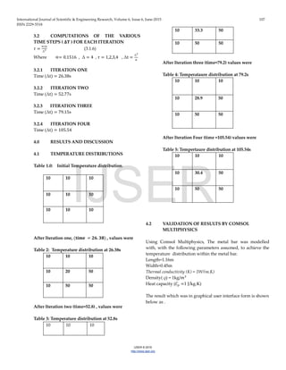
2.1 PROBLEM FORMULATION
An infinitely long bar of thermal diffusivity ᾳ has a cross sec-
tion of side 2a. It is initially at a uniform temperature 𝜃∘ and
then suddenly has its surface maintained at a temperature 𝜃1.
The subsequent temperatures 𝜃(𝑥, 𝑦, 𝑡) inside the bar are to be
solved and computed at various time-steps.
Dimensionless distances, time, and temperature are defined
by
𝑋 =
𝑥
𝑎
, 𝑌 =
𝑦
𝑎
, 𝜏 =
ᾳ𝑡
𝑎2
, 𝑎𝑎𝑎 𝑇 =
𝜃 − 𝜃∘
𝜃1 − 𝜃∘
Unsteady state conduction is governed by
𝜕2 𝑇
𝜕𝑋2
+
𝜕2 𝑇
𝜕𝑌2
=
𝜕𝑇
𝜕𝜏
2.2 BOUNDARY CONDITIONS
2.2.1 Initial Boundary Condition
𝜏 = 0: 𝑇 = 0 Throughout the region
2.2.2 Final Boundary Condition
𝜏 > 0: 𝑇 = 1 Along the sides 𝑋 = 1 𝑎𝑎𝑎 𝑌 = 1,
𝜕𝑇
𝜕𝑥
= 0 And
𝜕𝑇
𝜕𝑌
= 0
Along the sides 𝑋 = 0 𝑎𝑎𝑎 𝑌 = 0 respectively.
Figure 1.0: Initial temperature distributions of the sectioned
bar
Where 𝜃1 = 50°
𝐶
𝜃°=10°
𝐶
2.3 Elliptic equation
𝑇𝑥𝑥=
𝑇 𝑚−1,𝑛−2𝑇 𝑚,𝑛+𝑇 𝑚+1,𝑛
∆𝑋2
(2.3.1)
𝑇𝑦𝑦=
𝑇 𝑚,𝑛−1−2𝑇 𝑚,𝑛+𝑇 𝑚,𝑛+1
∆𝑌2
(2.3.2)
𝑇𝑥𝑥 + 𝑇𝑦𝑦 = 0 (2.3.3)
𝑇 𝑚−1,𝑛−2𝑇 𝑚,𝑛+𝑇 𝑚+1,𝑛
∆𝑋2
+
𝑇 𝑚,𝑛−1−2𝑇 𝑚,𝑛+𝑇 𝑚,𝑛+1
∆𝑌2
= 0 (2.3.4)
∆𝑋2
= ∆𝑌2
= ∆𝑍2
𝑇 𝑚,𝑛
𝑖+1
- 𝑇 𝑚,𝑛
𝑖
=
∝∆𝑡
∆2
[𝑇 𝑚+1,𝑛
𝑖
− 2𝑇 𝑚,𝑛
𝑖
+ 𝑇 𝑚−1,𝑛
𝑖
+𝑇 𝑚,𝑛+1
𝑖
− 2𝑇 𝑚,𝑛
𝑖
+
𝑇 𝑚,𝑛−1
𝑖
] (2.3.5)
But τ =
∝∆𝑡
∆2
3.0 COMPUTATION OF MESH FUNCTION ALONG
COLUMNS
𝑇 𝑚,𝑛
𝑖+1
− 𝑇 𝑚,𝑛
𝑖
= 𝜏�𝑇 𝑚+1,𝑛
𝑖
− 2𝑇 𝑚,𝑛
𝑖
+ 𝑇 𝑚−1,𝑛
𝑖 � + �𝑇 𝑚,𝑛+1
𝑖
− 2𝑇 𝑚,𝑛
𝑖
+ 𝑇 𝑚,𝑛−1
𝑖 � (3.0.1)
3.1 COMPUTATION OF MESH FUNCTION ALONG
ROWS
𝑇 𝑚,𝑛
𝑖+2
− 𝑇 𝑚,𝑛
𝑖+1
=τ[𝑇 𝑚+1,𝑛
𝑖+2
− 2𝑇 𝑚,𝑛
𝑖+2
+ 𝑇 𝑚−1,𝑛
𝑖+2
] + [𝑇 𝑚,𝑛+1
𝑖+1
− 2𝑇 𝑚,𝑛
𝑖+1
+ 𝑇 𝑚,𝑛−1
𝑖+1
]
(3.1.1)
For i = 1,2,3…..n-1 and j = 1,2,3…..n-1 , both equations yields a
tridiagonal system of equations.
At When 𝒊 = 𝟎 𝒂𝒂𝒂 𝒎 = 𝟏 and 𝒏 = 𝟏
−𝜏𝑇1,2
(1)
+ [1 + 2𝜏]𝑇1,1
(1)
− 𝜏𝑇1,0
(1)
= 𝜏𝑇0,1
(1)
+ [1 − 2𝜏]𝑇1,1
(0)
+ 𝜏𝑇2,1
(0)
(3.1.2)
3.1.1 ITERATION ONE (𝝉 = 𝟏)
−𝜏50 + [1 + 2𝜏]𝑇1,1
(1)
− 1 0 = 0 + [1 − 2𝜏]0 + 0
𝑇1,1
(1)
= 20
3.1.2 ITERATION TWO
Equation (a) was used in computing 𝑇1,1
(1)
.
It’s direction was alternated and used in computing the func-
tion value for 𝑇1,1
(2)
on the row, using equation (b)
−𝑇 𝑚−1,𝑛
𝑖+2
+ 3𝑇 𝑚,𝑛
𝑖+2
− 𝑇 𝑚+1,𝑛
𝑖+2
= 𝑇 𝑚,𝑛+1
𝑖+1
− 𝑇 𝑚,𝑛
𝑖+1
+ 𝑇 𝑚,𝑛−1
𝑖+1
(3.1.3)
When i = 0 , n = 1 and m = 1
−𝑇0,1
(2)
+ 3𝑇1,1
(2)
− 𝑇2,1
(2)
= 𝑇1,2
(1)
− 𝑇1,1
(1)
+ 𝑇1,0
(1)
𝑇1,1
(2)
= 33.3
3.1.3 ITERATION THREE
equation (a) and (c) yields
−𝜏𝜏 𝑚,𝑛+1
𝑖+1
+ [1 + 2𝜏]𝑇 𝑚,𝑛
𝑖+1
− 𝜏𝜏 𝑚,𝑛−1
𝑘+1
= 𝜏𝜏 𝑚−1,𝑛
𝑖
+ [1 − 2𝜏]𝑇 𝑚,𝑛
𝑖
+ 𝜏𝜏 𝑚+1,𝑛
𝑖
(3.1.4)
When i=2, m=1 and j=1
[1 + 2𝜏]𝑇1,1
(3)
= 𝜏10 + 𝜏10 + 𝜏50 + 𝜏50 + [1 − 2𝜏]33.3
(𝝉 = 𝟏)
3𝑇1,1
(3)
= 10 + 10 + 50 + 50 + [1 − 2]33.3
𝑇1,1
(3)
= 28.9
3.1.4 ITERATION FOUR
𝐞𝐞𝐞𝐞𝐞𝐞𝐞𝐞 (𝐛) 𝐚𝐚𝐚 (𝐟) 𝐚𝐚𝐚 𝐝𝐝𝐝𝐝𝐝𝐝𝐝 𝐚𝐚
−𝑇 𝑚−1,𝑛
𝑖+2
+ 3𝑇 𝑚,𝑛
𝑖+2
− 𝑇 𝑚+1,𝑛
𝑖+2
= 𝑇 𝑚,𝑛+1
𝑖+1
− 𝑇 𝑚,𝑛
𝑖+1
+ 𝑇 𝑚,𝑛−1
𝑖+1
(3.1.5)
𝒘𝒘𝒘𝒘 𝒊 = 𝟐 , 𝒏 = 𝟏 𝒂𝒂𝒂 𝒎 = 𝟏
−𝑇0,1
(4)
+ 3𝑇1,1
(4)
− 𝑇2,1
(4)
= 𝑇1,2
(3)
− 𝑇1,1
(3)
+ 𝑇1,0
(3)
𝑇1,1
(4)
= 30.4
IJSER

3. International Journal of Scientific & Engineering Research, Volume 6, Issue 6, June-2015 107
ISSN 2229-5518
IJSER © 2015
http://www.ijser.org
3.2 COMPUTATIONS OF THE VARIOUS
TIME STEPS ( 𝚫𝚫 ) FOR EACH ITERATION
𝜏 =
∝Δt
Δ2 (3.1.6)
Where ∝= 0.1516 , Δ = 4 , 𝜏 = 1,2,3,4 , Δt =
Δ2
∝
3.2.1 ITERATION ONE
Time (Δt) = 26.38s
3.2.2 ITERATION TWO
Time (Δt) = 52.77s
3.2.3 ITERATION THREE
Time (Δt) = 79.15s
3.2.4 ITERATION FOUR
Time (Δt) = 105.54
4.0 RESULTS AND DISCUSSION
4.1 TEMPERATURE DISTRIBUTIONS
Table 1.0: Initial Temperature distribution.
10 10 10
10 10 10
10 10 10
After Iteration one, (𝐭𝐭𝐭𝐭 = 𝟐𝟐. 𝟑𝟑) , values were
Table 2: Temperature distribution at 26.38s
10 10 10
10 20 50
10 50 50
After Iteration two (time=52.8) , values were
Table 3: Temperature distribution at 52.8s
10 10 10
10 33.3 50
10 50 50
After Iteration three (time=79.2) values were
Table 4: Temperataure distribution at 79.2s
10 10 10
10 28.9 50
10 50 50
After Iteration Four (time =105.54) values were
Table 5: Tempertaure distribution at 105.54s
10 10 10
10 30.4 50
10 50 50
4.2 VALIDATION OF RESULTS BY COMSOL
MULTIPHYSICS
Using Comsol Multiphysics, The metal bar was modelled
with, with the following parameters assumed, to achieve the
temperature distribution within the metal bar.
Length=1.16m
Width=0.45m
Thermal conductivity (K) = 1W/(m.K)
Density( ρ) = 1kg/𝑚3
Heat capacity (𝐶𝜌 =1 J/kg.K)
The result which was in graphical user interface form is shown
below as .
IJSER

4. International Journal of Scientific & Engineering Research, Volume 6, Issue 6, June-2015 108
ISSN 2229-5518
IJSER © 2015
http://www.ijser.org
Figure 2: Temperature distribution within the metal bar
Figure 3: Isothermal contour showing temperature distri-
bution within the metal bar
Figure 4: A comparison of ADI results with COMSOL
results
CONCLUSIONS
The two Dimensional Heat problem was modelled using
COMSOL MULTIPHYSICS which gave a graphical distribu-
tion of temperature within the metal and a graph showing the
convergence of the finite difference iterative scheme.
The ADI iterative scheme was highly effective in determin-
ing the nodal temperatures within the sectioned metal bar.
On comparing the Modelled results from COMSOL MUL-
TIPHYSICS and the results from ADI iterative scheme, there
was an high level of agreement between both results , notably
if one observe closely the results for node 𝑇1,1
1
=20, 𝑇1,1
2
=33.3 ,
𝑇1,1
3
=28.9 , 𝑇1,1
4
=30.4 with the temperature distribution of the
Mid-section of the Metal Bar with COMSOL MULTIPHYSICS,
a large level of conformity exists.
For problems with a simple geometry, the ADI finite differ-
ence method
is cost-effective with stability and accuracy similar to the
finite-element methods.
ACKNOWLEDGMENT
The authors are grateful to Dr. Falana for guidance and as-
sistance on this work.
REFERENCES
1. Comparison of Numerical Modeling Techniques for Complex,.
Thomas, B. G, SAMARASEKERA, I. V and BRIMACOMBE,
J. K. 1984, METALLURGICAL TRANSACTIONS B, Vol. 15B,
pp. 307-318.
2. AFSHEEN, ARIF. ALTERNATING DIRECTION IMPLIC-
IT METHOD FOR TWO-DIMENSIONAL HEAT TRANSFER
PROBLEM. National College of Business Administration&
Economics. LAHORE : s.n., 2OO9. pp. 1-90.
3. A FORMULATION OF PEACHMAN AND RACHFORD
ADI METHOD FOR THE THREE-DIMENSIONAL HEAT DIF-
FUSION EQUATION. Ismail, I. A, Zahran, E. H and Shehata,
M. 2004, Mathematical and Computational Applications, Vol.
9, pp. 183-189.
4. An alternating direction implicit method for a second-order.
Adérito, Araújo, Cidália, Neves and Ercília, Sousa. s.l. :
ELSEVIER, 2014, Applied Mathematics and Computation, Vol.
239, pp. 17-28.
5. ALTERNATING DIRECTION IMPLICIT METHODS FOR
TWO-DIMENSIONAL DIFFUSION WITH A NON-LOCAL
BOUNDARY CONDITION. DEHGHAN, M. s.l. : Overseas
Publishers Association, 1998, International Journal of Comput-
er Mathematics, Vol. 72, pp. 349-366.
6. AN ALTERNATING DIRECTION IMPLICIT METHOD
APPLIED TO THE CALCULATION OF A MAGNETIC FIELD
FROM A MEASURED BOUNDARY. Groth, T, Olsen, B and
PETTERSSON, G. [ed.] 56. s.l. : NORTH-HOLLAND PUB-
LISHING CO., 1967, NUCLEAR INSTRUMENTS AND
METHODS, pp. 61-68.
7. Cengel, Yunus. A. Heat and Mass Transfer: A practical ap-
proach. 2006.
IJSER