ANN

1. 1
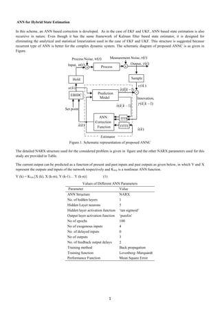
ANN for Hybrid State Estimation
In this scheme, an ANN based correction is developed. As in the case of EKF and UKF, ANN based state estimation is also
recursive in nature. Even though it has the same framework of Kalman filter based state estimator, it is designed for
eliminating the analytical and statistical linearization used in the case of EKF and UKF. This structure is suggested because
recurrent type of ANN is better for the complex dynamic system. The schematic diagram of proposed ANNC is as given in
Figure.
Figure.1. Schematic representation of proposed ANNC
The detailed NARX structure used for the considered problem is given in figure and the other NARX parameters used for this
study are provided in Table.
The current output can be predicted as a function of present and past inputs and past outputs as given below, in which Y and X
represent the outputs and inputs of the network respectively and KNN is a nonlinear ANN function.
Y (k) = KNN{X (k), X (k-m), Y (k-1)… Y (k-n)} (1)
Values of Different ANN Parameters
Parameter Value
ANN Structure NARX
No. of hidden layers 1
Hidden Layer neurons 5
Hidden layer activation function ‘tan sigmoid’
Output layer activation function ‘purelin’
No of epochs 100
No of exogenous inputs 4
No. of delayed inputs 0
No of outputs 3
No. of feedback output delays 2
Training method Back propagation
Training function Levenberg–Marquardt
Performance Function Mean Square Error
Process Noise,
Set point
Input,
Measurement Noise,
Output,
Prediction
Model
ANN
Correction
Function
ITD
OTD
EBIDC
Innovation,
xk/k-1
Process
SampleHold
Estimator

2. 2
A sequence of current and past input vectors (X (k), X (k-1), X (k-m)) are obtained by passing X (k) through an input time
delay unit, ITD (0: m). Similarly output time delay unit, OTD (1: n) provides a sequence of past output vectors (Y (k-1), Y (k-
n)). For the considered problem, the input and the output are T
1 2 3
ˆ ˆ ˆX( ) [ ( 1), ( 1), ( 1), ( 1)]    k h k k h k k h k k k k
T
1 2 3
ˆ ˆ ˆY( ) [ ( ), ( ), ( )]k h k h k h k respectively.
Similar to Kalman filter based state estimators and its nonlinear extensions; proper value for the initial state vector is assumed
for the prediction model. The input and output measurements are made from the process and the input measurement are
presented to the prediction model along with the assumed initial state vector in order to compute the time updated values for
states.
ˆ ˆ( 1) F( ( 1), ( ))  x k k x k u k (2)
With, ˆ ˆ( 1) (0) [ (0)]  x k x E x , the assumed initial value of state vector.
This a priori state estimates, ˆ( 1)x k k can be given to the output model so that a priori estimates of the output, ˆ( 1)y k k can
be obtained as
ˆ ˆ( 1) H ( 1)    y k k x k k (3)
The innovation between plant output, ( )y k and a priori output estimates, ˆ( 1)y k k is calculated as
ˆ( 1) ( ) ( 1)   k k y k y k k (4)
In the correction step of the algorithm, the a priori state estimates will be corrected using this innovation with the help of the
ANN to obtain a posteriori estimates of states
.
Figure.2. NARX structure for the considered example
 NNˆ ˆ ˆ( ) K ITD( ( 1), ( 1)),OTD( ( ))  x k x k k k k x k (5)

3. 3
These estimated states are fed back to the controller for calculating the new input signal to the plant. For the next iteration, a
posteriori estimate of state can be given to the prediction model (instead of assumed initial states as in the first iteration) along
with the new input measurement from the plant. This can be continued for the entire process run
Experimental Results and Performance Analysis
Real-time experimental validations were carried out on the experimental setup. In addition to the experimental setup, other
tools used, which were for the real time implementation are the software Lab VIEW and the NI DAQ pad (USB6251). In the
real system, the performance of the controller in regulatory operation and servo operation based on ISE and average
computation time per iteration is shown in figure. Response of the system in initial condition mismatch is shown. The response
of the system in +10% and -10% plant model parameter mismatch is given below. Results of hand valve faults which can occur
in real time application are given in Tables. The real time experimental results support the simulation results on performance.
Regulatory Control Problem: Controller Performance Comparison
Controller ISE(h1) ISE(h2)
Avg. Computation
time per iteration (S)
Proposed 0.0200 0.0193 0.1038
Servo Control Problem: Controller Performance Comparison
Controller ISE(h1) ISE(h2)
Avg. Computation
time per iteration (S)
Proposed 0.0172 0.0144 0.1152
Initial Condition Mismatch: Controller Performance Comparison
Controller ISE(h1) ISE(h2)
Avg. Computation
time per iteration (S)
Proposed 0.0214 0.0592 0.1017
Plant Model Parameter Mismatch (+10%): Controller Performance Comparison
Controller ISE(h1) ISE(h2)
Avg. Computation
time per iteration (S)
Proposed 0.0045 0.0069 0.2112
Plant Model Parameter Mismatch (-10%): Controller Performance Comparison
Controller ISE(h1) ISE(h2)
Avg. Computation
time per iteration (S)
Proposed 0.0122 0.0131 0.1037
Hand Valve Faults -Leakage: Controller Performance Comparison
Controller ISE(h1) ISE(h2)
Avg. Computation
time per iteration (S)
Proposed 0.0600 0.0077 0.0768

4. 4
Hand Valve Faults -Clogging: Controller Performance Comparison
Controller ISE(h1) ISE(h2)
Avg. Computation
time per iteration (S)
Proposed 0.0082 0.0078 0.0943
Regulatory response of hybrid three tank system with ANNC (a) Level in Tank 1, (b) Level in tank 2
Servo response of hybrid three tank system with ANNC (a) Level in Tank 1, (b) Level in tank 2
50 100 150 200 250 300 350 400
0.24
0.27
0.3
0.33
Level(h
1
)
(a)
CV1
(Proposed) SETPOINT1
100 200 300 400
0.24
0.27
0.3
0.33
Level(h
2
)
(b)
Sampling Instants
CV2
(Proposed) SETPOINT2
50 100 150 200
0.23
0.26
0.29
0.32
Level(h
1
)
(a)
50 100 150 200
0.23
0.26
0.29
0.32
Level(h
2
)
(b)
Sampling Instants
CV2
(Proposed) SETPOINT2
CV1
(Proposed) SETPOINT1
50 100 150 200 250 300 350 400
0.26
0.3
0.34
0.38
Level(h
1
)
(a)
CV1
(Proposed) SETPOINT1
50 100 150 200 250 300 350 400
0.26
0.3
0.34
0.38
Level(h
2
)
(b)
Sampling Instants
CV2
(Proposed) SETPOINT2

5. 5
Closed response of hybrid three tank system with ANNC (Initial Condition Mismatch ) (a) Level in Tank 1, (b) Level in Tank 2
Closed response of hybrid three tank system with ANNC (Plant-Model mismatch +10% ) (a) Level in Tank 1, (b) Level in Tank 2
Closed response of hybrid three tank system with ANNC (Plant-Model mismatch -10% ) (a) Level in Tank 1, (b) Level in Tank 2
Closed response of hybrid three tank system with ANNC (Handvalve fault-Leakage ) (a) Level in Tank 1, (b) Level in Tank 2
50 100 150 200 250
0.28
.3
0.32
Level(h
1
)
(a)
CV1
(Proposed) SETPOINT1
50 100 150 200 250
0.28
0.3
0.32
Level(h
2
)
(b)
Sampling Instants
CV2
(Proposed) SETPOINT2
50 100 150 200 250
0.26
0.28
0.3
0.32
Level(h
1
)
(a)
CV1
(Proposed) SETPOINT1
50 100 150 200 250
0.26
0.28
0.3
0.32
Level(h
2
)
(b)
Sampling Instants
CV2
(Proposed) SETPOINT2
100 200 300 400 500
0.26
0.28
Level(h
1
)
(a)
100 200 300 400 500
0.26
0.28
Level(h
2
)
(b)
Sampling Instants
CV2
(Proposed) SETPOINT2
CV1
(Proposed) SETPOINT1

6. 6
Closed response of hybrid three tank system with ANNC (Handvalve fault-Clogging ) (a) Level in Tank 1, (b) Level in Tank 2
50 100 150 200 250
0.25
0.3
0.35
Level(h
1
)
(a)
100 200 300 400 500
0.25
0.3
0.35
Level(h
2
)
(b)
Sampling Instants
CV2
(Proposed) SETPOINT2
CV1
(Proposed) SETPOINT1