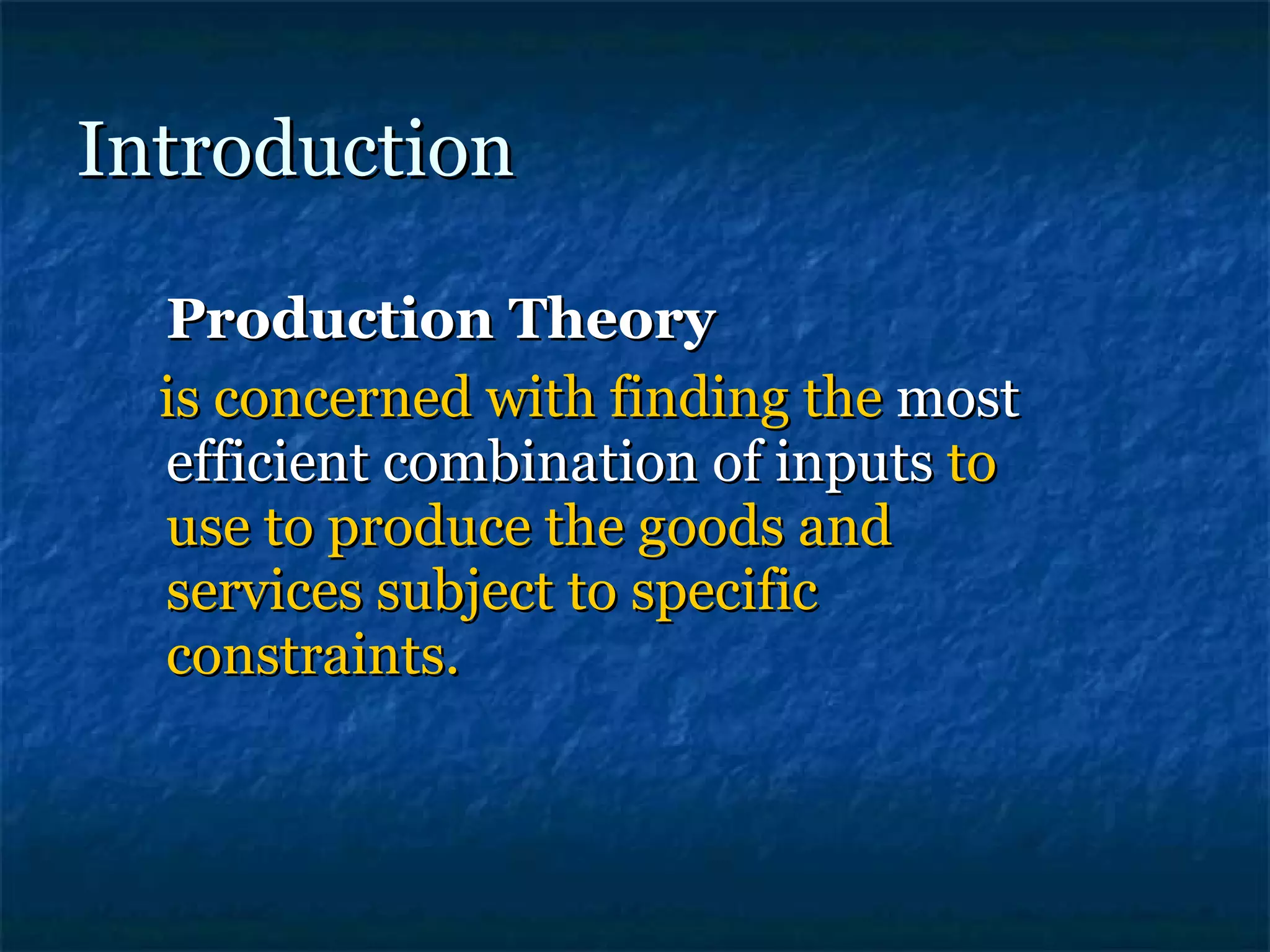
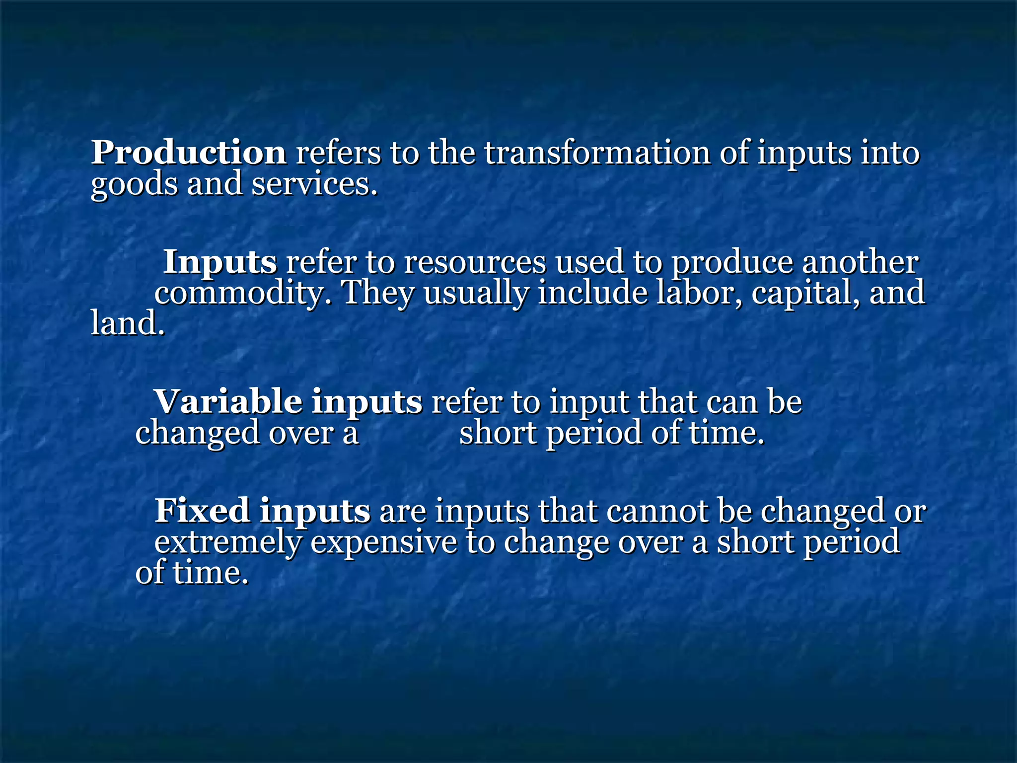
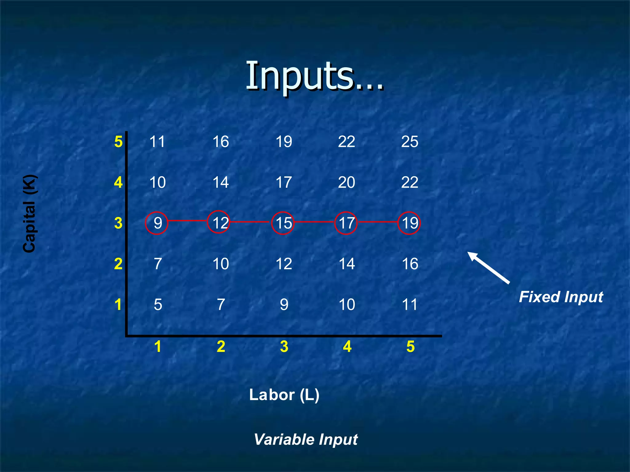
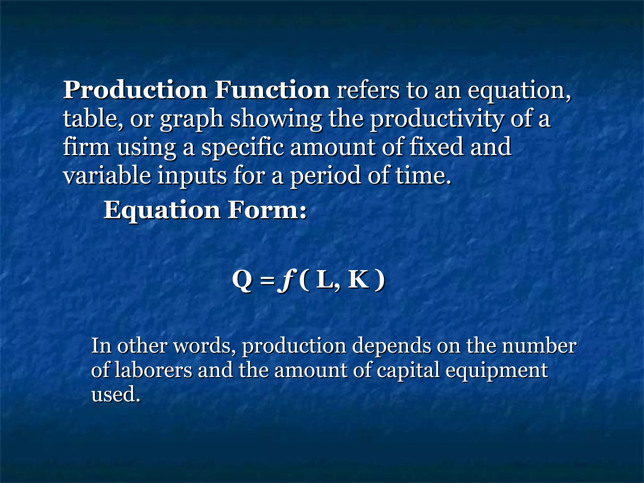
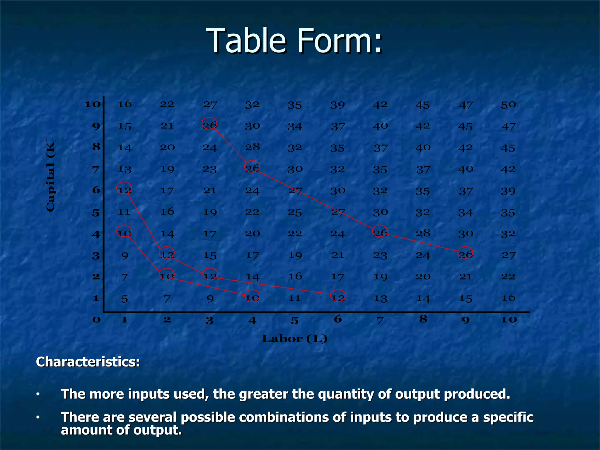
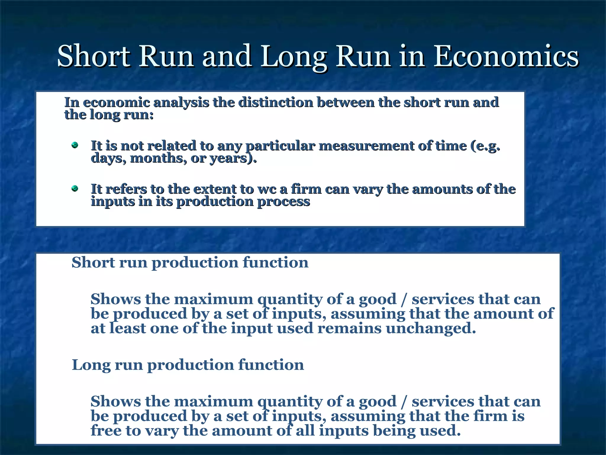
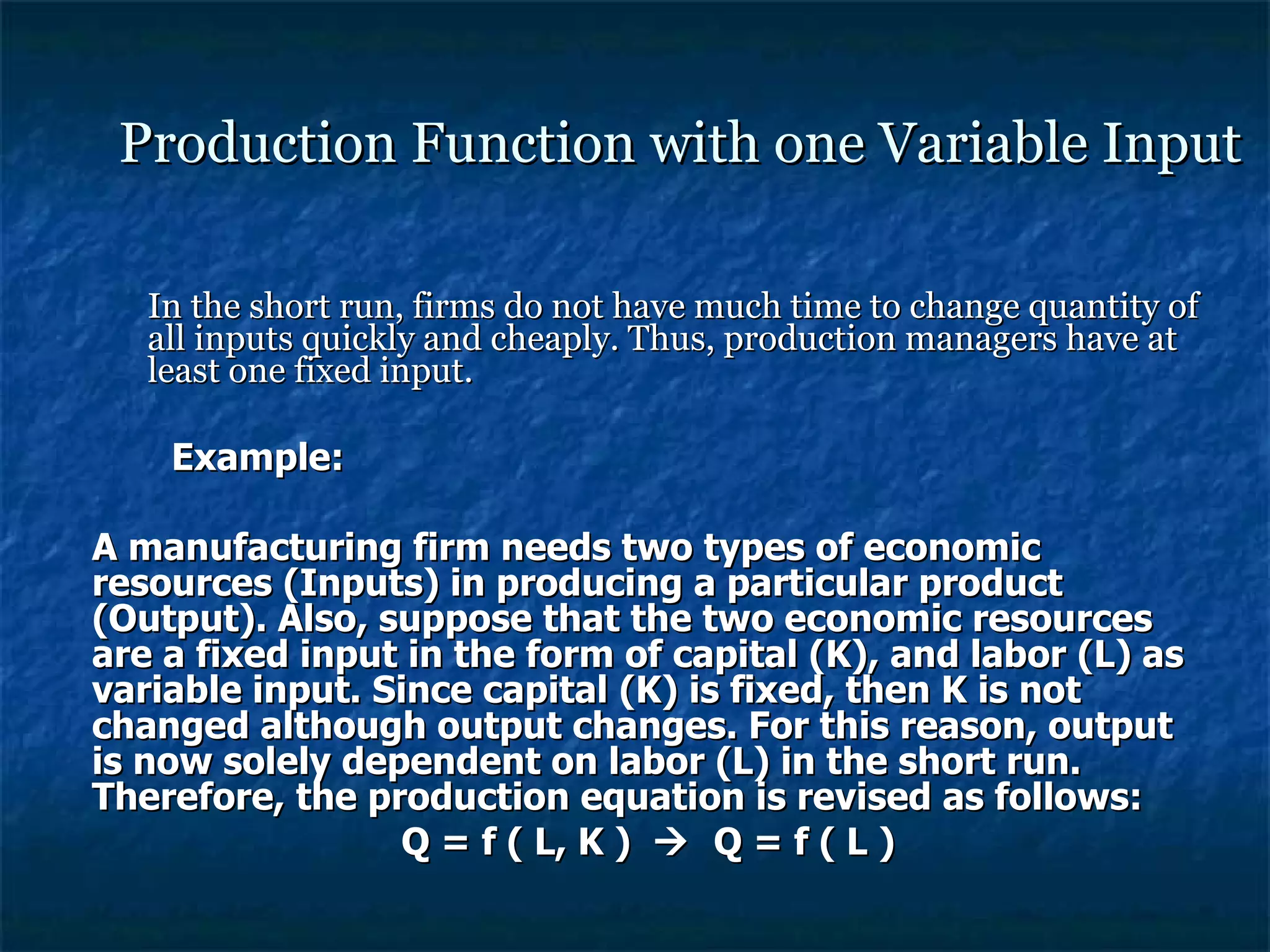
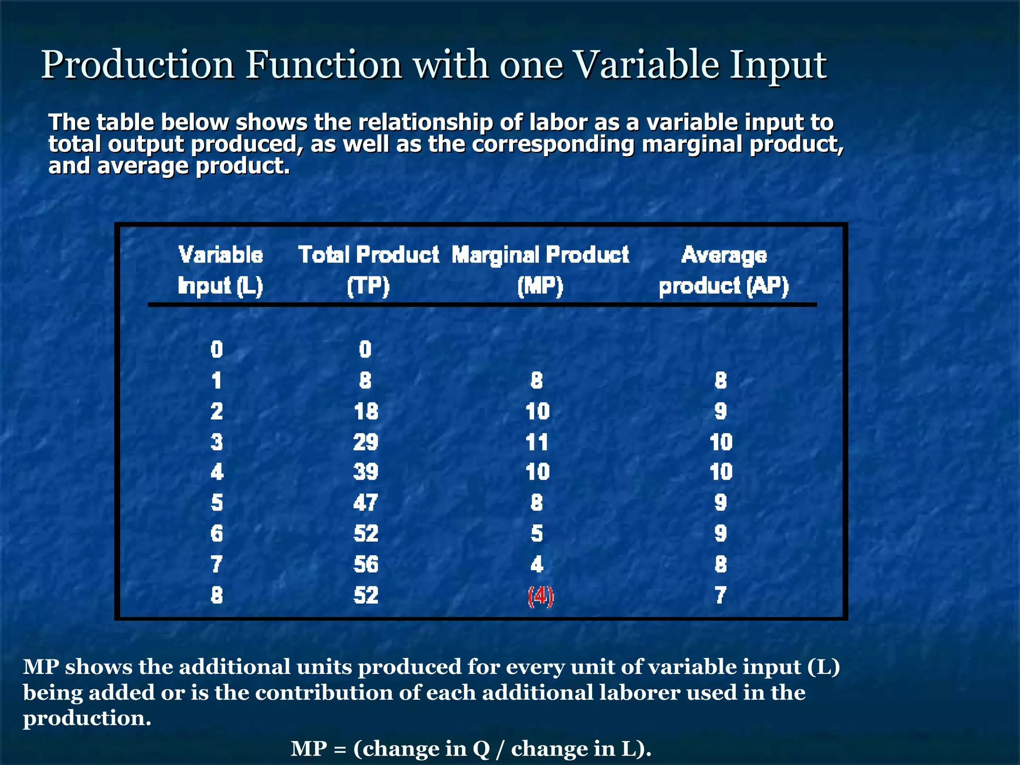
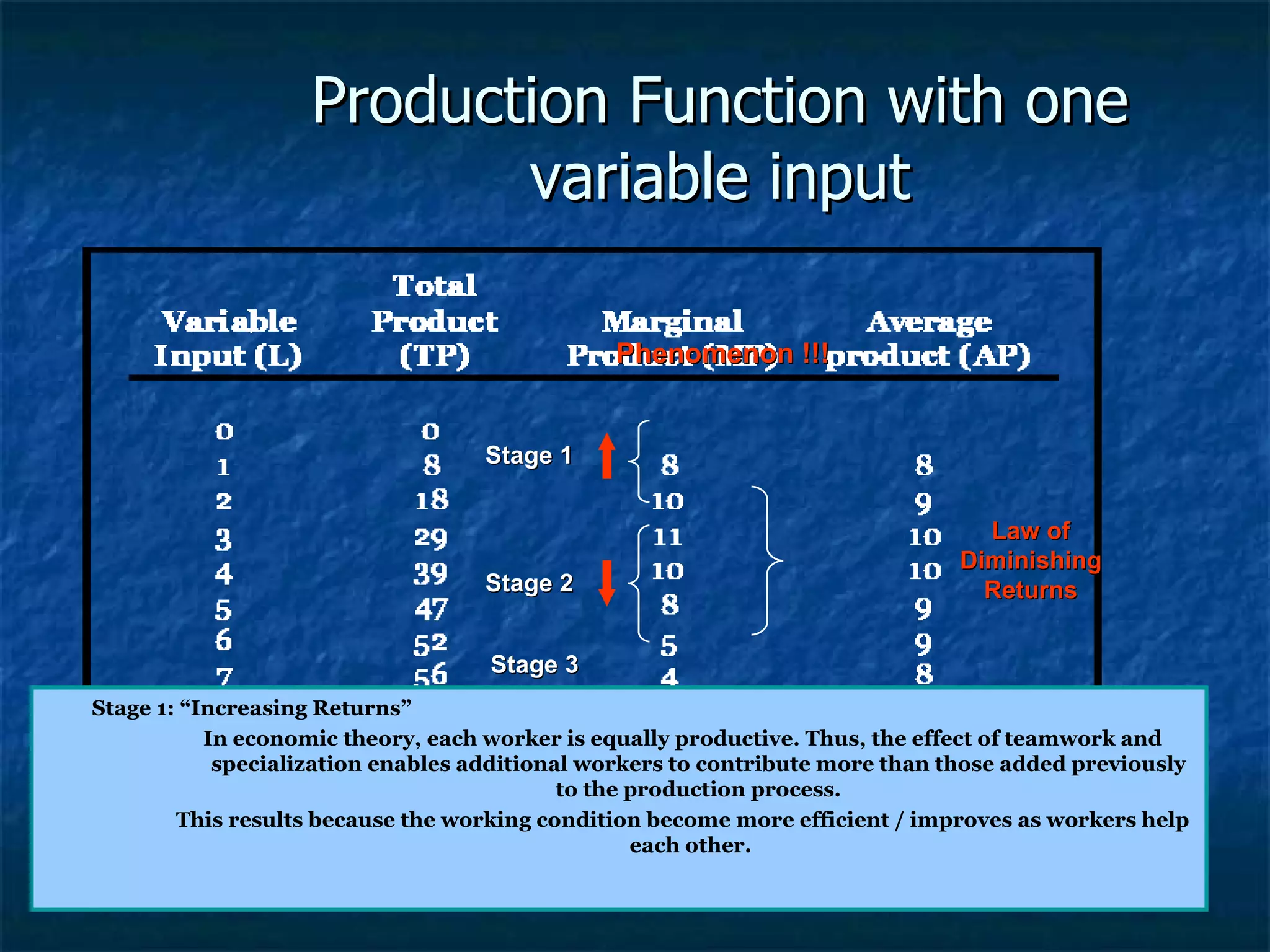
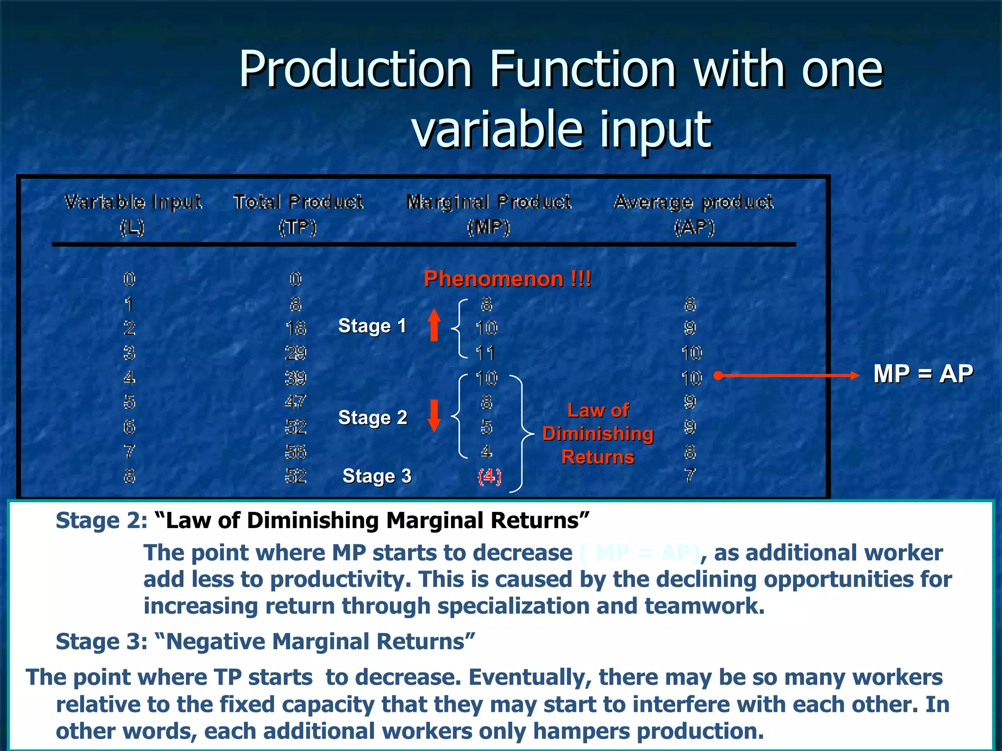
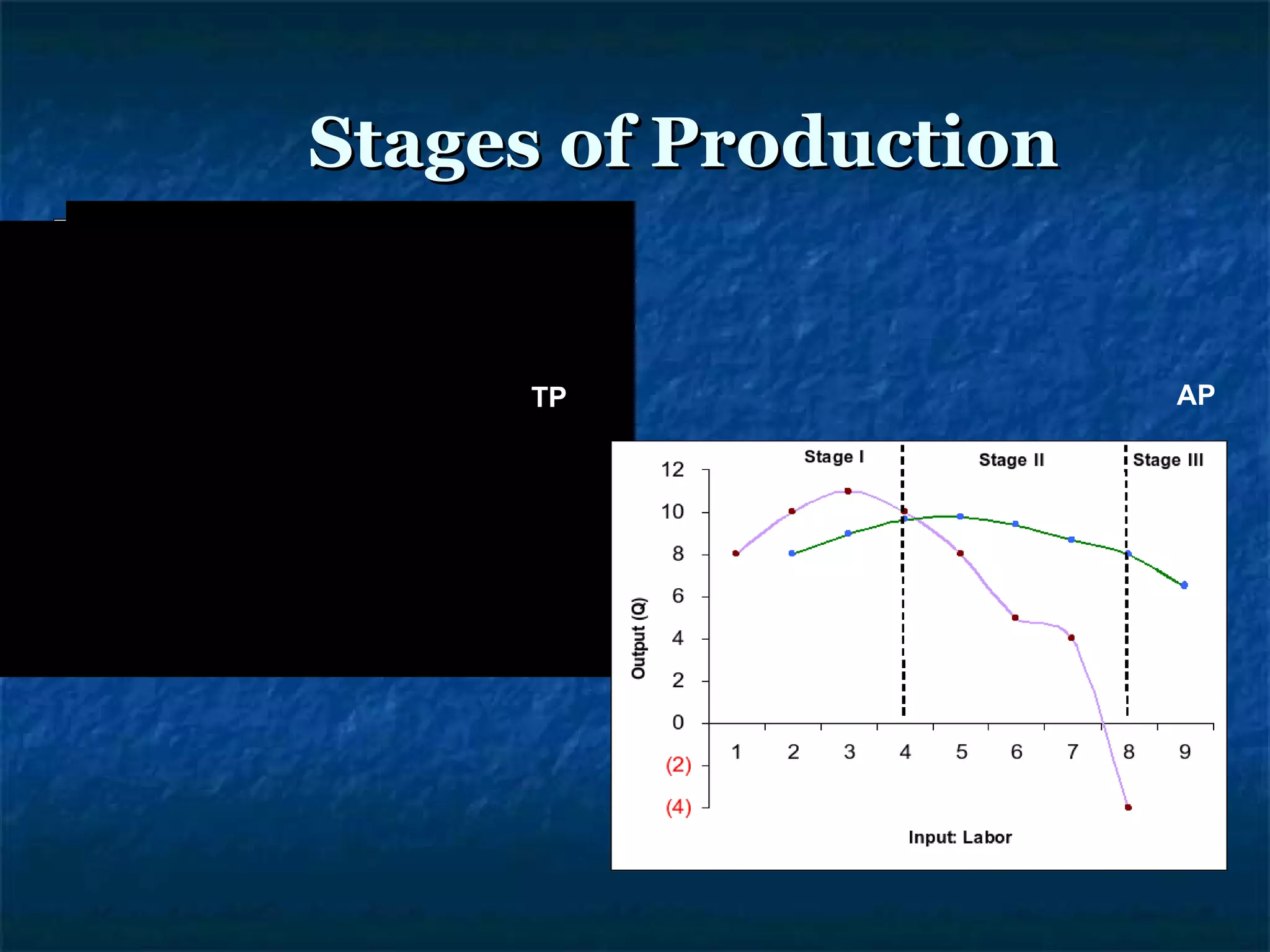
Production theory is concerned with finding the most efficient combination of inputs to produce goods and services given constraints. Inputs include labor, capital, and land, which are used to produce outputs in the form of intermediate and final goods. The production function shows the relationship between inputs and maximum possible output in the short and long run. In the short run, at least one input is fixed, so output depends on the variable input. The law of diminishing returns states that adding more of the variable input initially increases, then decreases, marginal product.

1. PRODUCTION THEORY [email_address]

2. Introduction Production Theory is concerned with finding the most efficient combination of inputs to use to produce the goods and services subject to specific constraints.

3. Production refers to the transformation of inputs into goods and services. Inputs refer to resources used to produce another commodity. They usually include labor, capital, and land. Variable inputs refer to input that can be changed over a short period of time. Fixed inputs are inputs that cannot be changed or extremely expensive to change over a short period of time.

4. Inputs… Fixed Input Variable Input

5. Outputs are the goods or services produced which may either be in the form of an intermediary goods and final goods. Intermediate goods refer to products used as input goods; also called as capital / producers / investment goods that are used in production of other goods. Final goods are products used in consumption; Consumer goods.

6. Production Function refers to an equation, table, or graph showing the productivity of a firm using a specific amount of fixed and variable inputs for a period of time. Equation Form: Q = f ( L, K ) In other words, production depends on the number of laborers and the amount of capital equipment used.

7. Table Form: Characteristics: The more inputs used, the greater the quantity of output produced. There are several possible combinations of inputs to produce a specific amount of output.

8. In economic analysis the distinction between the short run and the long run: It is not related to any particular measurement of time (e.g. days, months, or years). It refers to the extent to wc a firm can vary the amounts of the inputs in its production process Short Run and Long Run in Economics Short run production function Shows the maximum quantity of a good / services that can be produced by a set of inputs, assuming that the amount of at least one of the input used remains unchanged. Long run production function Shows the maximum quantity of a good / services that can be produced by a set of inputs, assuming that the firm is free to vary the amount of all inputs being used.

9. Production Function with one Variable Input In the short run, firms do not have much time to change quantity of all inputs quickly and cheaply. Thus, production managers have at least one fixed input. Example: A manufacturing firm needs two types of economic resources (Inputs) in producing a particular product (Output). Also, suppose that the two economic resources are a fixed input in the form of capital (K), and labor (L) as variable input. Since capital (K) is fixed, then K is not changed although output changes. For this reason, output is now solely dependent on labor (L) in the short run. Therefore, the production equation is revised as follows: Q = f ( L, K )  Q = f ( L )

10. Production Function with one Variable Input The table below shows the relationship of labor as a variable input to total output produced, as well as the corresponding marginal product, and average product. MP shows the additional units produced for every unit of variable input (L) being added or is the contribution of each additional laborer used in the production. MP = (change in Q / change in L). AP represents the average unit produced by each laborer given the different levels of variable input. In other words, it represents the productivity of each worker on average. AP = ( Q / L).

11. Production Function with one variable input Stage 1: “Increasing Returns” In economic theory, each worker is equally productive. Thus, the effect of teamwork and specialization enables additional workers to contribute more than those added previously to the production process. This results because the working condition become more efficient / improves as workers help each other. Phenomenon !!! Law of Diminishing Returns Stage 1 Stage 2 Stage 3

12. Production Function with one variable input Stage 2: “Law of Diminishing Marginal Returns” The point where MP starts to decrease ( MP = AP) , as additional worker add less to productivity. This is caused by the declining opportunities for increasing return through specialization and teamwork. Stage 3: “Negative Marginal Returns” The point where TP starts to decrease. Eventually, there may be so many workers relative to the fixed capacity that they may start to interfere with each other. In other words, each additional workers only hampers production. Phenomenon !!! Law of Diminishing Returns MP = AP Stage 1 Stage 2 Stage 3

13. Stages of Production TP AP MP