Production function- Law of variable proportions - Applications of Law of variable proportions - Law of returns to scale - Constant returns to scale - Increasing to returns scale - Decreasing to returns scale - Economies of scale - Internal economies of scale - External economies of scale - Cost classification

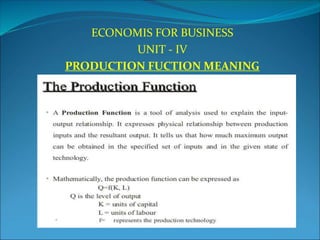
1. ECONOMIS FOR BUSINESS
UNIT - IV
PRODUCTION FUCTION MEANING

2. PRODUCTION FUCTION

3. Short run and long run
Short run refers to a time period in which a firm
does not have sufficient time to increase the scale
of output. It can increase only the level of output
by increasing the quantity of a variable factor and
making intensive use of the existing fixed factors.
On the other hand long run refers to the time
period in which the firms can increase the scale of
output by increasing the quantity of all the factor
inputs simultaneously and in the same proportion.
The distinction between fixed and variable factors
is relevant only in the short run but this distinction
disappears in the long run.

4. Fixed factors and variable factors
Fixed factors are those factors of production whose
quantity can not be hanged with change in the level of
output. For example, the quantity of land, machinery
etc. can not be hanged during short run.
On the other hand, variable factors are those factors of
production whose quantity can easily be hanged with
change in the level of output. For example, we can
easily change the quantity of labour to increase or
decrease the production.

5. Level of production and scale of production
When any firm increases production by increasing
the quantity of one factor input where as the
quantity of other factor inputs keeping constant; it
increases the level of production. But on the other
hand, when the firms increases production by
increasing the quantity of all the factors of
production simultaneously and in the same
proportion, it increases the scale of production.

6. we have to understand the three measures of production
and their relationships because without understanding
these measure of production, the concepts of laws of
production can not be clearly understood.
There are mainly the following three measures of
production:
 Total product or total physical product denoted by TPP.
 Average Product (AP) or Average physical produt
denoted by APP.
 Marginal Product (MP) or marginal physical product
denoted by MPP.

7. Total Physical Product (TPP)
TPP is the total amount of a commodity that is
produced with a given level of factor inputs and
technology during a given period of time. For
example, 2 units of labour combined with 2 units of
capital can produce 26 fans per day. Here 26 fans is
the total physical produt which is produced with the
given level of inputs (labour and capital)

8. Average Physical Product (APP)
APP is the output produced per unit of input
employed. It can be obtained by dividing TPP by the
number of units of variable input. So APP = TPP/L
where L is the units of labour. For example, if 10
workers make 30 chairs per day, the APP of a worker
per day will be 30 ÷ 10 = 3 chairs. If the productivity
of a factor increases, it implies that the output per unit
of input has increased.

9. Marginal Physical Product (MPP)
MPP of an input is the additional output that can
be produced by employing one more unit of that
input while keeping other inputs constant. For
example, if ten tailors can make 50 shirts per day
and 11 tailors can make 54 shirts per day, the
marginal product of 11 workers will be 54 - 50 = 4
shirts per day.

11. LAW OF VARIABLE PROPORTIONS
The law of variable proportions is a short
period production law. It is also called returns
to a factor. Let us first understand the meaning
of variable proportions. In a production
process when only one factor is varied and all
other factors remain constant, as more and
more units of variable factor are employed, the
proportion between fixed and variable factors
goes on changing. So it is termed as the law of
variable proportions.

12. This law states that if you go on using more and
more units of variable factor (labour) with fixed
factor (capital), the total output initially increases at
an increasing rate but beyond a certain point, it
increases at a diminishing rate and finally it falls. This
law was initially called the law of dimiting returns
Marshall who applied the law only in agriculture sector
but modern economist called it the law of variable
proprotion and proposed its applicability to all the
sectors of the economy.

13. Assumption of the law
The law operates under the following assumptions:
The firm operates in the short run.
There is no change in technology of production.
The production process allows the different factor
ratios to produce different levels out output.
All the units of variable factor are equally
efficient.
Full substitutability of factors of production is not
possible.

14. Applicability of the law of Variable Proportion
Law of variable
proportions applies to all fields of production,
like agriculture, industry, etc. This law applies
to any field of production where some factors
are fixed and other are variable. That is the
reason, why it is called law of universal
application.
Application to Agriculture
Application to Industry

15. LAW OF RETURN TO SCALE AND IT’S TYPES (WITH
DIAGRAM)
The law of returns to scale explains the
proportional change in output with respect to
proportional change in inputs. In other words, the law of
returns to scale states when there are a proportionate
change in the amounts of inputs, the behavior of output
also changes.
The degree of change in output varies with change
in the amount of inputs. For example, an output may
change by a large proportion, same proportion, or small
proportion with respect to change in input.

16. On the basis of these possibilities, law of
returns can be classified into three
categories:
i. Increasing returns to scale
ii. Constant returns to scale
iii. Diminishing returns to scale

17. INCREASING RETURNS TO SCALE
If the proportional change in the output of an
organization is greater than the proportional change in
inputs, the production is said to reflect increasing
returns to scale. For example, to produce a particular
product, if the quantity of inputs is doubled and the
increase in output is more than double, it is said to be
an increasing returns to scale. When there is an
increase in the scale of production, the average cost
per unit produced is lower. This is because at this stage
an organization enjoys high economies of scale.

18. shows the increasing returns to
scale:

19. CONSTANT RETURNS TO SCALE
The production is said to generate constant returns to
scale when the proportionate change in input is equal
to the proportionate change in output. For example,
when inputs are doubled, so output should also be
doubled, then it is a case of constant returns to scale.

20. DIMINISHING RETURNS TO SCALE
Diminishing returns to scale refers to a situation when the
proportionate change in output is less than the
proportionate change in input. For example, when capital
and labor is doubled but the output generated is less than
doubled, the returns to scale would be termed as
diminishing returns to scale.
shows the diminishing returns to scale:

21. ECONOMIES OF THE SCALE
Economies of the Scale of Production
According to Stinger, Economies of scales is synonyms of
returns to scale. When scale of production is increased, up
to a point, one gets economies of scale. Therefore,
diseconomies of scale follow. Increasing returns to scale
is the result of these economies. Marshall has divided
economies of scale into two parts :-
A.Internal Economies
B.External Economies

22. INTERNAL ECONOMIES
Internal economies of scale are those economies
which are internal to the firm. These arise within the
firm as a result of increasing the scale of output of the
firm. A firm secures these economies from the growth
of the firm independently. The main internal
economies are grouped under the following heads:
Technical Economies
Managerial Economies
Marketing Economies
Financial Economies
Risk Bearing Economies
Economies of Scale:

23. EXTERNAL ECONOMIES
External economies of scale are those
economies which are not specially availed of by
.any firm. Rather these accrue to all the firms in
an industry as the industry expands. • The main
external economies are as under:
Economies of localization.
Economies of vertical disintegration.
Economies of information.
Economies of by products.

24. EXTERNAL ECONOMIES
External economies of scale are those
economies which are not specially availed of by
.any firm. Rather these accrue to all the firms in
an industry as the industry expands. • The main
external economies are as under:
Economies of localization.
Economies of vertical disintegration.
Economies of information.
Economies of by products.

25. COST CLASSIFICATION
Cost classification is the logical process of categorising the
different costs involved in a business process according to
their type, nature, frequency and other features to fulfil
accounting objectives and facilitate economic analysis. Cost
refers to the value sacrificed with the aim of gaining
something in return. Every business process involves some
cost. It is the basis of profit determination for an
organisation. Knowing about the different expenses facilitate
the procedure of cost accounting in an organization. A
particular cost can be allocated under multiple categories.
For instance; salary paid to an employee is a labour cost as
well as a fixed cost. Moreover, the different elements of cost
classification are linked to each other in one or the other
way.

26. Cost Classification