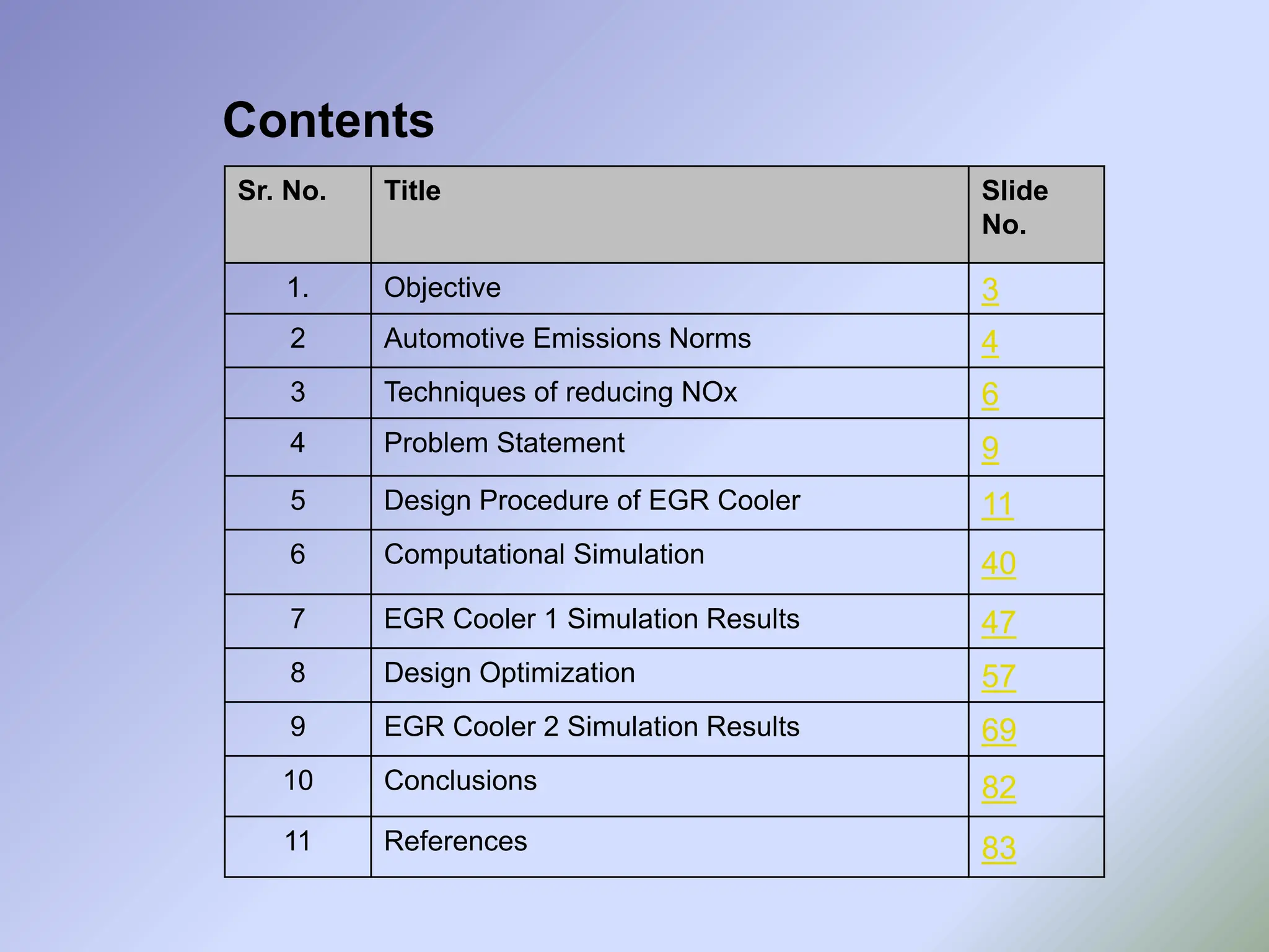
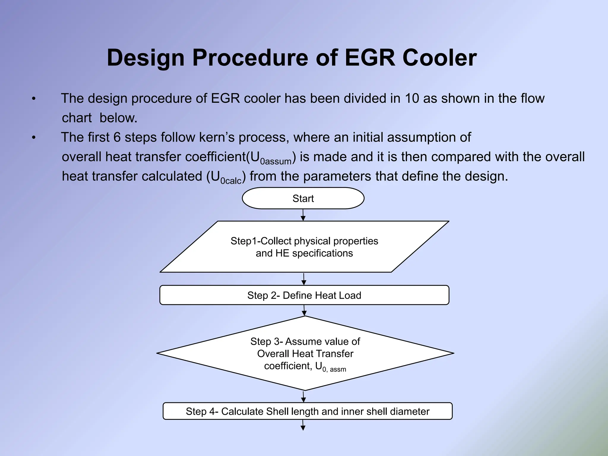
The document outlines the design and simulation of an exhaust gas recirculation (EGR) cooler aimed at reducing nitrogen oxide (NOx) emissions in automotive applications. It details the design process, input parameters, and computational methods used to achieve effective cooling of recirculated exhaust gases as mandated by stringent automotive emission norms in India. The study emphasizes the necessity for a high-performance EGR cooler and discusses various techniques for NOx reduction across different stages of combustion.

1. Design and Simulation of EGR Cooler
Aditya Bharat Patil
M.Tech Automotive (ARAI-VIT Vellore)
B.E. Mechanical (MAE, Alandi, Pune)

2. Sr. No. Title Slide
No.
1. Objective 3
2 Automotive Emissions Norms 4
3 Techniques of reducing NOx 6
4 Problem Statement 9
5 Design Procedure of EGR Cooler 11
6 Computational Simulation 40
7 EGR Cooler 1 Simulation Results 47
8 Design Optimization 57
9 EGR Cooler 2 Simulation Results 69
10 Conclusions 82
11 References 83
Contents

3. • To design and validate an Exhaust Gas Recirculation (EGR) cooler so that
effective cooling of exhaust gas, that is recirculated to an engine in order to
reduce its NOx emissions, is achieved.
Objective

4. Automotive Emissions and Norms
• Bharat Stage emission norms are regulations put by Government of India
to control the air pollutants emitted by internal combustion engines
and motor vehicles [1] .
• These are implemented by Central Pollution Control Board (CPCB).
• These were first implemented in year 2000 in accordance with European Emission
norms.
• In year 2010 Bharat IV emission norms were implemented.
• As per the notification released by Government of India in February 2016, it has
been decided to skip Bharat V norms and move towards Bharat VI norms.
• Bharat VI norms will be implemented from April 2020.

5. Comparison Bharat IV, V, VI Norms
Stage CO
(g/km)
HC
(g/km)
HC+Nox
(g/km)
NOx
(g/km)
Gasoline Diesel Gasoline Diesel Gasoline Diesel Gasoline Diesel
BS IV 1 0.5 0.10 - - 0.3 0.08 0.25
BS V 1 0.5 0.10 - - 0.23 0.06 0.18
BS VI 1 0.5 0.10 - - 0.17 0.06 0.08
Table 1 [1]
*For passenger cars

6. Techniques Of Reducing NOx
• Techniques of reducing NOx can be categorized along the three different stages
of combustion as enlisted below.[2]
1. Pre-combustion:
Different ways to reduce NOx during pre-combustion are,
- Low Swirl
- Turbo Charger Intercooling
- Fuel Quality
2. During Combustion:
The methods that can be used during combustion to control NOx are,
- Injection
- Combustion chamber
- EGR
3. Post Combustion:
- Selective Non Catalytic Reduction (SNCR)
- Urea Selective Catalytic Reduction (SCR)
- Lean NOx Trap (LNT)

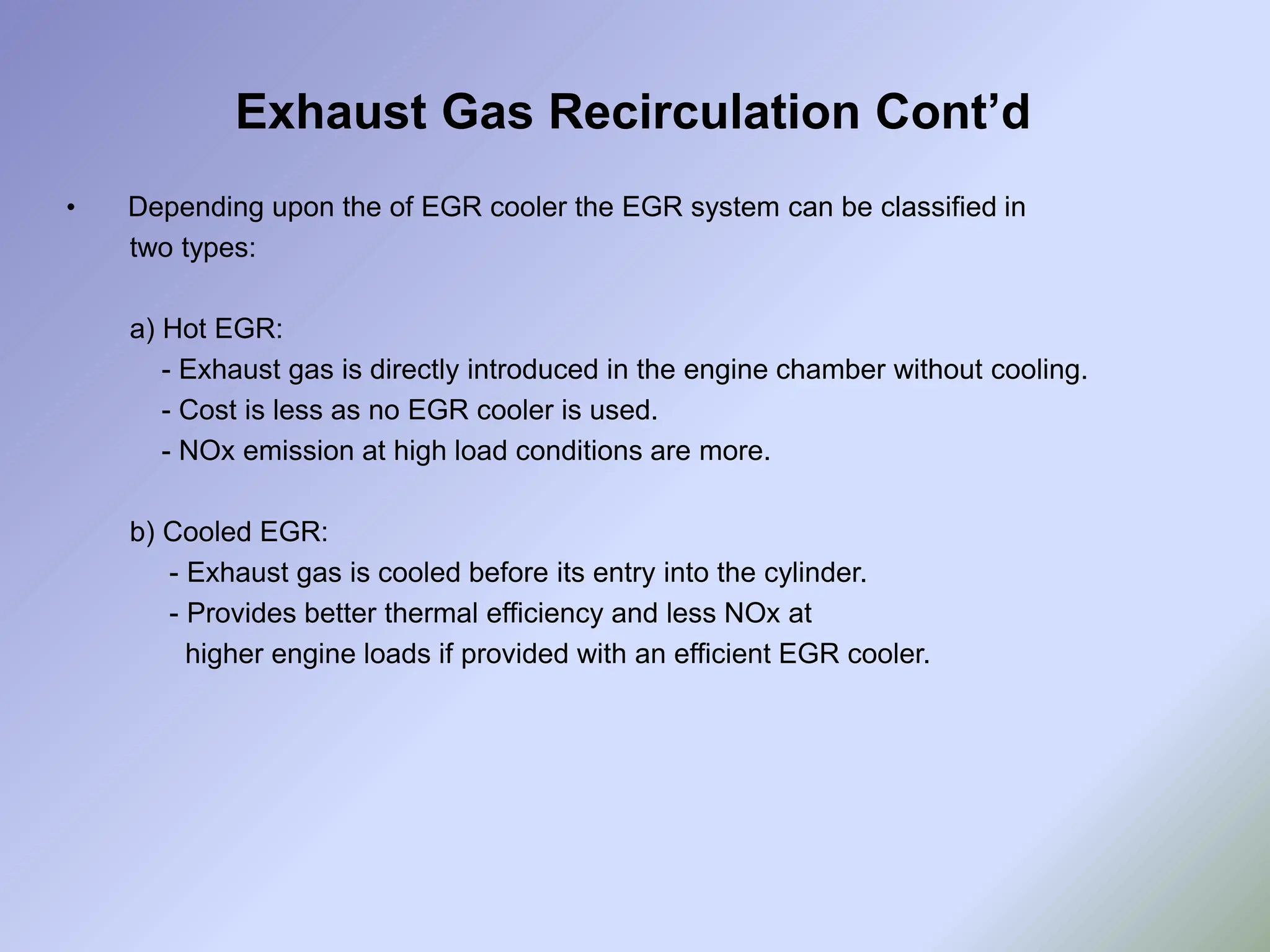
7. Exhaust Gas Recirculation
• EGR lowers the combustion temperature which in turn lowers the NOx,
by diluting the mixture in the heat cylinder and absorbing heat from burning fuel.
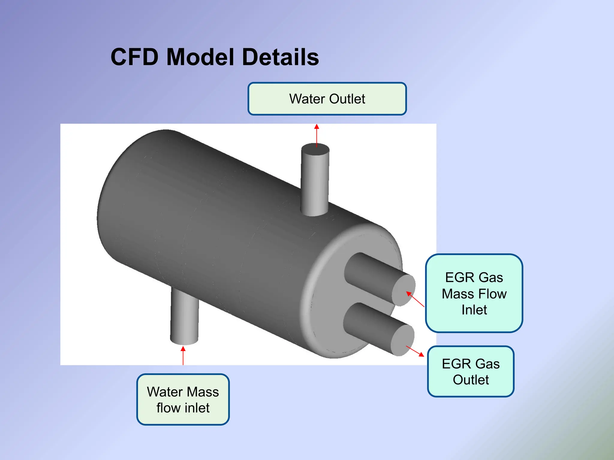
• The various components of EGR system are shown in figure below.
Figure No. 1 [3]

8. Exhaust Gas Recirculation Cont’d
• Depending upon the of EGR cooler the EGR system can be classified in
two types:
a) Hot EGR:
- Exhaust gas is directly introduced in the engine chamber without cooling.
- Cost is less as no EGR cooler is used.
- NOx emission at high load conditions are more.
b) Cooled EGR:
- Exhaust gas is cooled before its entry into the cylinder.
- Provides better thermal efficiency and less NOx at
higher engine loads if provided with an efficient EGR cooler.

9. Problem Statement
• Due drastic climate changes taking place in recent years and increased
awareness about the hazards of environmental pollution, efforts are been
made all over world to reduce pollution.
• As a result of this all the industrial sectors are subjected to stringent emission
norms, and so is the automotive sector.
• Nitrogen Oxides (NOx), is one of the various emissions from exhaust
system of automobiles that needs to be controlled.
• One of the various available methods to reduce NOx is use of Exhaust Gas
Recirculation (EGR) system.
• For efficient working of an EGR system a high performance EGR cooler is must.
The purpose of this project is to design an EGR cooler that gives essential
temperature drop as per desired from the given input data.

10. Input and Desired Output Data
Sr. No. Parameter Value
1. Exhaust gas inlet Temp T1 (K) 773
2. Water inlet Temp. t1 (K) 358
3. Exhaust gas mass flow rate (kg/hr) 50
Table 2
Sr. No. Parameter Value
1. Exhaust gas outlet Temp. T2 (K) 423
2. Water outlet Temp. t2 (K) 371
Table 3
Given Input :
Desired Output :

11. Design Procedure of EGR Cooler
• The design procedure of EGR cooler has been divided in 10 as shown in the flow
chart below.
• The first 6 steps follow kern’s process, where an initial assumption of
overall heat transfer coefficient(U0assum) is made and it is then compared with the overall
heat transfer calculated (U0calc) from the parameters that define the design.
Start
Step 2- Define Heat Load
Step1-Collect physical properties
and HE specifications
Step 3- Assume value of
Overall Heat Transfer
coefficient, U0, assm
Step 4- Calculate Shell length and inner shell diameter

12. Design Procedure of EGR Cooler Cont’d
Step 5- Estimate heat transfer coefficient
Step 6- Overall Heat Transfer coefficient calculation
Step 7- Shell Diameter and Thickness
Step 8- Shell Front and End Cover
Step 9- Design of front end tube sheet
Step 10- Design Of rear End Tube Sheet
End
Figure No. 2

13. Step 1- Collect Physical Properties and HE
Specifications
• Physical Properties:
• HE Specifications:
- Exhaust Gas is corrosive so we are assigning it to tube side.
- Using one shell pass and two tube passes
- Shell side fluid is cooling water, which is much cleaner. So considering triangular
pitch to minimize the volume of HE(pitch is the distance between centers of two tube).
Sr. No. Property Exhaust Gas
(HOT air at 800K)
Water
1. Viscosity (Pa-sec) X 10-3 0.0374 0.315
2. Density (kg/m3 ) 0.435 1000
3. Thermal Conductivity (W/m-K) 0.0577 0.6753
4. Specific Heat Capacity (KJ/Kg.K) 1.063 4.187
5. Specific gravity 0.435 * 10-3 1
6. Fouling Factor of exhaust 0.00176 0.00018
Table 4 [4]

14. Tube Arrangements
 Different types of tube arrangements triangular, rotated triangular, square and rotated
square are shown below (Figure No.3)
 A square, or rotated square arrangement, is used for heavily fouling fluids, where it is
necessary to mechanically clean the outside of the tubes, as the shell side fluid is water in
this case, selection of rotated triangular (Refer Fig. No 3) pattern is optimum.
 As per recommended by the TEMA( Tubular Exchanger Manufacturer’s Association) for
triangular arrangement of tubes pitch should be 1.25 times the outer diameter of the tube.
Figure No.3 [5]

15. • To start step 2, the heat transfer rate of exhaust gas needs to be calculated.
• Heat Load = 50*1.063*(773-423)/3600 = 5.17 kW
• Cold and hot stream heat loads are equal hence the flow rate of cold water is
calculated as:
Cooling flow water rate : = (5.17/(4.187*13)) =0.095 Kg/sec
• Logarithmic Mean Temperature Difference (LMTD):
LMTD =
T1
−t2
−(T2
−t1
)
ln
(T1
−t2
)
(T2
−t1
)
=
(773−371)−(423−358)
ln
(773−423)
(423−358)
= 184.96
Step 2- Define Heat Load
 
2
1
*
* T
T
C
m
Q h
h 

)
(
* 1
2 t
t
C
Q
m
c
c



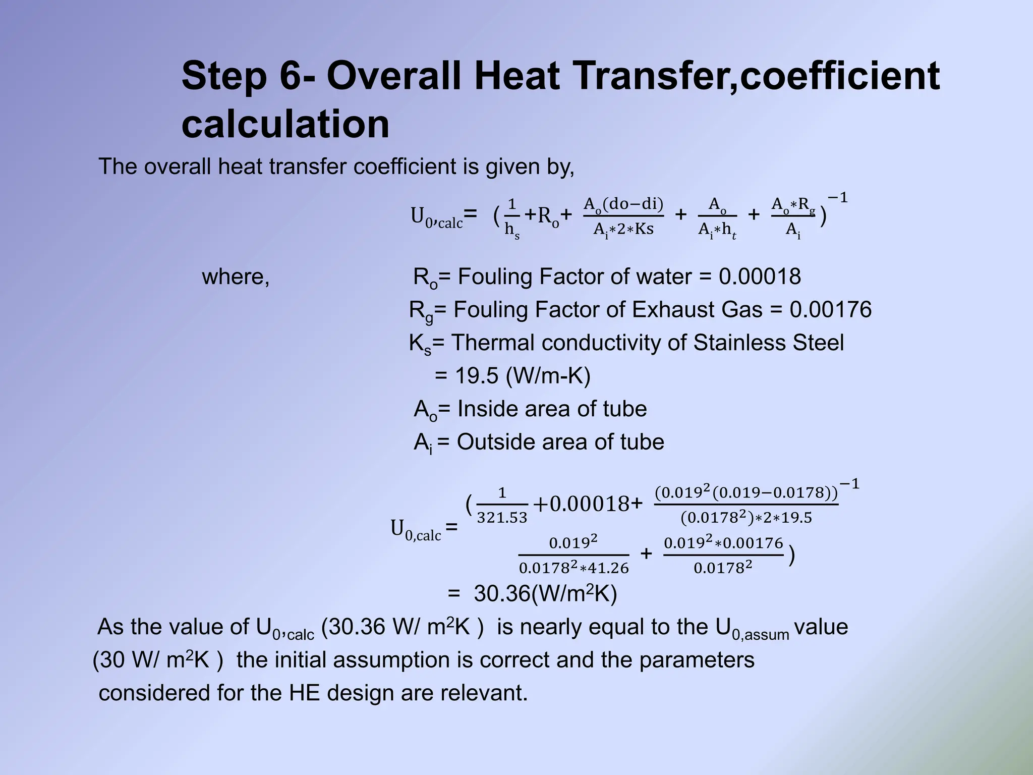
16. Step 3- Assume value of overall heat
transfer coefficient U0, assm
• Typical values of the overall heat-
transfer coefficient for various types of
heat exchanger are given in Figure 4.
• Figure No.4 can be used to estimate the
overall coefficient for tubular exchangers
(shell and tube).
• The film coefficients given in Figure No.
4 include an allowance for fouling.
• From Figure No.4 we take
U= 30 W/m2K
Figure No. 4 [6]

17. Step 4 - Calculate length of shell
and inner shell diameter
• Area= (
Q
U∗LMTD
) = (
5.167∗1000
30∗184.96
)= 0.93 m2
• Choose 19.05 mm (0.75 inch) outside diameter(do), 17.8 mm
inside diameter (di), 15 number of tubes (N), stainless steel
• Thus, the length (L) of tubes can be calculated as,
L= (
A
π∗do∗N
) = (
0.93
π∗0.019∗15
) = 1.07m
• As we have two number of passes the actual length of the
tube will be,
(L/2) = 0.535m
• An estimate of the bundle diameter Db can be obtained from
an equation, which is an empirical equation based on standard
tube layouts.
Figure No. 5
di=17.80 mm
do=19.05 mm
Figure No. 6
L= 535 mm

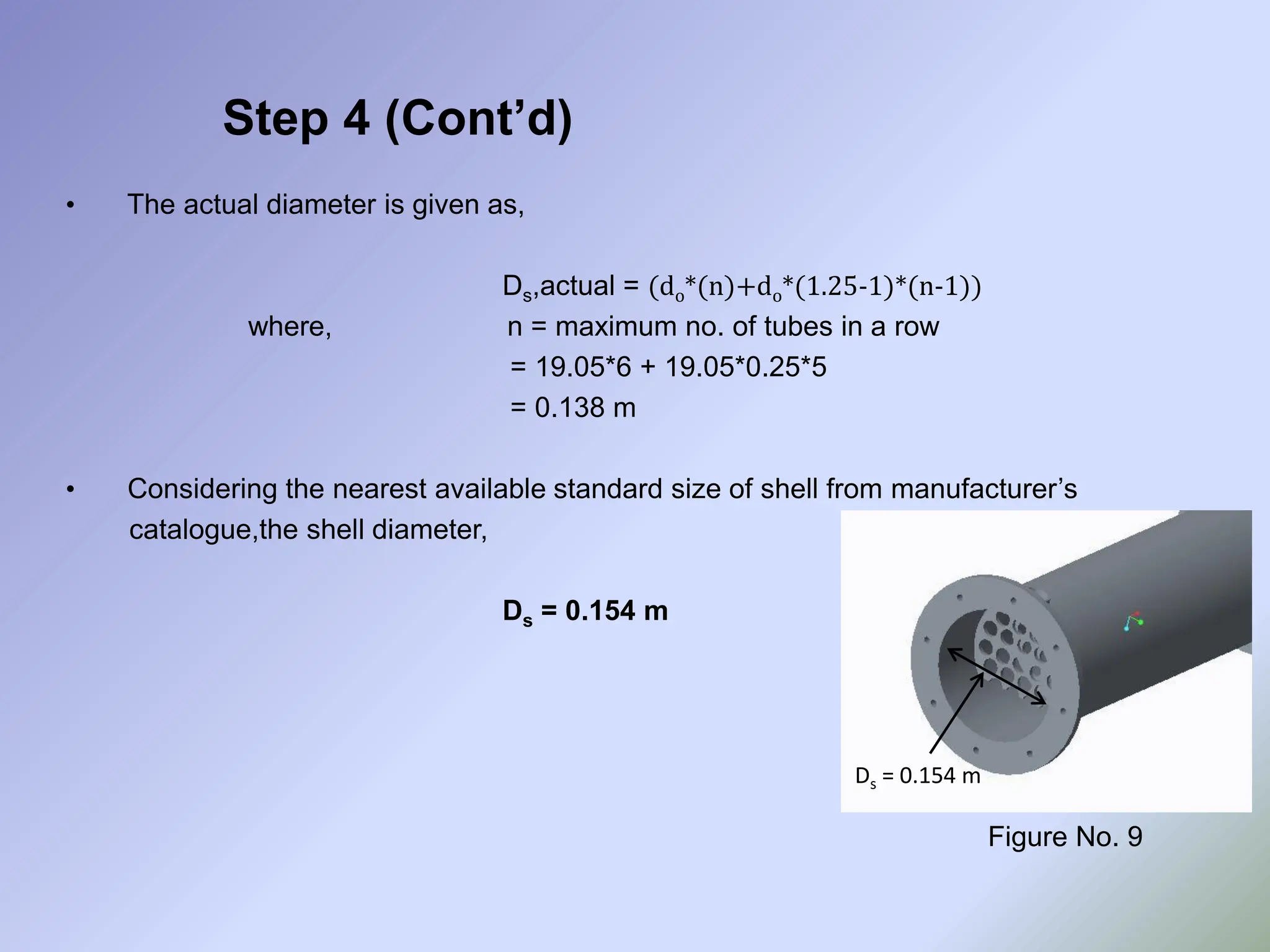
18. Step 4 (Cont’d)
• The constants for use in this equation, for triangular and square patterns,
are given in Figure No. 7.
Db= (do* (
N
K1
)(
1
n
)
)
where Db= bundle diameter in mm, do = tube outside diameter in mm.,
N = number of tubes
• So, in our case we have:
Db= (0.019* (
15
0.249
)(
1
2.201
)
) = 0.122 m.
Figure No.7 [7]

19. Step 4 (Cont’d)
• Figure No.8 gives the graph from
where the bundle diameter can
be estimated for different types of
head.
• Shell diameter (Ds):
Ds = (Bundle diameter + Clearance)
= 0.122 + 0.0061
= 0.128 mm
• The actual bundle diameter, that
has been calculated by the
arrangement of tubes varies with that
of obtained from formula above.
Figure No. 8 [7]

20. Step 4 (Cont’d)
• The actual diameter is given as,
Ds,actual = (do*(n)+do*(1.25-1)*(n-1))
where, n = maximum no. of tubes in a row
= 19.05*6 + 19.05*0.25*5
= 0.138 m
• Considering the nearest available standard size of shell from manufacturer’s
catalogue,the shell diameter,
Ds = 0.154 m
Figure No. 9
Ds = 0.154 m

21. Step 5- Estimate heat transfer coefficient
• Tube Side Heat transfer Coefficient:
a) Tube side velocity,(velocity of exhaust gas) ut:
Mass flow rate of exhaust gas,
mh= Density of gas*Area available
for flow*Velocity of gas
ut= (
(number of passes/number of tubes)∗mh
Density of gas∗Area available for flow
)
= (
4∗(50/3600)∗(2/15)
0.435∗∏∗0.0178∗0.0178
)
ut = 18.34 m/sec.
b) Tube Side Reynolds's Number, Re:
Re = (
Density of gas∗Velocity of gas∗di
Viscosity of Exhaust gas
)
Re = (
0.435∗18.34∗0.0178
0.0000374
)
Re = 3796.96

22. Step 5 (Cont’d)
c) Tube Side Prandtl number, Pr:
Pr= (
Viscosity of Exhaust gas∗Specific heat of exhaust gas
Thermal Conductivity of Exhaust gas
)
Pr= (
µ∗Ch
𝐾
)
= (
0.0000374∗1.063∗1000
0.0577
)
= 0.689
d) Tube Side Nusselt number, Nu:
As the Reynolds's number is in range between 3000<Re< 5*106,
we will use Gnielinski corelation,
Nu = {
f
8
∗ Re−1000 ∗Pr
1+12.7∗
f
8
1
2
∗(Pr
(
2
3)
)
}
where f is Darcy friction factor and is given as,
f = (0.79 ln(Re) −1.64)−2
= (0.79 ln(3796.96) −1.64)−2
= 0.04214

23. Step 5 (Cont’d)
Nu = {
0.04214
8
∗(3796.96−1000)∗0.689
1+12.7∗
0.04214
8
1
2
∗(0.689
(
2
3)
)
} = 12.7
e) Tube Side Heat Transfer Coefficient:
The Nusselt number is given as,
Nu = (
ht∗Lc
K
)
where, ht= heat transfer coefficient for tube side, (W/m2.K)
Lc= characteristic length, (mm) ( inner diameter
of tube di, in our case)
K = thermal conductivity of exhaust gas (W/m-K)
Thus,
ht = (
Nu∗K
Lc
)
= (
12.73∗0.0577
0.0178
)
ht = 41.26 (W/m2.K)
ht
Figure No. 10

24. Step 5 (Cont’d)
• Shell Side Heat Transfer Coefficient:
a) Baffles:
The baffle spacing used is range from 0.2 to 1.0 shell diameters.
A close baffle spacing will give higher heat transfer coefficients
but at the expense of higher pressure drop.
Considering baffle spacing = ( 0.5*Ds )= (0.5*0.154) = 0.077m
From literature survey, 25% cut baffles gives lesser flow reversal and higher heat
transfer coefficient, considering the same here.
Thus the number of baffles required will be,
Bn= (
Length of tubes
Baffle Spacing
) = (
0.535
0.077
) = 6.74 ~ 7
Baffle
Figure No. 11

25. Step 5 (Cont’d)
b) Shell Equivalent Diameter (Hydraulic Diameter):
De=(
(
𝑝𝑡
2
∗0.87∗𝑝𝑡−0.5∗π∗𝑑𝑜
2
(π∗
𝑑𝑜
2
)
) = (
1.10(𝑝𝑡
2−0.917∗𝑑𝑜
2
𝑑𝑜
)
where, pt is tube pitch,
pt= (1.25*19.05) = 23.81 mm
De= (
1.10(0.023812−0.917∗0.0192
0.019
) m
= 0.0137 m
c) Cross Flow Area (As) for water along shell side:
As= (
Tube Clearance ∗Baffle Spacing∗Shell inner diameter
Tube Pitch
)
= (
0.023−0.019 ∗0.077∗0.154
0.023
)
= 0.00206 m2

26. Step 5 (Cont’d)
d) Shell Side Mass Velocity:
Us = (
Mass Flow rate of water
Cross Flow area for water
)
Us= (
0.095
0,00206
) = 46.1165
e) Shell Side Reynolds’s Number, Res:
Res= (
Density of water∗Velocity of water∗De
Viscosity of water
)
= (
1000∗46.1165∗0.0137
0.315
) = 2005.7017
f) Shell Side Prandtl Number, Prs:
Prs= (
Viscosity of Exhaust gas∗Specific heat of water
Thermal Conductivity of Water
)

27. Step 5 (Cont’d)
Prs= (
µ∗Cc
𝐾
) = (
4.187∗1000∗0.315
0.6735
) = 1.953
g) Shell side Nusselt Number, Nus:
Using Sieder-Tate equation as the flow is laminar,
Nus=(1.86*Res(
1
3
)
*Prs(
1
3
)
*
De
L
(
1
3
)
)
Nus=(1.86*2005.70(
1
3
)
*1.953(
1
3
) 0.0137
1.038
(
1
3
)
)
Nus = 6.5208
h) Shell side heat transfer coefficient:
Nus= (
hs
∗Lc
K
)
hs= (
Nus
∗K
Lc
)
= 321.5337 (W/m2.K)
Figure No.12
hs

28. Step 6- Overall Heat Transfer,coefficient
calculation
The overall heat transfer coefficient is given by,
U0,calc= (
1
hs
+Ro+
Ao(do−di)
Ai∗2∗Ks
+
Ao
Ai∗h𝑡
+
Ao∗Rg
Ai
)
−1
where, Ro= Fouling Factor of water = 0.00018
Rg= Fouling Factor of Exhaust Gas = 0.00176
Ks= Thermal conductivity of Stainless Steel
= 19.5 (W/m-K)
Ao= Inside area of tube
Ai = Outside area of tube
U0,calc =
(
1
321.53
+0.00018+
(0.0192(0.019−0.0178))
(0.01782)∗2∗19.5
0.0192
0.01782∗41.26
+
0.0192∗0.00176
0.01782 )
−1
= 30.36(W/m2K)
As the value of U0,calc (30.36 W/ m2K ) is nearly equal to the U0,assum value
(30 W/ m2K ) the initial assumption is correct and the parameters
considered for the HE design are relevant.

29. Step 7- Shell Diameter and Thickness
• The shell thickness (ts), can be calculated from the equation below based
on the maximum allowable stress and corrected for the joint efficiency,
ts= (
p∗Ds
fJ−0.6∗p
+ c)
where, ts= shell thickness, mm
p = design pressure, Pa.
• Exhaust gas pressure in diesel engine lies in the range of 1.5 – 2 bar.
• As it is case of steady flow of energy for cooling water, the pressure of cooling
water is considered as 1 bar. Thus the maximum pressure may be around
2 bar approximately in EGR cooler.
• The shell has been designed for 9 bar which nearly 5 times the maximum pressure.

30. Step 7 Cont’d
Ds= shell ID =0.154 m
f = maximum allowable stress of the material
construction (stainless steel 304L)
= 90 MPa.
c = corrosion allowance
= 0.063inch ( for stainless steel 304L)
= 1.6002 mm
J = joint efficiency
= 0.8 (for bolted joints)
Thus,
ts=
9∗105∗0.154
90∗106∗0.8−0.69∗9∗105+ 0.0016002
= 0.00354 m = 3.54 mm.
• Considering fouling due water, the shell thickness is taken as 5mm.

31. Step 7 Cont’d
• Now, the shell outer diameter can be given
as,
Do = Ds + 2* ts
= 0.154 + 2*0.005
Do = 0.164m
The overall dimensions of the shell are
enlisted in table 5 below.
Sr.No. Parameter Value (m)
1. Inner Diameter 0.154
2. Outer Diameter 0.164
3. Length 0.535
4. Flange Diameter 0.230
5. Flange Thickness 0.010
Table 5
Figure No.13
Figure No.14
Do = 0.164m
Df = 230 mm

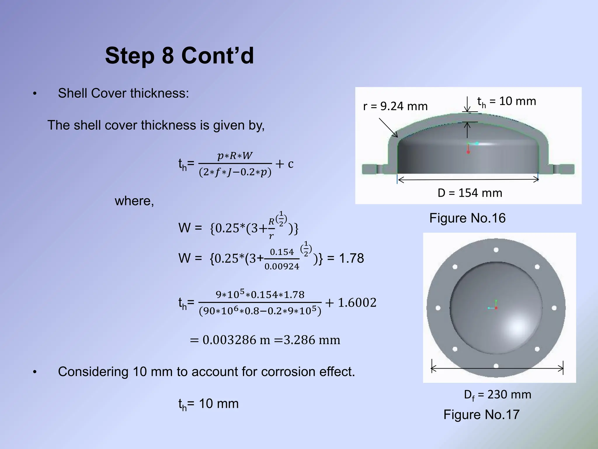
32. Step 8- Front and End Cover
• Different types of shell covers such as flat, torispherical, hemispherical,
conical and ellipsoidal are used in shell and tube type of heat exchangers.
• Torispherical type is commonly used in chemical industries. Figure 15 shows the
various dimensions in it. We are considering the same in this case.
R = crown radius = Ds = 0.154 m
r = knuckle radius= (0.06*R)=0.00924 m
Hi= inside depth of head
= (R – {(R−
𝐷𝑠
2
) ∗ (R+
𝐷𝑠
2
) + 2∗r}(
1
2
)
)
= (154 – {(154−
154
2
) ∗ (154+
154
2
) + 2∗9.24}(
1
2
)
)
= 20.56 mm
Figure No. 15 [8]

33. Step 8 Cont’d
• Shell Cover thickness:
The shell cover thickness is given by,
th=
𝑝∗𝑅∗𝑊
(2∗𝑓∗𝐽−0.2∗𝑝)
+ c
where,
W = {0.25*(3+
𝑅
𝑟
(
1
2
)
)}
W = {0.25*(3+
0.154
0.00924
(
1
2
)
)} = 1.78
th=
9∗105∗0.154∗1.78
(90∗106∗0.8−0.2∗9∗105)
+ 1.6002
= 0.003286 m =3.286 mm
• Considering 10 mm to account for corrosion effect.
th= 10 mm
Figure No.16
Figure No.17
D = 154 mm
r = 9.24 mm th = 10 mm
Df = 230 mm

34. Step 8 Cont’d
 Design Features of Front End Shell Cover:
• All features are same as Rear End Shell
cover in addition the depth of the cover has
been increased to 60 mm instead of 20 mm
(like in rear end cover). Also a partition (pc) of
5 mm thick has been provided over the
whole depth to avoid mixing of incoming
and outgoing gas.
Sr. No. Parameter Value (mm)
1. Knuckle Radius 9.24
2. Inside Depth 20
3. Thickness 10
4. Flange Diameter 230
5. Flange Thickness 10 Figure No.19
Figure No.18
Table 6
Df = 230 mm
pc = 5 mm

35. Step 9- Design Of Front End Tube Sheet
Sr. No. Parameter Value
(m)
1. Diameter 0.230
2. Thickness 0.020
3. Diameter of Tube Holes 0.01905
4. Tube Pitch 0.02381
Table 7
Figure No.20
Figure No.21
Dt = 230 mm
pt= 23.81 mm
do = 19.05 mm
st = 20 mm

36. Step 10- Design of Rear End Tube Sheet
• The design parameters of the end tube
sheet are enlisted in table below.
• Almost all the dimensions are same as that
of the front end tube sheet, except an extra
rib of 3mm thickness ,20 mm width and
its length equal to inner diameter of shell
has been added to guide the flow of gas.
Sr. No. Parameter Value (m)
1. Diameter 0.230
2. Thickness 0.020
3. Rib Thickness 0.003
4. Rib Width 0.020
5. Rib Length 0.154
Figure No.23
Figure No.22
Table 8
rw = 20 mm
rt = 3 mm
rl= 154 mm

37. CAD Model of Tubes
 Selection of tubes was done to validate the
initial approximation of the overall heat
transfer coefficients.
The table below shows all the parameters
the tubes.
Sr. No. Parameter Value
1. Inner Diameter 0.0178 (m)
2. Outer Diameter 0.01905 (m)
3. Tube Pitch 0.02381 (m)
4. Length of tubes 0.535 (m)
5. Number Of tubes 15
Figure No.24
Figure No. 25
Table 9
pt= 23.81 mm

38. Overall length Of EGR Cooler
• Thus after designing all the parts the overall
length of the EGR Cooler can be given as,
𝐿𝑜= Length of Front end Cover (Lfc)
+Length of Front end Tube Sheet(Lfs)
+Length of Shell (Ls)
+Length of Rear end Tube Sheet( Lrs)
+Length of Rear end Cover (Lrc)
= 0.535 + 0.020 + 0.020 + 0.10611+
0.066
= 0.74711 𝑚
𝐿𝑜 = 0.748 𝑚.
Figure No.26
Figure No.27
Ls
Lfc
Lfs Lrs Lrc

39. EGR Cooler Specifications
Sr. No. Parameter Value
1. Length (Lo) 0.748 (m)
2. Width (W) 0.23 (m)
3. Height (H) 0.23 (m)
4. Material Stainless Steel
5. Type Shell and Tube HE
6. Number of Passes 2
7. Number of Tubes 15
8. Type of tubes Full smooth
9. Shell ID 0.154 (m) Figure No.29
Figure No.28
Table 10
Lo
W
H

40. EGR Cooler 1 CFD Mesh
15.5 million cells
Water and exhaust gas (Air )
domains along with steel tubes are
meshed with mixed type of elements
consisting of tetrahedral, triangular
and quadrilateral elements

41. EGR Cooler 1 CFD Mesh Cont’d
0.65 million cells 0.65 million cells
GAS Tubes WATER Tubes
Stainless steel tubes are divided in
two parts, water tubes (for outer
diameter) and gas tubes (for inner
diameter) and are meshed with
mixed type of elements consisting
of tetrahedral, triangular and
quadrilateral elements

42. CFD Model Details
Water
Outlet
Water Mass
flow inlet
EGR Gas
Outlet
EGR Gas
Mass Flow
Inlet
Here for exhaust gas(air) ,
integrated inlet and outlet
conditions are defined which will
automatically set the distribution of
the mass through the pipes.
Outer walls

43. Assumptions made during CFD simulations of EGR cooler are enlisted below:
1. Radiative heat transfer has not been considered.
2. The outer wall of EGR cooler is considered to be adiabatic ( no heat transfer either by
convection or by radiation will take place through it).
3. Exhaust gas (air) follows ideal gas equation of state (PV = mRT).
4. The properties of both fluids (neither water nor air) do not change with temperature. This
assumption has to be validated as it may introduce significant error in results.
CFD Model Assumptions

44. Material Properties
Property Water
(Fluid 1)
Exhaust Gas
(Air)
(Fluid 2)
Stainless
Steel
(Solid)
Dynamic Viscosity kg/m.s) X 10-3 0.001 1.78E-05 NA
Density (kg/m3 ) 998.2 As per ideal gas
equation
8030
Thermal Conductivity (W/m-K) 0.6 0.0242 16.27
Specific Heat Capacity (KJ/kg.K) 4.182 1.003 0.502
Table 11

45. CFD domain consists of 3 regions mentioned below:
1. Exhaust Gas (Hot Air)
2. Water
3. Solid for steel pipes
The boundary conditions for respective regions are as follows:
CFD Model – Boundary Conditions
Water Inlet:
Mass Flow Rate = 0.0943 kg/sec
Temperature = 358 K (85 ° c )
Water Outlet : Outlet
Exhaust Gas (Air) Inlet:
Mass Flow Rate = 0.01388kg/sec
Temperature = 773 K (500 ° c )
Exhaust Gas (Air) Outlet : Outlet
Pipe Walls : Gas tubes and water tubes are modeled as conducting walls.
Outer walls : These are the outer walls of the water and gas region where velocities are
zero (no slip) and there is no heat transfer (adiabatic).
Turbulence model : k-Ɛ

46. Results: Static Pressure Contours
• The pressure contours
are shown over the
entire CFD domain.
• Maximum pressure is
seen at the entry of
EGR gas shown by
yellowish colour
contour(value 6.50
e+02) and then it is
seen when the flow
reversal takes place.
Water
In
Water
Out
EGR
Gas In
EGR Gas
Out
Area where Flow
reversal takes place

47. Results: Temperature Contours
• The temperature
contours are shown
over the entire CFD
domain.
• The drop in
temperature of
exhaust gas is seen
clearly.
The colour contour at the exhaust gas outlet temperature
shows that required cooling of exhaust gas is achieved.

48. Results : Temperature Contours Water
Tubes
• The temperature
contours are shown over
the tubes.
• The values are from the
water side of the tubes.

49. Results : Temperature Contours Gas
Tubes
• The temperature
contours are shown over
the tubes.
• The values are from the
gas side of the tubes.
High temperature
regions for the tubes,
which give us idea
about the areas prone
to failure due to high
temperature.

50. Results: Pressure Contours (y - section)
The contours plots are shown over the sections passing longitudinally through
the EGR. Pressure drop is clearly visible for the exhaust gas (air).
High pressure region is
seen in this region due
high velocity that can be
seen from slide no. 50

51. Results: Velocity Contours (y - section)
The contours plots are shown over the sections passing longitudinally through
the EGR.
High velocity of gas can
be seen here, and then
the velocity reduces due
to impact with wall in
front

52. Results: Temperature Contours(y-section)
• The contours plots are shown over the sections passing longitudinally
through the EGR.
• The minimum and maximum temperature in the EGR cooler can be seen
here.

53. Results: Temperature x-section
• The gradual drop in temperature over the entire CFD domain along X-section is
seen clearly.
• It is also clear that temperature for exhaust reaches it intermediate value when the
flow reversal takes place at reversing chamber.
Intermediate value
of temperature
during flow
reversal

54. Sr.No Parameter Analytical Simulation
1.
Exhaust Gas Outlet
Temperature (֯C)
150 151.34
2.
Water Outlet
Temperature (֯C)
98 97.8
Comparison Analytical and Simulation Results
Table 12
Effectiveness, e:
e = (
1−exp(−NTU∗(1−C))
1−C∗exp(−NTU∗(1−C))
) = (
1−exp(−1.94∗(1−0.03714))
1−C∗exp(−1.94∗(1−0.03714))
) = 0.8510

55. Sr. No. Parameter Model 1 Model 2 EGR Cooler 1
1. Length (mm) 162.8 104.60 748
2. Width (mm) 61 110 230
3. Height (mm) 118 149 230
Size Comparison
Table 13
Here,
Model 1 and Model 2 are the EGR Cooler models available in the market,
whereas EGR Cooler 1 is the model developed in house.

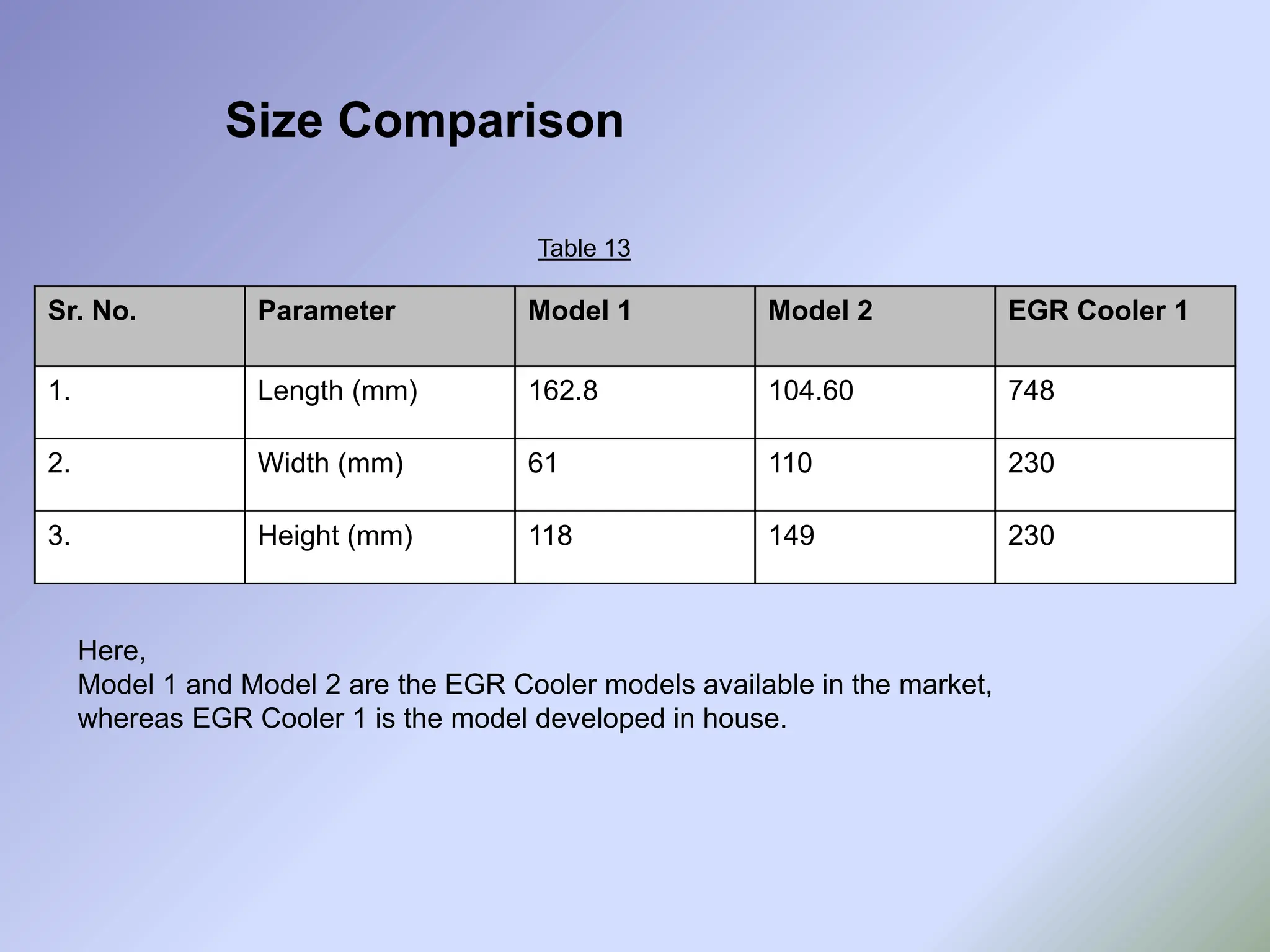
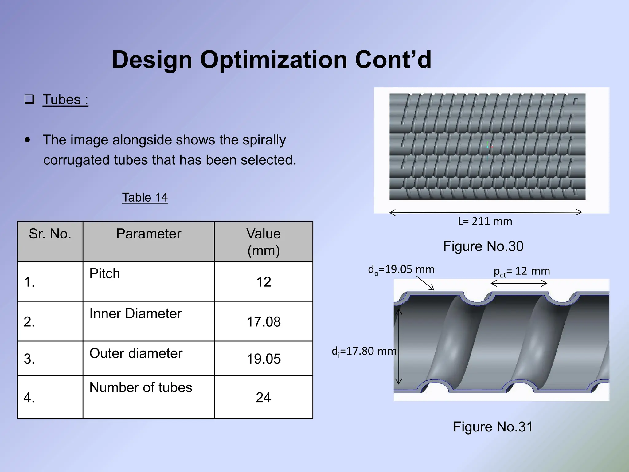
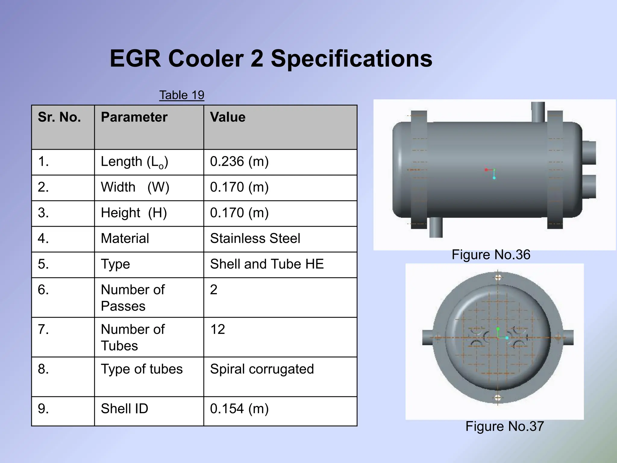
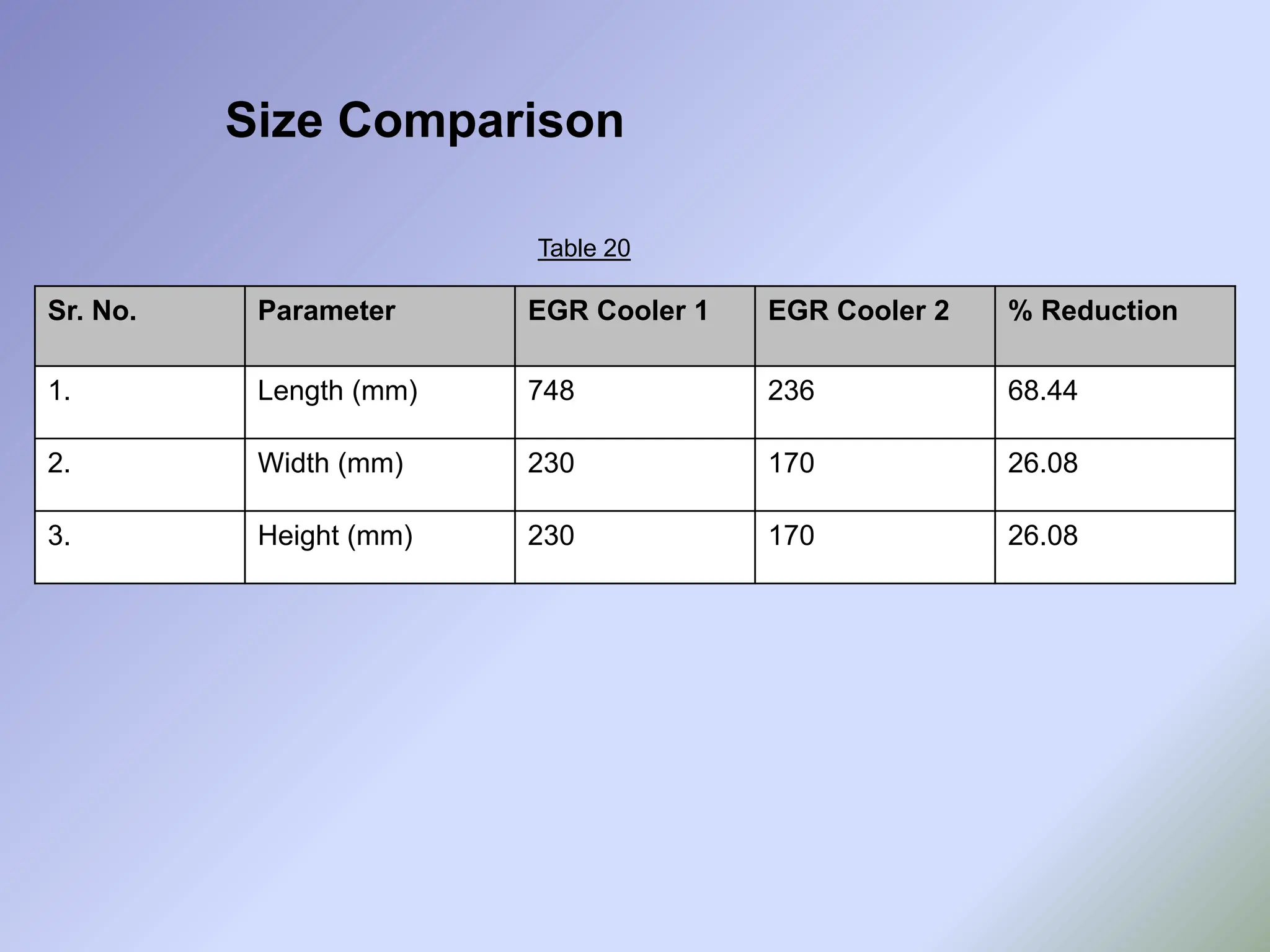
56. • As it can be seen from earlier slides, though the designed EGR cooler gives satisfactory
performance, its way too bigger in size than the available models in the market. Thus
the optimization of the design is must.
• Reducing the size of EGR cooler maintaining the same performance is a
challenging task.
• Earlier research work done in this field depicts that use of corrugated tubes increases the
heat transfer coefficient [13] .
• The new EGR cooler has been designed with corrugated tubes instead of fully smooth
tubes, relevant calculated required are mentioned in next slides.
Design Optimization

57.  Tubes :
 The image alongside shows the spirally
corrugated tubes that has been selected.
Sr. No. Parameter Value
(mm)
1.
Pitch
12
2.
Inner Diameter
17.08
3. Outer diameter 19.05
4.
Number of tubes
24
Table 14
Design Optimization Cont’d
Figure No.31
Figure No.30
di=17.80 mm
L= 211 mm
do=19.05 mm pct= 12 mm

58.  Reducing the number of tubes and implementation of spiral feature has increased the
various parameters on tube side, a comparison of these parameters for EGR Cooler 1
and EGR Cooler 2 is shown in table below.
Design Optimization Cont’d
Parameters EGR Cooler 1 EGR Cooler 2
Tube side velocity, ut 17.11619879 21.39524849
Reynolds Number, Ret 3543.602333 4429.502916
Prandtl Number, Prt 0.689015598 0.689015598
Nusselt Number, Nut 11.87782838 56.34426632
Convective heat transfer
coefficient, ht (W/m2/K)
38.50284816 182.6440543
Table 15

59. Design Optimization Cont’d
 Comparison of the shell side parameters for EGR Cooler 1 and EGR Cooler 2 is shown in
table below.
Parameters EGR Cooler 1 EGR Cooler 2
Cross flow area, as (m2) 0.002396499 0.001655601
Mass velocity , us 39.61369046 57.3412038
Reynolds Number, Res 1722.288687 2493.029694
jPrandtl Number, Prs 1.953065304 1.953065304
Nusselt Number, Nus 6.372549355 10.0555438
Convective heat transfer
coefficient, hs (W/m2/K)
314.22357 495.8280738
Table 16

60. Design Optimization Cont’d
The overall heat transfer coefficient is given by,
U0,calc= (
1
hs
+Ro+
Ao(do−di)
Ai∗2∗Ks
+
Ao
Ai∗h𝑡
+
Ao∗Rg
Ai
)
−1
where, Ro= Fouling Factor of water = 0.00018
Rg= Fouling Factor of Exhaust Gas = 0.00176
Ks= Thermal conductivity of Stainless Steel
= 19.5 (W/m-K)
Ao= Inside area of tube
Ai = Outside area of tube
U0,calc =
(
1
495.82
+0.00018+
(0.0192(0.019−0.0178))
(0.01782)∗2∗19.5
0.0192
0.01782∗182.64
+
0.0192∗0.00176
0.01782 )
−1
= 95.46(W/m2K)
As the value of U0,calc (95 W/ m2K ) is nearly equal to the U0,assum value
(95.46 W/ m2K ) the initial assumption is correct and the parameters
considered for the HE design are relevant.

61. Sr. No. Parameter Value
1. Length (Lo) 0.236 (m)
2. Width (W) 0.170 (m)
3. Height (H) 0.170 (m)
4. Material Stainless Steel
5. Type Shell and Tube HE
6. Number of
Passes
2
7. Number of
Tubes
12
8. Type of tubes Spiral corrugated
9. Shell ID 0.154 (m)
Table 19
EGR Cooler 2 Specifications
Figure No.36
Figure No.37

62. Sr. No. Parameter EGR Cooler 1 EGR Cooler 2 % Reduction
1. Length (mm) 748 236 68.44
2. Width (mm) 230 170 26.08
3. Height (mm) 230 170 26.08
Size Comparison
Table 20

63. EGR Cooler 2 CFD Mesh
31.1 million cells
Water and exhaust gas
(Air ) domains along
with steel tubes are
meshed with
tetrahedron elements

64. EGR Cooler 2 CFD Mesh Cont’d
GAS Tubes WATER Tubes
1.35million cells
1.47million cells
Stainless steel tubes are divide in
two parts, water tubes (for outer
diameter) and gas tubes (for inner
diameter) and are meshed wit h
tetrahedral elements.

65. CFD Model Details
Water Mass
flow inlet
Water Outlet
EGR Gas
Outlet
EGR Gas
Mass Flow
Inlet

66. Results: Static Pressure Contours
• The pressure contours
are shown over the entire
CFD domain

67. Results: Temperature Contours
• The temperature
contours are shown over
the entire CFD domain.
• The drop in temperature
of exhaust gas is seen
clearly.

68. Results : Temperature Contours Water
Tubes
• The temperature
contours are shown over
the tubes.
• The values are from the
water side of the tubes.

69. Results : Temperature Contours Gas
Tubes
• The temperature
contours are shown over
the tubes.
• The values are from the
gas side of the tubes.

70. Results: Pressure Contours (z - section)
• The contours plots for pressure are shown over the section passing through the
lateral plane located exactly at the centre of EGR.
• Pressure drop over entire CFD domain can be seen.

71. Results: Velocity Contours (z - section)
• The contours plots for velocity are shown over the section passing through the
lateral plane located exactly at the centre of EGR.
• Magnitude of velocity over entire CFD domain can be seen.

72. Results: Temperature Contours(z-section)
• The contours plots for temperatures are shown over the sections passing laterally
through the EGR.
• The variation in temperature along the lateral direction is seen clearly, it is also clear from
these contours that the temperature of exhaust gas is higher (168 ° c) than that required
(150 ° c)

73. Results: Temperature Contours(z-section)
• The contours plots for temperature are shown over the section passing through
the lateral plane located exactly at the centre of EGR.
• The temperature of exhaust gas at the outlet is higher than required is also
clearly visible.
Exhaust gas temperature
higher than that required

74. Results: Pressure x-section
• The gradual drop in pressure for exhaust gas (air) and water in the entire CFD
domain along X-section is seen clearly.
• The high pressure region of the exhaust gas (air) can also be seen clearly.
High pressure region for
exhaust gas
(air)

75. Results: Velocity x-section
• The gradual drop in velocity for exhaust gas (air) and water in the entire CFD
domain along X-section is seen clearly.
• The high velocity region of the exhaust gas (air) can also be seen clearly.
High velocity region for
exhaust gas
(air)

76. Results: Temperature x-section
• The drop in temperature for exhaust gas (air) in the entire CFD domain along X-section
is seen clearly.
• The high temperature region of the exhaust gas (air) can also be seen clearly,
that can help us know the region prone for failure due thermal stresses
High temperature region
for exhaust gas
(air)

77. Sr. No Parameter Analytical Simulation
1.
Exhaust Gas Outlet
Temperature (֯C)
150 168
2.
Water Outlet
Temperature (֯C)
98 96
Analytical vs Simulation Results
Table 21
Effectiveness, e:
e = (
1−exp(−NTU∗(1−C))
1−C∗exp(−NTU∗(1−C))
) = (
1−exp(−1.94∗(1−0.03714))
1−C∗exp(−1.94∗(1−0.03714))
) = 0.8510

78. Reasons for Deviation in Results
• The length of spiral tube required to
achieve the temperature is 211mm.
• The actual length in the model was
reduced to 199mm while
accommodating for the tube
sheets and for removing free
edges while meshing.
• A new design will be made (EGR
Cooler 3)with whole length of spirals
of 211mm and CFD analysis will be
done for that.
L= 211 mm
L= 199mm
Figure No.38

79. Conclusions
The following conclusions can be made from this project:
• An excel sheet based calculator has been developed that gives the
basic parameters in EGR cooler design tube dimensions, shell inner
diameter, length of tubes. It also gives an appropriate value of overall
heat transfer coefficient.
• Based on the inputs from excel sheet an EGR cooler model has been
developed for a specified range of exhaust gas temperature drop (350 ֯
C) and cooling water temperature rise (13 ֯ C). The CFD analysis of the
EGR cooler model gave satisfactory results with the temperature drop
on exhaust gas side deviating by 3.14% from the required result.
• The developed model is simple in design, manufacturable and
comparable in size with its market competitors.

80. References
1. Notification Draft, Central Motor Vehicles Amendment Rules (BHARAT VI),2015.
2. Automotive and Fuel Emissions Lecture Notes, ARAI Academy, 2017.
3. http://denso-europe.com/wp-content/uploads/2012/01/EGR-System2.jpg
4. S.S. Hoseini, G. Najafi , B. Ghobadian. Experimental and Numerical Investigation of
Heat transfer and turbulent characteristics of a EGR Cooler in Diesel Engine.
5. Lin Liu, Xiang Ling, Hao Peng. Analysis on flow and heat transfer characteristics of
EGR helical baffled cooler with spiral corrugated tubes.
6. E. Ozden, I. Tari. Shell side CFD analysis of a small shell-and-tube heat exchanger.
7. Eshita Pal,Inder Kumar, Jyeshtharaj B. Joshi, N.K. MahesCFD Simulations of shell-
side flow in a Shell and Tube heat Exchanger with and without Baffles.
8. http://www.engineeringtoolbox.com/air-properties-d_156
9. TEMA (8th Edition) Standards Of The Tubular Exchanger, Page 28,1999.
10. http://www.engineeringpage.com/technology/thermal/transfer.htm
11. Krishna Singh, Alen Soler. Mechanical Design of Heat Exchangers And Pressure
Vessel Components,1984.
12. http://c2109116.myzen.co.uk/wp-content/uploads/2013/03/torispherical_head-
1024x452.
13. S. Pethkool. “Turbulent heat transfer enhancement in a heat exchanger using helically
corrugated tubes.” 2011.

81. Thank You!