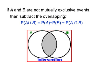
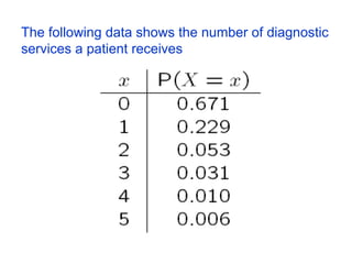
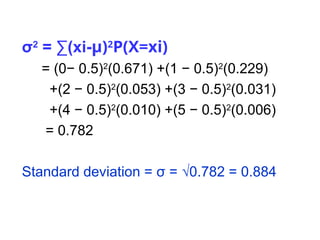
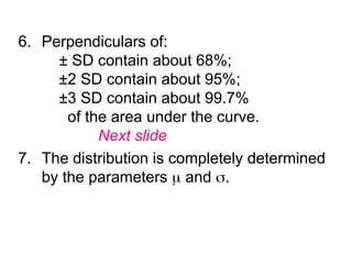
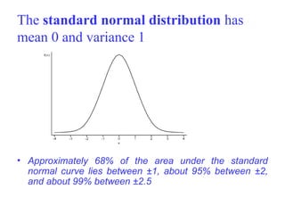
The document explains the fundamentals of probability and its distributions, highlighting its significance in both statistics and medicine. It covers concepts like objective and subjective probabilities, events, and the rules governing probability calculations, including independence and dependence of events. Additionally, it discusses the application of probability distributions in analyzing data and drawing conclusions from random variables.

1. Probability and Probability
Distributions

2. Probability
• Chance of observing a particular outcome
• Likelihood of an event
• Assumes a “stochastic” or “random”
process: i.e.. the outcome is not
predetermined - there is an element of
chance
• An outcome is a specific result of a single
trial of a probability experiment.

3. • Probability theory developed from the study
of games of chance like dice and cards.
• A process like flipping a coin, rolling a die or
drawing a card from a deck are probability
experiments.

4. Why Probability in Statistics?
• Results are not certain
• To evaluate how accurate our results are:
– Given how our data were collected, are our
results accurate ?
– Given the level of accuracy needed, how
many observations need to be collected ?

5. When can we talk about probability ?
• When dealing with a process that has an
uncertain outcome
• Experiment = any process with an uncertain
outcome
• When an experiment is performed, one and
only one outcome is obtained

6. • Event = something that may happen or not
when the experiment is performed
• An event either occurs or it does not occur
• Events are represented by uppercase
letters such as A, B, and C

7. • Probability of an Event E
= a number between 0 and 1 representing the
proportion of times that event E is expected to
happen when the experiment is done over and
over again under the same conditions
• Any event can be expressed as a subset
of the set of all possible outcomes (S)
S = set of all possible outcomes
P(S) = 1

8. Why Probability in Medicine?
• Because medicine is an inexact science,
physicians seldom predict an outcome with
absolute certainty.
• E.g., to formulate a diagnosis, a physician
must rely on available diagnostic information
about a patient
– History and physical examination
– Laboratory investigation, X-ray findings, ECG,
etc

9. • Although no test result is absolutely accurate, it
does affect the probability of the presence (or
absence) of a disease.
– Sensitivity and specificity
• An understanding of probability is fundamental
for quantifying the uncertainty that is inherent in
the decision-making process

10. • Probability theory is a foundation for
statistical inference, &
• Allows us to draw conclusions about a
population of patients based on
information obtained from a sample of
patients drawn from that population.

11. More importantly probability theory is used to
understand:
– About probability distributions: Binomial,
Poisson, and Normal Distributions
– Sampling and sampling distributions
– Estimation
– Hypothesis testing
– Advanced statistical analysis

12. Two Categories of Probability
• Objective and Subjective Probabilities.
• Objective probability
1) Classical probability and
2) Relative frequency probability.

13. Classical Probability
• Is based on gambling ideas
• Rolling a die -
– There are 6 possible outcomes:
– Total ways = {1, 2, 3, 4, 5, 6}.
• Each is equally likely
– P(i) = 1/6, i=1,2,...,6.
P(1) = 1/6
P(2) = 1/6
 …….
P(6) = 1/6
SUM = 1

14. • Definition: If an event can occur in N mutually
exclusive and equally likely ways, and if m of
these posses a characteristic, E, the probability
of the occurrence of E = m/N.
P(E)= the probability of E = P(E) = m/N
• If we toss a die, what is the probability of 4 coming
up?
m = 1(which is 4) and N = 6
The probability of 4 coming up is 1/6.

15. • Another “equally likely” setting is the
tossing of a coin –
– There are 2 possible outcomes in the set
of all possible outcomes {H, T}.
P(H) = 0.5
P(T) = 0.5
SUM = 1

16. Relative Frequency Probability
• In the long run process …..
• The proportion of times the event A occurs
— in a large number of trials repeated under
essentially identical conditions
• Definition: If a process is repeated a large
number of times (n), and if an event with the
characteristic E occurs m times, the relative
frequency of E,
Probability of E = P(E) = m/n.

17. • If you toss a coin 100 times and head
comes up 40 times,
P(H) = 40/100 = 0.4.
• If we toss a coin 10,000 times and the
head comes up 5562,
P(H) = 0.5562.
• Therefore, the longer the series and the longer
sample size, the closer the estimate to the true
value.

18. • Since trials cannot be repeated an infinite
number of times, theoretical probabilities are
often estimated by empirical probabilities
based on a finite amount of data
• Example:
Of 158 people who attended a dinner party,
99 were ill.
P (Illness) = 99/158 = 0.63 = 63%.

19. • In 1998, there were 2,500,000 registered live
births; of these, 200,000 were LBW infants.
• Therefore, the probability that a newborn is
LBW is estimated by
P (LBW) = 200,000/2,500,000
= 0.08

20. Subjective Probability
• Personalistic (represents one’s degree of belief
in the occurrence of an event).
• Personal assessment of which is more
effective to provide cure – traditional/modern
• Personal assessment of which sports team will
win a match.
• Also uses classical and relative frequency
methods to assess the likelihood of an event.

21. • E.g., If someone says that he is 95% certain
that a cure for AIDS will be discovered
within 5 years, then he means that:
P(discovery of cure for AIDS within 5 years)
= 95% = 0.95
• Although the subjective view of probability has
enjoyed increased attention over the years, it has not
fully accepted by scientists.

22. Mutually Exclusive Events
 Two events A and B are mutually exclusive if
they cannot both happen at the same time
P (A ∩ B) = 0
• Example:
– A coin toss cannot produce heads and tails
simultaneously.
– Weight of an individual can’t be classified
simultaneously as “underweight”, “normal”,
“overweight”

23. Independent Events
• Two events A and B are independent if the
probability of the first one happening is the
same no matter how the second one turns
out. OR. The outcome of one event has no effect on the
occurrence or non-occurrence of the other.
P(A∩B) = P(A) x P(B) (Independent events)
P(A∩B) ≠ P(A) x P(B) (Dependent events)
Example:
– The outcomes on the first and second coin
tosses are independent

24. Intersection, and union
• The intersection of two events A and B, A ∩ B,
is the event that A and B happen simultaneously
P ( A and B ) = P (A ∩ B )
• Let A represent the event that a randomly
selected newborn is LBW, and B the event that
he or she is from a multiple birth
• The intersection of A and B is the event that the
infant is both LBW and from a multiple birth

25. • The union of A and B, A U B, is the event
that either A happens or B happens or
they both happen simultaneously
P ( A or B ) = P ( A U B )
• In the example above, the union of A and
B is the event that the newborn is either
LBW or from a multiple birth, or both

26. Properties of Probability
1. The numerical value of a probability always
lies between 0 and 1, inclusive.
0  P(E)  1
 A value 0 means the event can not occur
 A value 1 means the event definitely will occur
 A value of 0.5 means that the probability that
the event will occur is the same as the
probability that it will not occur.

27. 2. The sum of the probabilities of all mutually
exclusive outcomes is equal to 1.
P(E1
) + P(E2
) + .... + P(En
) = 1.
3. For two mutually exclusive events A and B,
P(A or B ) = P(AUB)= P(A) + P(B).
If not mutually exclusive:
P(A or B) = P(A) + P(B) - P(A and B)

28. 4. The complement of an event A, denoted by
Ā or Ac
, is the event that A does not occur
• Consists of all the outcomes in which event
A does NOT occur
P(Ā) = P(not A) = 1 – P(A)
• Ā occurs only when A does not occur.
• These are complementary events.

29. • In the example, the complement of A is the
event that a newborn is not LBW
• In other words, A is the event that the child
weighs 2500 grams at birth
P(Ā) = 1 − P(A)
P(not low bwt) = 1 − P(low bwt)
= 1− 0.076
= 0.924

30. Basic Probability Rules
1. Addition rule
 If events A and B are mutually exclusive:
P(A or B) = P(A) + P(B)
P(A and B) = 0
 More generally:
P(A or B) = P(A) + P(B) - P(A and B)
P(event A or event B occurs or they both
occur)

31. Example: The probabilities below represent years of
schooling completed by mothers of newborn infants

32. • What is the probability that a mother has
completed < 12 years of schooling?
P( 8 years) = 0.056 and
P(9-11 years) = 0.159
• Since these two events are mutually
exclusive,
P( 8 or 9-11) = P( 8 U 9-11)
= P( 8) + P(9-11)
= 0.056+0.159
= 0.215

33. • What is the probability that a mother has
completed 12 or more years of schooling?
P(12) = P(12 or 13-15 or 16)
= P(12 U 13-15 U 16)
= P(12)+P(13-15)+P(16)
= 0.321+0.218+0.230
= 0.769

34. If A and B are not mutually exclusive events,
then subtract the overlapping:
P(AU B) = P(A)+P(B) − P(A ∩ B)

35. • The following data are the results of electrocardiograms
(ECGs) and radionuclide angiocardiograms (RAs) for 19
patients with post-traumatic myocardial confusions.
– 7 patients developed both ECG and RA abnormality
– 17 patients developed ECG abnormal
– 9 patients developed RA abnormal
P(ECG abnormal and RA abnormal) = 7/19 = 0.37
P(ECG abnormal or RA abnormal) =
P(ECG abnormal) + P(RA abnormal) – P(Both ECG and RA
abnormal) =
17/19 + 9/19 – 7/19 = 19/19 =1.
Note: The problem is that the 7 patients whose ECGs and RAs are both abnormal are counted twice

36. 2. Multiplication rule
– If A and B are independent events, then
P(A ∩ B) = P(A) × P(B)
– More generally,
P(A ∩ B) = P(A) P(B|A) = P(B) P(A|B)
P(A and B) denotes the probability that A and
B both occur at the same time.

37. Conditional Probability
• Refers to the probability of an event, given
that another event is known to have
occurred.
• “What happened first is assumed”
• Hint - When thinking about conditional probabilities, think in stages.
Think of the two events A and B occurring chronologically, one after
the other, either in time or space.

38. • The conditional probability that event B has
occurred given that event A has already
occurred is denoted P(B|A) and is defined
provided that P(A) ≠ 0.

39. Example:
A study investigating the effect of prolonged
exposure to bright light on retina damage in
premature infants.
Retinopathy
YES
Retinopathy
NO
TOTAL
Bright light
Reduced light
18
21
3
18
21
39
TOTAL 39 21 60

40. • The probability of developing retinopathy is:
P (Retinopathy) = No. of infants with retinopathy
Total No. of infants
= (18+21)/(21+39)
= 0.65

41. • We want to compare the probability of
retinopathy, given that the infant was
exposed to bright light, with that the infant
was exposed to reduced light.
• Exposure to bright light and exposure to
reduced light are conditioning events,
events we want to take into account when
calculating conditional probabilities.

42. • The conditional probability of retinopathy,
given exposure to bright light, is:
• P(Retinopathy/exposure to bright light) =
No. of infants with retinopathy exposed to bright light
No. of infants exposed to bright light
= 18/21 = 0.86

43. • P(Retinopathy/exposure to reduced light) =
# of infants with retinopathy exposed to reduced light
No. of infants exposed to reduced light
= 21/39 = 0.54
• The conditional probabilities suggest that premature infants
exposed to bright light have a higher risk of retinopathy than
premature infants exposed to reduced light.

44.  For independent events A and B
P(A/B) = P(A).
 For non-independent events A and B
P(A and B) = P(A/B) P(B)
(General Multiplication Rule)

45. Test for Independence
• Two events A and B
are independent if:
P(B|A)=P(B)
or
P(A and B) = P(A) • P(B)
• Two events A and B
are dependent if
P(B|A) ≠P(B)
or
P(A and B) ≠P(A) • P(B)

46. Example
• In a study of optic-nerve degeneration in Alzheimer’s
disease, postmortem examinations were conducted on
10 Alzheimer’s patients. The following table shows the
distribution of these patients according to sex and
evidence of optic-nerve degeneration.
• Are the events “patients has optic-nerve degeneration”
and “patient is female” independent for this sample of 10
patients?

47. Sex
Optic-nerve Degeneration
Present Not Present
Female 4 1
Male 4 1

48. Solution
• P(Optic-nerve degeneration/Female) =
No. of females with optic-nerve degeneration
No. of females
= 4/5 = 0.80
P(Optic-nerve degeneration) =
No of patients with optic-nerve degeneration
Total No. of patients
= 8/10 = 0.80
The events are independent for this sample.

49. Exercise:
Culture and Gonodectin (GD) test results for
240 Urethral Discharge Specimens
GD Test
Result
Culture Result
Gonorrhea
No
Gonorrhea
Total
Positive 175 9 184
Negative 8 48 56
Total 183 57 240

50. 1. What is the probability that a man has
gonorrhea?
2. What is the probability that a man has a
positive GD test?
3. What is the probability that a man has a
positive GD test and gonorrhea?
4. What is the probability that a man has a
negative GD test and does not have
gonorrhea
5. What is the probability that a man with
gonorrhea has a positive GD test?

51. 6. What is the probability that a man does not
have gonorrhea has a negative GD test?
7. What is the probability that a man does not
have gonorrhea has a positive GD test?
8. What is the probability that a man with
positive GD test has gonorrhea?

52. Probability Distributions
• A probability distribution is a device used to
describe the behaviour that a random variable may
have by applying the theory of probability.
• It is the way data are distributed, in order to draw
conclusions about a set of data
• Random Variable = Any quantity or characteristic
that is able to assume a number of different values
such that any particular outcome is determined by
chance

53. • Random variables can be either discrete
or continuous
• A discrete random variable is able to
assume only a finite or countable number
of outcomes
• A continuous random variable can take
on any value in a specified interval

54. • With categorical variables, we obtain the
frequency distribution of each variable
• With numeric variables, the aim is to
determine whether or not normality may be
assumed
– If not we may consider transforming the
variable or categorize it for analysis (eg age
group)

55. Therefore, the probability distribution of
a random variable is a table, graph, or
mathematical formula that gives the
probabilities with which the random
variable takes different values or ranges
of values.

56. A. Discrete Probability
Distributions
• For a discrete random variable, the probability
distribution specifies each of the possible
outcomes of the random variable along with the
probability that each will occur
• Examples can be:
– Frequency distribution
– Relative frequency distribution
– Cumulative frequency

57. • We represent a potential outcome of the
random variable X by x
0 ≤ P(X = x) ≤ 1
∑ P(X = x) = 1

58. The following data shows the number of diagnostic
services a patient receives

59. • What is the probability that a patient receives
exactly 3 diagnostic services?
P(X=3) = 0.031
• What is the probability that a patient receives
at most one diagnostic service?
P (X≤1) = P(X = 0) + P(X = 1)
= 0.671 + 0.229
= 0.900

60. • What is the probability that a patient
receives at least four diagnostic services?
P (X≥4) = P(X = 4) + P(X = 5)
= 0.010 + 0.006
= 0.016

61. Probability distributions can also
be displayed using a graph
0
0.1
0.2
0.3
0.4
0.5
0.6
0.7
0.8
0 1 2 3 4 5
No. of diagnostic services, x
P
ro
b
a
b
ility
,
X
=
x

62. The Expected Value of a Discrete
Random variable
• If a random variable is able to take on a
large number of values, then a probability
mass function might not be the most
useful way to summarize its behavior
• Instead, measures of location and
dispersion can be calculated (as long as
the data are not categorical)

63. • The average value assumed by a random
variable is called its expected value, or the
population mean
• It is represented by E(X) or µ
• To obtain the expected value of a discrete random
variable X, we multiply each possible outcome by
its associated probability and sum all values with
a probability greater than 0

64. • For the diagnostic service data:
Mean (X) = 0(0.671) +1(0.229) +2(0.053)
+3(0.031) +4(0.010) +5(0.006)
= 0.498 ≈ 0.5
• We would expect an average of 0.5
services for each visit

65. • The variance of a random variable X is
called the population variance and is
represented by Var(X) or 2
• It quantifies the dispersion of the possible
outcomes of X around the expected value
μ
The Variance of a Discrete
Random Variable

66. σ2
= ∑(xi-µ)2
P(X=xi)
= (0− 0.5)2
(0.671) +(1 − 0.5)2
(0.229)
+(2 − 0.5)2
(0.053) +(3 − 0.5)2
(0.031)
+(4 − 0.5)2
(0.010) +(5 − 0.5)2
(0.006)
= 0.782
Standard deviation = σ = √0.782 = 0.884

67. • Examples of discrete probability
distributions are the binomial distribution
and the Poisson distribution.

68. 1. Binomial Distribution
• It is one of the most widely encountered discrete
probability distributions.
• Consider dichotomous (binary) random variable
• Is based on Bernoulli trial
– When a single trial of an experiment can result in only
one of two mutually exclusive outcomes (success or
failure; dead or alive; sick or well, male or female)

69. Example:
• We are interested in determining whether a
newborn infant will survive until his/her 70th
birthday
• Let Y represent the survival status of the
child at age 70 years
• Y = 1 if the child survives and Y = 0 if
he/she does not

70. • The outcomes are mutually exclusive and
exhaustive
• Suppose that 72% of infants born survive to
age 70 years
P(Y = 1) = p = 0.72
P(Y = 0) = 1 − p = 0.28

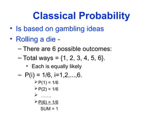
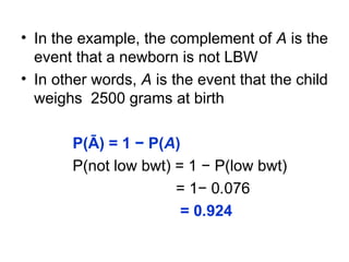
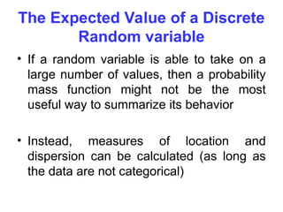
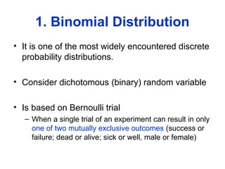
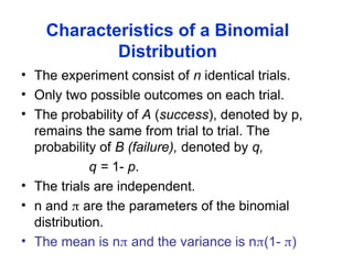
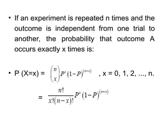
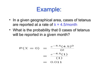
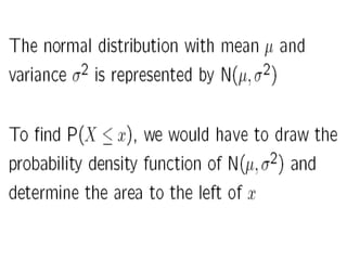
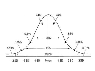
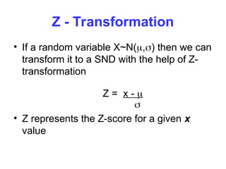
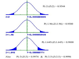
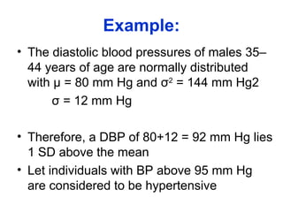
72. A binomial probability distribution occurs when
the following requirements are met.
1. The procedure has a fixed number of trials.
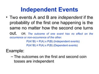
2. The trials must be independent.
3. Each trial must have all outcomes that fall
into two categories.
4. The probabilities must remain constant for
each trial [P(success) = p].

73. Characteristics of a Binomial
Distribution
• The experiment consist of n identical trials.
• Only two possible outcomes on each trial.
• The probability of A (success), denoted by p,
remains the same from trial to trial. The
probability of B (failure), denoted by q,
q = 1- p.
• The trials are independent.
• n and  are the parameters of the binomial
distribution.
• The mean is n and the variance is n(1- )

74. • Suppose an event can have only binary
outcomes A and B.
• Let the probability of A is  and that of B is
1 - .
• The probability  stays the same each
time the event occurs.

75. • If an experiment is repeated n times and the
outcome is independent from one trial to
another, the probability that outcome A
occurs exactly x times is:
• P (X=x) = , x = 0, 1, 2, ..., n.
=

76. • n denotes the number of fixed trials
• x denotes the number of successes in
the n trials
• p denotes the probability of success
• q denotes the probability of failure (1- p)
=
• Represents the number of ways of selecting x objects out of n
where the order of selection does not matter.
• where n!=n(n-1)(n-2)…(1) , and 0!=1

77. Example:
• Suppose we know that 40% of a certain
population are cigarette smokers. If we take
a random sample of 10 people from this
population, what is the probability that we
will have exactly 4 smokers in our sample?

78. • If the probability that any individual in the
population is a smoker to be P=.40, then the
probability that x=4 smokers out of n=10
subjects selected is:
P(X=4) =10C4(0.4)4
(1-0.4)10-4
= 10C4(0.4)4
(0.6)6
= 210(.0256)(.04666)
= 0.25
• The probability of obtaining exactly 4 smokers in
the sample is about 0.25.

79. • We can compute the probability of observing zero
smokers out of 10 subjects selected at random,
exactly 1 smoker, and so on, and display the
results in a table, as given, below.
• The third column, P(X ≤ x), gives the cumulative
probability. E.g. the probability of selecting 3 or
fewer smokers into the sample of 10 subjects is
P(X ≤ 3) =.3823, or about 38%.

81. The probability in the above table can
be converted into the following graph
0
0.05
0.1
0.15
0.2
0.25
0.3
0 1 2 3 4 5 6 7 8 9 10
No. of Smokers
Probability

82. Exercise
Each child born to a particular set of parents
has a probability of 0.25 of having blood type
O. If these parents have 5 children.
What is the probability that
a. Exactly two of them have blood type O
b. At most 2 have blood type O
c. At least 4 have blood type O
d. 2 do not have blood type O.

83. Solution for ‘a’
a.)
2637
.
0
)
75
.
0
(
)
25
.
0
(
2
5
=
2)
P(x 2
-
5
2









84. The Mean and Variance of a
Binomial Distribution
• Once n and P are specified, we can compute the
proportion of success,
P = x/n
• and the mean and variance of the distribution are
given by :
E(X) = μ = np, σ2
= npq, σ = √npq

85. Example:
• 70% of a certain population has been immunized
for polio. If a sample of size 50 is taken, what is
the “expected total number”, in the sample who
have been immunized?
µ = np = 50(.70) = 35
• This tells us that “on the average” we expect to
see 35 immunized subjects in a sample of 50
from this population.

86. • If repeated samples of size 10 are selected
from the population of infants born, the mean
number of children per sample who survive
to age 70 would be
µ = np = (10)(0.72) = 7.2
• The variance would be npq = (10)(0.72)
(0.28) = 2.02 and the SD would be
√2.02 = 1.42

87. 2. The Poisson Distribution
• Is a discrete probability distribution used to
model the number of occurrences of an
event that takes place infrequently in time
or space
• Applicable for counts of events over a given
interval of time, for example:
– number of patients arriving at an emergency
department in a day
– number of new cases of HIV diagnosed at a
clinic in a month

88. • In such cases, we take a sample of days
and observe the number of patients arriving
at the emergency department on each day,
• or a sample of months and observe the
number of new cases of HIV diagnosed at
the clinic.
• We are observing a count or number of
events, rather than a yes/no or success/
failure outcome for each subject or trial, as
in the binomial.

89. • In theory, a random variable X is a count
that can assume any integer value
greater than or equal to 0

90. • Suppose events happen randomly and
independently in time at a constant rate. If
events happen with rate  events per unit
time, the probability of x events happening
in unit time is:
P(x) =
e
x!
x
 


91. • where x = 0, 1, 2, . . .∞
• x is a potential outcome of X
• The constant λ (lambda) represents the
rate at which the event occurs, or the
expected number of events per unit time
• e = 2.71828
• It depends up on just one parameter, which
is the µ number of occurrences (λ).

92. • Three assumptions must be met for a
Poisson distribution to apply:
1. The probability that a single event occurs
within a given small subinterval is
proportional to the length of the subinterval
P(event) ≈ λΔt for constant λ
2. The rate at which the event occurs is
constant over the entire interval t
3. Events occurring in consecutive
subintervals are independent of each other

93. Example
• The daily number of new registrations of
cancer is 2.2 on average.
What is the probability of
a) Getting no new cases
b) Getting 1 case
c) Getting 2 cases
d) Getting 3 cases
e) Getting 4 cases

94. Solutions
a)
b) P(X=1) = 0.244
c) P(X=2) = 0.268
d) P(X=3) = 0.197
e) P(X=4) = 0.108
111
.
0
!
0
)
2
.
2
(
)
0
(
2
.
2
0




e
X
P

95. 0 1 2 3 4 5 6 7
0.3
0.2
0.1
0.0
Probability
Poisson distribution with mean 2.2

96. Example:
• In a given geographical area, cases of tetanus
are reported at a rate of λ = 4.5/month
• What is the probability that 0 cases of tetanus
will be reported in a given month?

97. • What is the probability that 1 case of
tetanus will be reported?

98. Characteristics
• The Poisson distribution is very asymmetric
when its mean is small
• With large means it becomes nearly
symmetric
• It has no theoretical maximum value, but the
probabilities tail off towards zero very quickly
 is the parameter of the Poisson distribution
• The mean is  and the variance is also .

99. B. Continuous Probability
Distributions
• A continuous random variable X can take on any
value in a specified interval or range
• With a large number of class intervals, the
frequency polygon begins to resemble a smooth
curve.
• The probability distribution of X is represented
by a smooth curve called a probability density
function

100. • The area under the smooth curve is equal to 1
• The area under the curve between any two points
x1 and x2 is the probability that X takes a value
between x1 and x2
Distribution of serum
triglyceride

101. • Instead of assigning probabilities to
specific outcomes of the random variable
X, probabilities are assigned to ranges of
values
• The probability associated with any one
particular value is equal to 0
• Therefore, P(X=x) = 0
• Also, P(X ≥ x) = P(X > x)

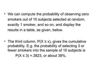
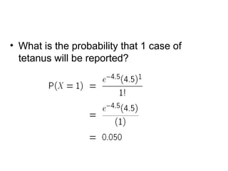
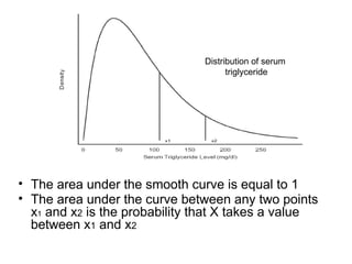
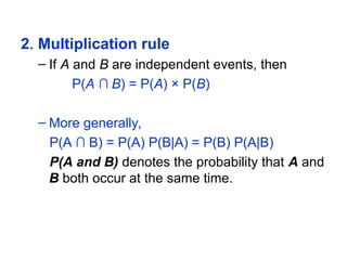
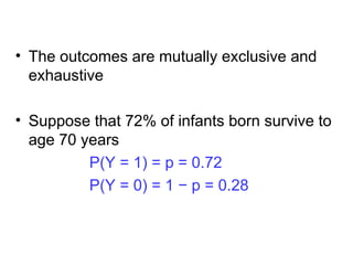
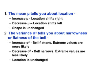
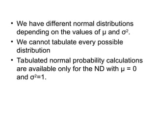
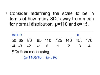
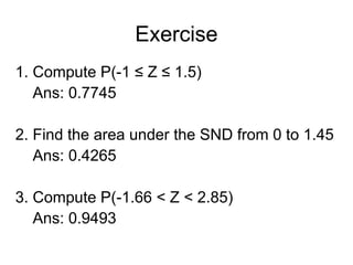
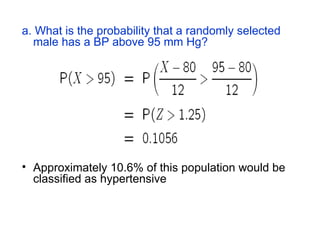
102. • We calculate:
Pr [ a < X < b], the probability of an
interval of values of X.
• For the above reason,
• is also without meaning.

103. The Normal distribution
• The ND is the most important probability
distribution in statistics
• Frequently called the “Gaussian distribution”
or bell-shape curve.
• Variables such as blood pressure, weight,
height, serum cholesterol level, and IQ
score — are approximately normally
distributed

104. A random variable is said to have a normal
distribution if it has a probability distribution
that is symmetric and bell-shaped

105. • The ND is vital to statistical work, most
estimation procedures and hypothesis tests
underlie ND
• The concept of “probability of X=x” in the
discrete probability distribution is replaced
by the “probability density function f(x)
• The ND is also an approximating distribution
to other distributions (e.g., binomial)

106. • A random variable X is said to follow ND, if
and only if, its probability density function
is:
, - < x < .
f(x) =
1
2
e
x-
2
 









1
2

107. π (pi) = 3.14159
e = 2.71828, x = Value of X
Range of possible values of X: -∞ to +∞
µ = Expected value of X (“the long run
average”)
σ2
= Variance of X.
µ and σ are the parameters of the normal
distribution — they completely define its
shape

109. 1. The mean µ tells you about location -
– Increase µ - Location shifts right
– Decrease µ – Location shifts left
– Shape is unchanged
2. The variance σ2
tells you about narrowness
or flatness of the bell -
– Increase σ2
- Bell flattens. Extreme values are
more likely
– Decrease σ2
- Bell narrows. Extreme values are
less likely
– Location is unchanged

111. Properties of the Normal Distribution
1. It is symmetrical about its mean, .
2. The mean, the median and mode are
almost equal. It is unimodal.
3. The total area under the curve about the x-
axis is 1 square unit.
4. The curve never touches the x-axis.
5. As the value of  increases, the curve
becomes more and more flat and vice
versa.

112. 6. Perpendiculars of:
± SD contain about 68%;
±2 SD contain about 95%;
±3 SD contain about 99.7%
of the area under the curve.
Next slide
7. The distribution is completely determined
by the parameters  and .

114. • We have different normal distributions
depending on the values of μ and σ2
.
• We cannot tabulate every possible
distribution
• Tabulated normal probability calculations
are available only for the ND with µ = 0
and σ2
=1.

115. Standard Normal Distribution
 It is a normal distribution that has a mean
equal to 0 and a SD equal to 1, and is
denoted by N(0, 1).
 The main idea is to standardize all the
data that is given by using Z-scores.
 These Z-scores can then be used to find
the area (and thus the probability) under
the normal curve.

116. The standard normal distribution has
mean 0 and variance 1
• Approximately 68% of the area under the standard
normal curve lies between ±1, about 95% between ±2,
and about 99% between ±2.5

117. Z - Transformation
• If a random variable X~N(,) then we can
transform it to a SND with the help of Z-
transformation
Z = x - 

• Z represents the Z-score for a given x
value

118. • Consider redefining the scale to be in
terms of how many SDs away from mean
for normal distribution, μ=110 and σ=15.
Value x
50 65 80 95 110 125 140 155 170
-4 -3 -2 -1 0 1 2 3 4
SDs from mean using
(x-110)/15 = (x-μ)/σ

119. • This process is known as standardization
and gives the position on a normal curve
with μ=0 and σ=1, i.e., the SND, Z.
• A Z-score is the number of standard
deviations that a given x value is above or
below the mean.

120. Finding normal curve areas
1. The table gives areas between -∞ and the value
of zo.
2. Find the z value in tenths in the column at left
margin and locate its row. Find the hundredths
place in the appropriate column.
3. Read the value of the area (P) from the body of
the table where the row and column intersect.
Values of P are in the form of a decimal point and
four places.

121. Some Useful Tips

122. a) What is the probability that z < -1.96?
(1) Sketch a normal curve
(2) Draw a perpendicular line for z = -1.9
(3) Find the area in the table
(4) The answer is the area to the left of the line P(z
< -1.96) = 0.0250

123. b) What is the probability that -1.96 < z <
1.96?
The area between the values P(-1.96 < z <
1.96) = .9750 - .0250 = .9500

124. c) What is the probability that z > 1.96?
• The answer is the area to the right of the line; found by
subtracting table value from 1.0000; P(z > 1.96) =1.0000
- .9750 = .0250

126. Exercise
1. Compute P(-1 ≤ Z ≤ 1.5)
Ans: 0.7745
2. Find the area under the SND from 0 to 1.45
Ans: 0.4265
3. Compute P(-1.66 < Z < 2.85)
Ans: 0.9493

127. Applications of the Normal
Distribution
• The ND is used as a model to study many
different variables.
• The ND can be used to answer probability
questions about continuous random variables.
• Following the model of the ND, a given value of
x must be converted to a z score before it can
be looked up in the z table.

128. Example:
• The diastolic blood pressures of males 35–
44 years of age are normally distributed
with µ = 80 mm Hg and σ2
= 144 mm Hg2
σ = 12 mm Hg
• Therefore, a DBP of 80+12 = 92 mm Hg lies
1 SD above the mean
• Let individuals with BP above 95 mm Hg
are considered to be hypertensive

129. a. What is the probability that a randomly selected
male has a BP above 95 mm Hg?
• Approximately 10.6% of this population would be
classified as hypertensive

130. b. What is the probability that a randomly
selected male has a DBP above 110 mm
Hg?
Z = 110 – 80 = 2.50
12
P (Z > 2.50) = 0.0062
• Approximately 0.6% of the population has a
DBP above 110 mm Hg

131. c. What is the probability that a randomly
selected male has a DBP below 60 mm Hg?
Z = 60 – 80 = -1.67
12
P (Z < -1.67) = 0.0475
• Approximately 4.8% of the population has a
DBP below 60 mm Hg

132. d. What value of DBP cuts off the upper 5% of this
population?
• Looking at the table, the value Z = 1.645 cuts off
an area of 0.05 in the upper tail
• We want the value of X that corresponds to Z =
1.645
Z = X – μ
σ
1.645 = X – μ, X = 99.7
σ
• Approximately 5% of the men in this population
have a DBP greater than 99.7 mm Hg

133. Other Distributions
1. Student t-distribution
2. F- Distribution
3. 2
-Distribution