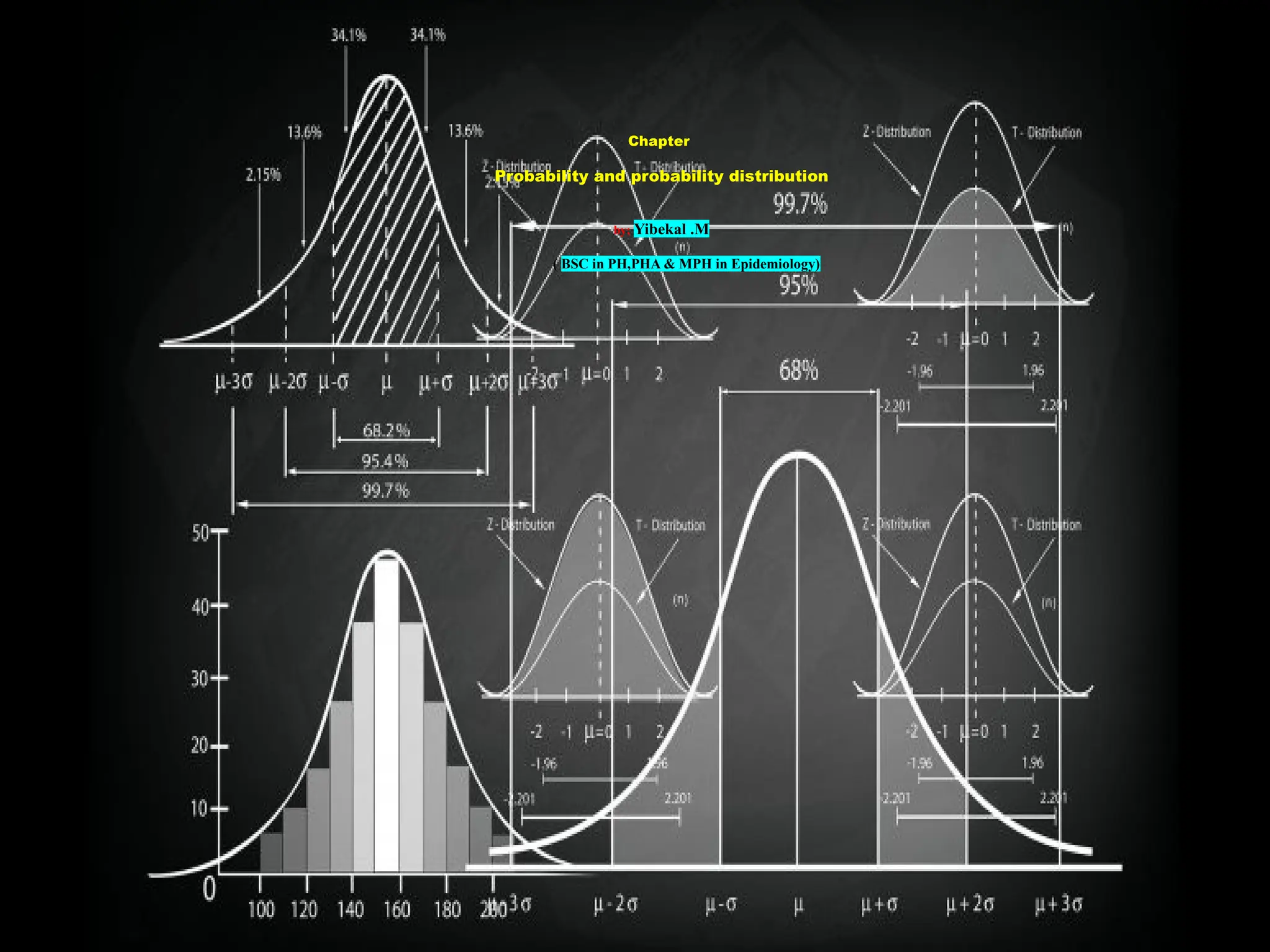
04/04/2025 Yibekal.M(MPH) inEpidemiology 3
At the end of this chapter, students are expected to understand the following
§ Probability
§ The difference between probability and probability
distribution
§ Conditional probability
§ Distribution for categorical variable
§ Distribution for continuous variable
§ Different distribution tables
a b
4.
04/04/2025 Yibekal.M(MPH) inEpidemiology 4
Chance
• When a meteorologist states that the chance of rain is 50%,
the meteorologist is saying that it is equally likely to rain or
not to rain. If the chance of rain rises to 80%, it is more likely
to rain. If the chance drops to 20%, then it may rain, but it
probably will not rain.
• These examples suggest the chance of an
occurrence of some event of a random variable.
5.
04/04/2025 Yibekal.M(MPH) inEpidemiology 5
Probability and Probability
Distributions
Probabilities and probability distributions
are nothing more than extensions of the
ideas of relative frequency and histograms,
respectively.
6.
04/04/2025 Yibekal.M(MPH) inEpidemiology 6
Why Probability in Medicine?
• Because medicine is an inexact science,
physicians seldom predict an outcome with
absolute certainty.
• E.g., to formulate a diagnosis, a physician must
rely on available diagnostic information about a
patient
– History and physical examination
– Laboratory investigation, X-ray findings, ECG, etc
7.
04/04/2025 Yibekal.M(MPH) inEpidemiology 7
Cont…
• An understanding of probability is fundamental
for quantifying the uncertainty that is inherent in
the decision-making process.
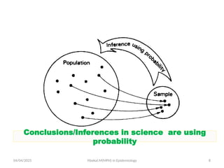
• Probability theory also allows us to draw
conclusions about a population based on
known information about a sample which drown
from that population.
04/04/2025 Yibekal.M(MPH) inEpidemiology 9
Terminology
Random experiment/ random variable: is one in
which the out comes occur at random or cannot
be predicted with certainty.
e.g. A single coin tossing experiment is a random as the
occurrence of Head(H) and Tail(T)
Trial: A physical action , the result of which cannot
be predetermined
.
10.
04/04/2025 Yibekal.M(MPH) inEpidemiology 10
Terminology…
Sample Space: The set of all possible outcomes of an
experiment .
In die throwing, S={1,2,3,4,5,6}
Events: Collections of basic outcomes from the sample space.
We say that an event occurs if any one of the basic outcomes in
the event occurs.
Any subset of sample space.
- Event of getting even number A={2,4,6}
Success/ favorable case: Outcome that entail the happening of
a desired event.
11.
04/04/2025 Yibekal.M(MPH) inEpidemiology 11
Equally likely events:
If in a random experiment all out comes have
equal chance of occurrence.
- In tossing coin both H and T have equal chance to occur
Mutually Exclusive Events (Disjoint Events)
If the occurrence of one event prevent the
occurrence of the other.
- In tossing coin the occurrence of Head prevent the
occurrence of Tail.
12.
04/04/2025 Yibekal.M(MPH) inEpidemiology 12
Cont…
Independent events(mutual independence)
The occurrence or non-occurrence of one event
doesn’t affect the occurrence or non-occurrence
of the other event in repeated trials, conduction
of a random experiment.
While tossing of two coin simultaneously, the occurrence of
head in one coin does not affect the occurrence of tail on the
other.
13.
04/04/2025 Yibekal.M(MPH) inEpidemiology 13
Two Categories of Probability
• Objective and Subjective Probabilities.
• Objective probability
1) Classical probability and
2) Relative frequency probability.
14.
04/04/2025 Yibekal.M(MPH) inEpidemiology 14
Types of probability
Classical Method
If there are n equally likely possibilities, of
which one must occur and m are regarded as
favorable, or as a “success,” then the probability
of a “success” is m/n.
P(A) = m/n
What is the probability of rolling a 6 with a well-balanced
die? Ans.
In this case, m=1 and n=6, so that the probability is 1/6
= 0.167
15.
04/04/2025 Yibekal.M(MPH) inEpidemiology 15
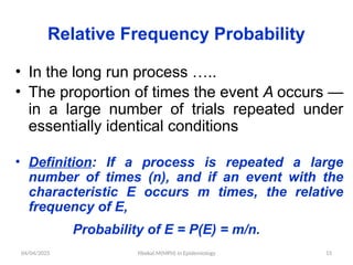
Relative Frequency Probability
• In the long run process …..
• The proportion of times the event A occurs —
in a large number of trials repeated under
essentially identical conditions
• Definition: If a process is repeated a large
number of times (n), and if an event with the
characteristic E occurs m times, the relative
frequency of E,
Probability of E = P(E) = m/n.
16.
04/04/2025 Yibekal.M(MPH) inEpidemiology 16
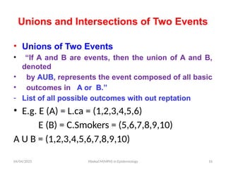
Unions and Intersections of Two Events
• Unions of Two Events
• “If A and B are events, then the union of A and B,
denoted
• by AUB, represents the event composed of all basic
• outcomes in A or B.”
- List of all possible outcomes with out reptation
• E.g. E (A) = L.ca = (1,2,3,4,5,6)
E (B) = C.Smokers = (5,6,7,8,9,10)
A U B = (1,2,3,4,5,6,7,8,9,10)
17.
04/04/2025 Yibekal.M(MPH) inEpidemiology 17
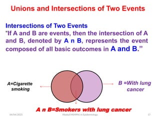
Intersections of Two Events
“If A and B are events, then the intersection of A
and B, denoted by A n B, represents the event
composed of all basic outcomes in A and B.”
Unions and Intersections of Two Events
B =With lung
cancer
A=Cigarette
smoking
A n B=Smokers with lung cancer
18.
04/04/2025 Yibekal.M(MPH) inEpidemiology 18
Properties of Probability
1. The numerical value of a probability always
lies between 0 and 1, inclusive.
0 P(E) 1
A value 0 means the event can not occur
A value 1 means the event definitely will occur
A value of 0.5 means that the probability that
the event will occur is the same as the
probability that it will not occur.
19.
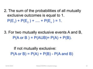
04/04/2025 Yibekal.M(MPH) inEpidemiology 19
2. The sum of the probabilities of all mutually
exclusive outcomes is equal to 1.
P(E1
) + P(E2
) + .... + P(En
) = 1.
3. For two mutually exclusive events A and B,
P(A or B ) = P(AUB)= P(A) + P(B).
If not mutually exclusive:
P(A or B) = P(A) + P(B) - P(A and B)
20.
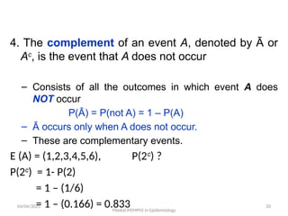
04/04/2025 20
4. Thecomplement of an event A, denoted by Ā or
Ac
, is the event that A does not occur
– Consists of all the outcomes in which event A does
NOT occur
P(Ā) = P(not A) = 1 – P(A)
– Ā occurs only when A does not occur.
– These are complementary events.
E (A) = (1,2,3,4,5,6), P(2c
) ?
P(2c
) = 1- P(2)
= 1 – (1/6)
= 1 – (0.166) = 0.833
Yibekal.M(MPH) in Epidemiology
21.
04/04/2025 Yibekal.M(MPH) inEpidemiology 21
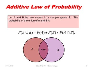
Additive Law of Probability
Let A and B be two events in a sample space S. The
probability of the union of A and B is
( ) ( ) ( ) ( ).
P A B P A P B P A B
B
A A n B
22.
04/04/2025 Yibekal.M(MPH) inEpidemiology 22
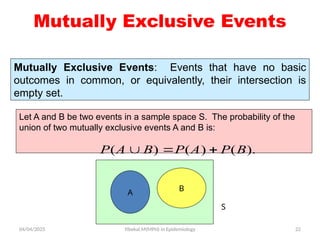
Mutually Exclusive Events
Mutually Exclusive Events: Events that have no basic
outcomes in common, or equivalently, their intersection is
empty set.
S
B
A
Let A and B be two events in a sample space S. The probability of the
union of two mutually exclusive events A and B is:
( ) ( ) ( ).
P A B P A P B
23.
04/04/2025 Yibekal.M(MPH) inEpidemiology 23
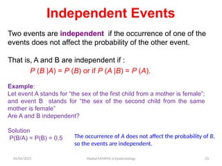
Two events are independent if the occurrence of one of the
events does not affect the probability of the other event.
That is, A and B are independent if :
P (B |A) = P (B) or if P (A |B) = P (A).
Independent Events
Example:
Let event A stands for “the sex of the first child from a mother is female”;
and event B stands for “the sex of the second child from the same
mother is female”
Are A and B independent?
Solution
P(B/A) = P(B) = 0.5 The occurrence of A does not affect the probability of B,
so the events are independent.
24.
04/04/2025 Yibekal.M(MPH) inEpidemiology 24
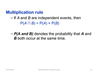
Multiplication rule
– If A and B are independent events, then
P(A ∩ B) = P(A) × P(B)
– P(A and B) denotes the probability that A and
B both occur at the same time.
25.
04/04/2025 Yibekal.M(MPH) inEpidemiology 25
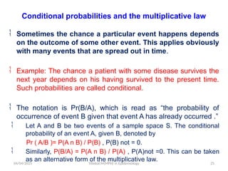
Conditional probabilities and the multiplicative law
Sometimes the chance a particular event happens depends
on the outcome of some other event. This applies obviously
with many events that are spread out in time.
Example: The chance a patient with some disease survives the
next year depends on his having survived to the present time.
Such probabilities are called conditional.
The notation is Pr(B/A), which is read as “the probability of
occurrence of event B given that event A has already occurred .”
Let A and B be two events of a sample space S. The conditional
probability of an event A, given B, denoted by
Pr ( A/B )= P(A n B) / P(B) , P(B) not = 0.
Similarly, P(B/A) = P(A n B) / P(A) , P(A)not =0. This can be taken
as an alternative form of the multiplicative law.
26.
04/04/2025 Yibekal.M(MPH) inEpidemiology 26
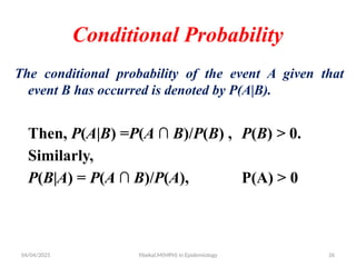
Conditional Probability
The conditional probability of the event A given that
event B has occurred is denoted by P(A|B).
Then, P(A|B) =P(A ∩ B)/P(B) , P(B) > 0.
Similarly,
P(B|A) = P(A ∩ B)/P(A), P(A) > 0
27.
04/04/2025 Yibekal.M(MPH) inEpidemiology 27
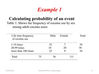
Example 1
Calculating probability of an event
Table 1: Shows the frequency of cocaine use by sex
among adult cocaine users
_______________________________________________________________________________________________
Life time frequency Male Female Total
of cocaine use
_______________________________________________________________________________________________
1-19 times 32 7 39
20-99 times 18 20 38
more than 100 times 25 9 34
--------------------------------------------------------------------------------------------
Total 75 36 111
---------------------------------------------------------------------------------------------
28.
04/04/2025 Yibekal.M(MPH) inEpidemiology 28
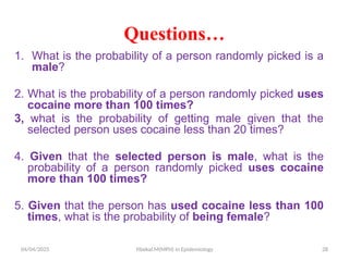
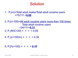
Questions…
1. What is the probability of a person randomly picked is a
male?
2. What is the probability of a person randomly picked uses
cocaine more than 100 times?
3, what is the probability of getting male given that the
selected person uses cocaine less than 20 times?
4. Given that the selected person is male, what is the
probability of a person randomly picked uses cocaine
more than 100 times?
5. Given that the person has used cocaine less than 100
times, what is the probability of being female?
04/04/2025 Yibekal.M(MPH) inEpidemiology 31
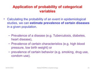
Application of probability of categorical
variables
• Calculating the probability of an event in epidemiological
studies, we can estimate prevalence of certain diseases
in a given population.
– Prevalence of a disease (e.g. Tuberculosis, diabetes,
heart disease),
– Prevalence of certain characteristics (e.g. high blood
pressure, low birth weight) or
– prevalence of certain behavior (e.g. smoking, drug use,
condom use).
31.
04/04/2025 Yibekal.M(MPH) inEpidemiology 32
Probability Distributions
• A probability distribution is a device used to
describe the behavior that a random variable may
have by applying the theory of probability.
• It is the way data are distributed, in order to draw
conclusions about a set of data
• Random Variable = Any quantity or characteristic
that is able to assume a number of different values
such that any particular outcome is determined by
chance
32.
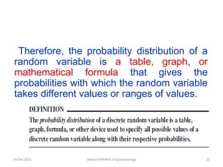
04/04/2025 Yibekal.M(MPH) inEpidemiology 33
Therefore, the probability distribution of a
random variable is a table, graph, or
mathematical formula that gives the
probabilities with which the random variable
takes different values or ranges of values.
33.
04/04/2025 Yibekal.M(MPH) inEpidemiology 34
A. Discrete Probability Distributions
• For a discrete random variable, the probability
distribution specifies each of the possible
outcomes of the random variable along with the
probability that each will occur
• Examples can be:
– Frequency distribution
– Relative frequency distribution
– Cumulative frequency
34.
04/04/2025 Yibekal.M(MPH) inEpidemiology 35
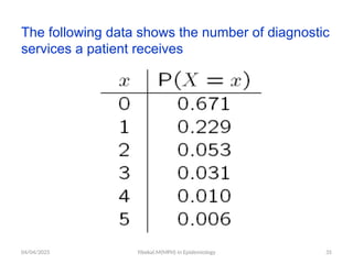
The following data shows the number of diagnostic
services a patient receives
35.
04/04/2025 Yibekal.M(MPH) inEpidemiology 36
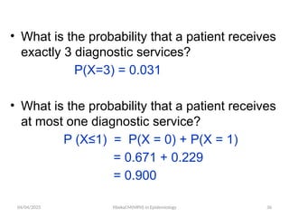
• What is the probability that a patient receives
exactly 3 diagnostic services?
P(X=3) = 0.031
• What is the probability that a patient receives
at most one diagnostic service?
P (X≤1) = P(X = 0) + P(X = 1)
= 0.671 + 0.229
= 0.900
36.
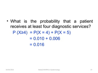
04/04/2025 Yibekal.M(MPH) inEpidemiology 37
• What is the probability that a patient
receives at least four diagnostic services?
P (X≥4) = P(X = 4) + P(X = 5)
= 0.010 + 0.006
= 0.016
37.
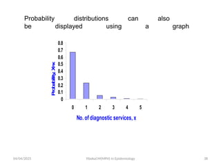
04/04/2025 Yibekal.M(MPH) inEpidemiology 38
Probability distributions can also
be displayed using a graph
0
0.1
0.2
0.3
0.4
0.5
0.6
0.7
0.8
0 1 2 3 4 5
No. of diagnostic services, x
P
ro
b
a
b
ility
,
X
=
x
38.
04/04/2025 Yibekal.M(MPH) inEpidemiology 39
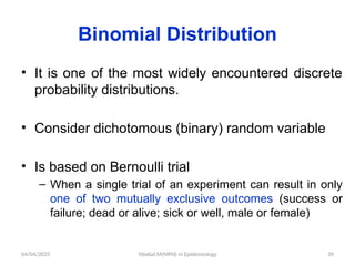
Binomial Distribution
• It is one of the most widely encountered discrete
probability distributions.
• Consider dichotomous (binary) random variable
• Is based on Bernoulli trial
– When a single trial of an experiment can result in only
one of two mutually exclusive outcomes (success or
failure; dead or alive; sick or well, male or female)
39.
04/04/2025 Yibekal.M(MPH) inEpidemiology 40
A binomial probability distribution occurs when
the following requirements are met.
1. The procedure has a fixed number of trials.
2. The trials must be independent.
3. Each trial must have all outcomes that fall into
two categories.
4. The probabilities must remain constant for each
trial [P(success) = p].
40.
04/04/2025 Yibekal.M(MPH) inEpidemiology 49
B. Probability distribution of continuous variables
• Under different circumstances, the outcome of a random
variable may not be limited to categories or counts.
– E.g. Suppose, X represents the continuous variable
‘Height’; rarely is an individual exactly equal to 170cm tall.
– X can assume an infinite number of intermediate values
170.1, 170.2, 170.3 etc.
• Because a continuous random variable X can take on an
infinite number of values, the probability associated with
any particular one value is almost equal to zero.
04/04/2025 Yibekal.M(MPH) inEpidemiology 51
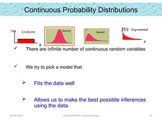
Continuous Probability Distributions
There are infinite number of continuous random variables
We try to pick a model that
Fits the data well
Allows us to make the best possible inferences
using the data.
f (x)
x
Uniform Normal Skewed
43.
04/04/2025 Yibekal.M(MPH) inEpidemiology 52
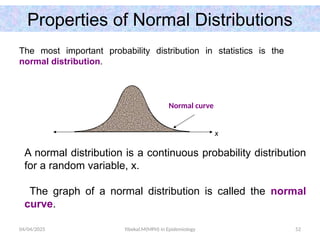
Properties of Normal Distributions
The most important probability distribution in statistics is the
normal distribution.
A normal distribution is a continuous probability distribution
for a random variable, x.
The graph of a normal distribution is called the normal
curve.
Normal curve
x
44.
04/04/2025 Yibekal.M(MPH) inEpidemiology 53
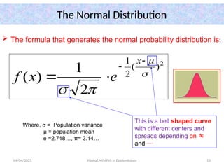
The Normal Distribution
The formula that generates the normal probability distribution is:
Where, s = Population variance
µ = population mean
e =2.718…, π= 3.14…
2
)
(
2
1
2
1
)
(
x
e
x
f
This is a bell shaped curve
with different centers and
spreads depending on
and
45.
04/04/2025 Yibekal.M(MPH) inEpidemiology 54
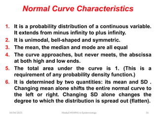
Normal Curve Characteristics
1. It is a probability distribution of a continuous variable.
It extends from minus infinity to plus infinity.
2. It is unimodal, bell-shaped and symmetric.
3. The mean, the median and mode are all equal
4. The curve approaches, but never meets, the abscissa
at both high and low ends.
5. The total area under the curve is 1. (This is a
requirement of any probability density function.)
6. It is determined by two quantities: its mean and SD .
Changing mean alone shifts the entire normal curve to
the left or right. Changing SD alone changes the
degree to which the distribution is spread out (flatten).
04/04/2025 Yibekal.M(MPH) inEpidemiology 56
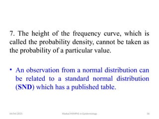
7. The height of the frequency curve, which is
called the probability density, cannot be taken as
the probability of a particular value.
• An observation from a normal distribution can
be related to a standard normal distribution
(SND) which has a published table.
48.
04/04/2025 Yibekal.M(MPH) inEpidemiology 57
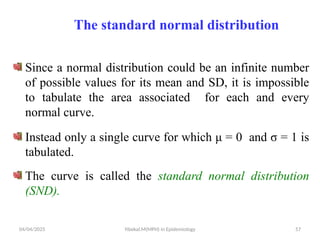
The standard normal distribution
Since a normal distribution could be an infinite number
of possible values for its mean and SD, it is impossible
to tabulate the area associated for each and every
normal curve.
Instead only a single curve for which μ = 0 and σ = 1 is
tabulated.
The curve is called the standard normal distribution
(SND).
49.
04/04/2025 Yibekal.M(MPH) inEpidemiology 58
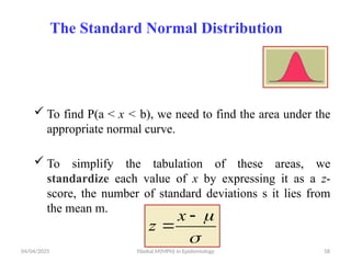
The Standard Normal Distribution
To find P(a < x < b), we need to find the area under the
appropriate normal curve.
To simplify the tabulation of these areas, we
standardize each value of x by expressing it as a z-
score, the number of standard deviations s it lies from
the mean m.
x
z
50.
04/04/2025 Yibekal.M(MPH) inEpidemiology 59
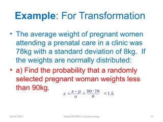
• The average weight of pregnant women
attending a prenatal care in a clinic was
78kg with a standard deviation of 8kg. If
the weights are normally distributed:
• a) Find the probability that a randomly
selected pregnant woman weights less
than 90kg.
Example: For Transformation
-
90-78
=
8
x μ
z
σ
= 1.5
51.
04/04/2025 Yibekal.M(MPH) inEpidemiology 60
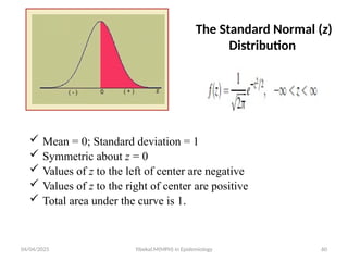
The Standard Normal (z)
Distribution
Mean = 0; Standard deviation = 1
Symmetric about z = 0
Values of z to the left of center are negative
Values of z to the right of center are positive
Total area under the curve is 1.
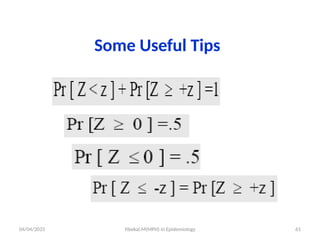
04/04/2025 Yibekal.M(MPH) inEpidemiology 62
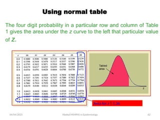
Using normal table
The four digit probability in a particular row and column of Table
1 gives the area under the z curve to the left that particular value
of z.
Area for z 1.36
54.
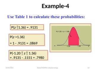
04/04/2025 Yibekal.M(MPH) inEpidemiology 63
P(z 1.36) = .9131
P(z >1.36)
= 1 - .9131 = .0869
P(-1.20 z 1.36)
= .9131 - .1151 = .7980
Example-4
Use Table 1 to calculate these probabilities:
55.
04/04/2025 Yibekal.M(MPH) inEpidemiology 65
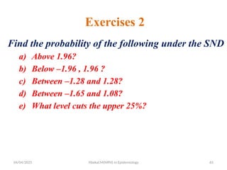
Exercises 2
Find the probability of the following under the SND
a) Above 1.96?
b) Below –1.96 , 1.96 ?
c) Between –1.28 and 1.28?
d) Between –1.65 and 1.08?
e) What level cuts the upper 25%?
56.
04/04/2025 Yibekal.M(MPH) inEpidemiology 66
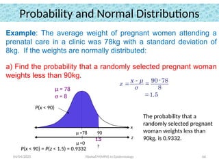
Example: The average weight of pregnant women attending a
prenatal care in a clinic was 78kg with a standard deviation of
8kg. If the weights are normally distributed:
a) Find the probability that a randomly selected pregnant woman
weights less than 90kg.
Probability and Normal Distributions
P(x < 90) = P(z < 1.5) = 0.9332
-
90-78
=
8
x μ
z
σ
= 1.5
The probability that a
randomly selected pregnant
woman weights less than
90kg. is 0.9332.
μ =0
z
?
1.5
90
μ =78
P(x < 90)
μ = 78
σ = 8
x
57.
04/04/2025 Yibekal.M(MPH) inEpidemiology 67
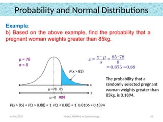
Example:
b) Based on the above example, find the probability that a
pregnant woman weights greater than 85kg.
Probability and Normal Distributions
P(x > 85) = P(z > 0.88) = 1 P(z < 0.88) = 1 0.8106 = 0.1894
85-78
= =
8
x - μ
z
σ
= 0.875 0.88
The probability that a
randomly selected pregnant
woman weights greater than
85kg. is 0.1894.
μ =0
z
?
0.88
85
μ =78
P(x > 85)
μ = 78
σ = 8
x
#34 The probability distribution of a discrete random variable is a table, graph, formula, or other device used to specify all possible values of a discrete random variable along with their respective probabilities. The relationship between the values and their associated probabilities is called a probability mass function.
#36 Many random variables are displayed in tables or figures in terms of a cumulative distribution function rather than a distribution of probabilities of individual values. The basic concept is to assign to each individual value the sum of probabilities of all values that are no larger than the value being considered. Thus, the cumulative distribution function of a random variable X is denoted by F(X) and, for a specific value x of X, is defined by P(X≤ x) and denoted by F(x).
#39 In a sample of n independent trials, each of which can have only two possible outcomes. denoted as “success” and “failure”.
#48 Note that, although p is a fraction, its sampling distribution is discrete and not continuous, since it may take only a limited number of values for any given sample size.
As the sample size n increases the binomial distribution becomes very close to a normal distribution, and this can be used to calculate confidence intervals and carry out hypothesis tests.
In fact the normal distribution can be used as a reasonable approximation to the binomial distribution if both np and n-np are 10 or more. This approximating normal distribution has the same mean and standard error as the binomial distribution.


![04/04/2025 Yibekal.M(MPH) in Epidemiology 40
A binomial probability distribution occurs when
the following requirements are met.
1. The procedure has a fixed number of trials.
2. The trials must be independent.
3. Each trial must have all outcomes that fall into
two categories.
4. The probabilities must remain constant for each
trial [P(success) = p].](https://image.slidesharecdn.com/chapter4all-copy-250404201714-fc12bd73/85/chapter_4_All-Copy-pptx-39-320.jpg)


![ch_5-8_probability155[1].ppt](https://cdn.slidesharecdn.com/ss_thumbnails/ch5-8probability1551-231116061842-b428d0bc-thumbnail.jpg?width=640&height=640&fit=bounds)


