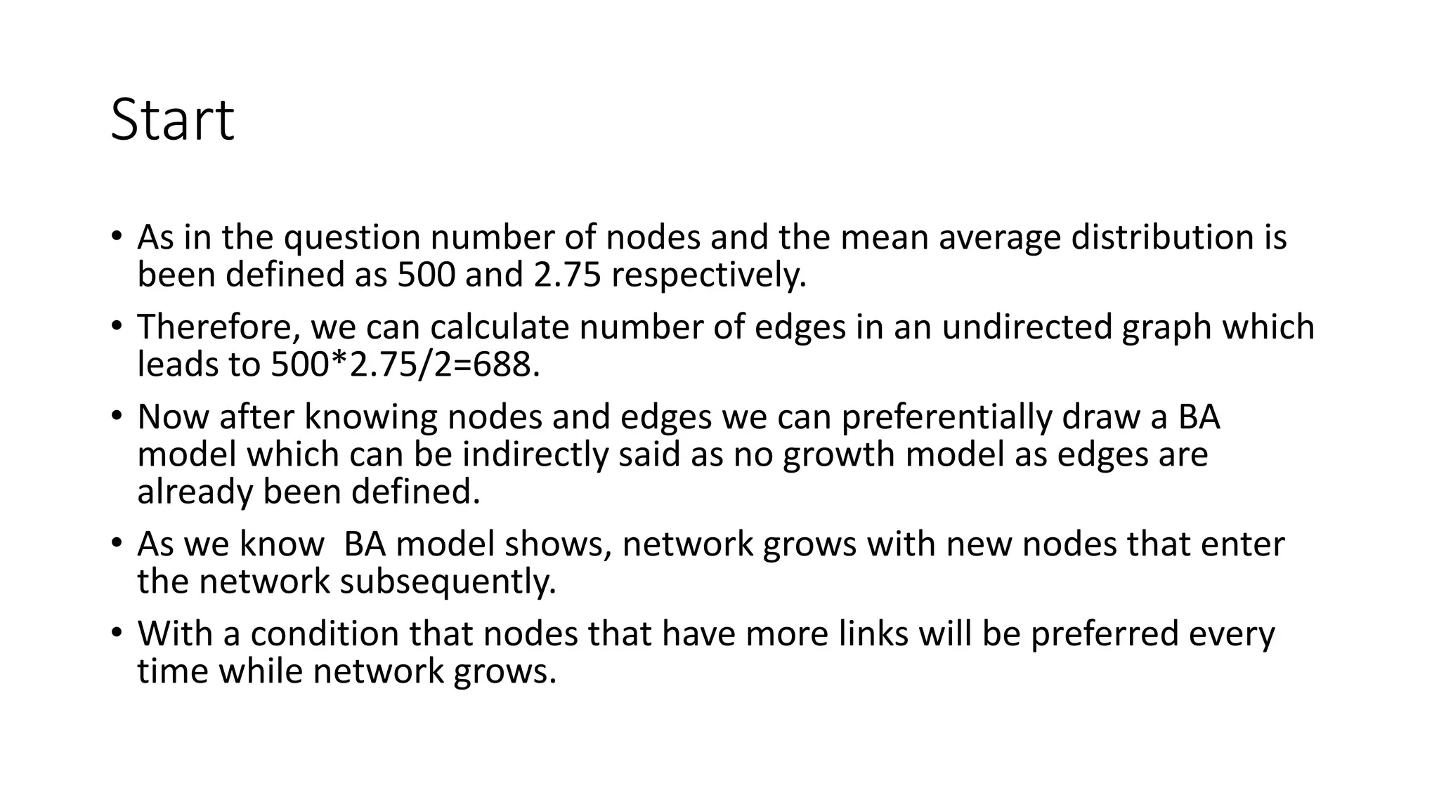
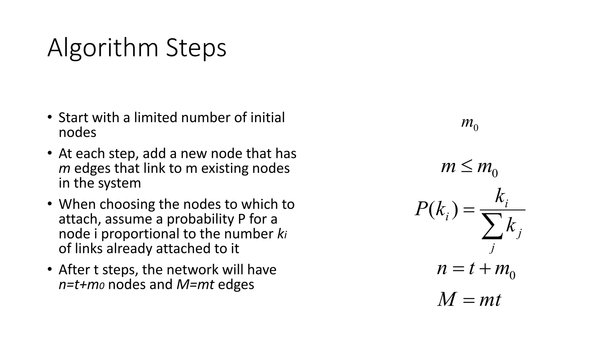
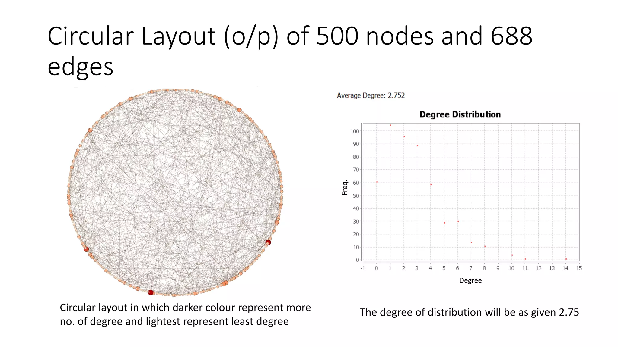
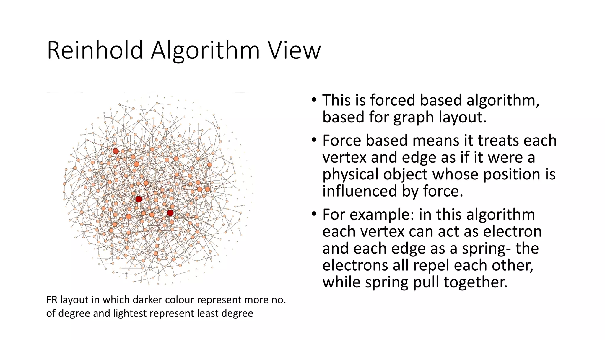
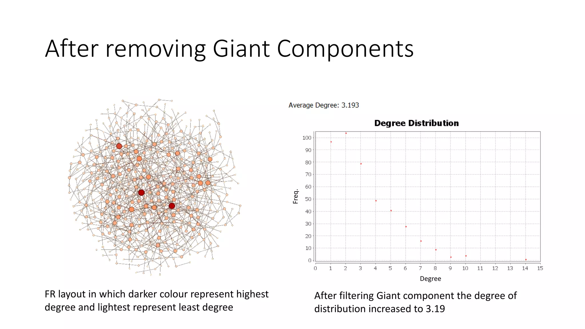
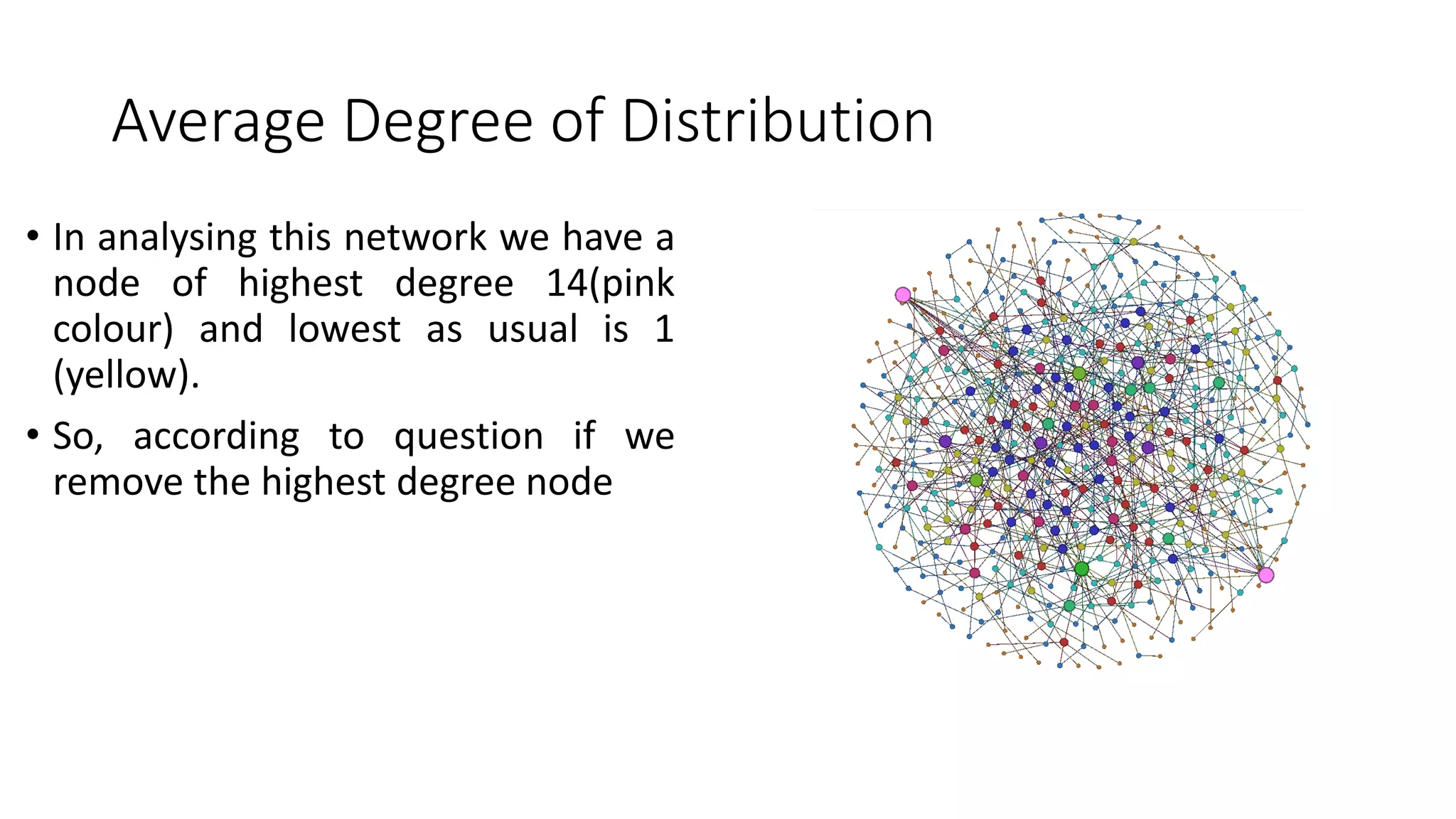
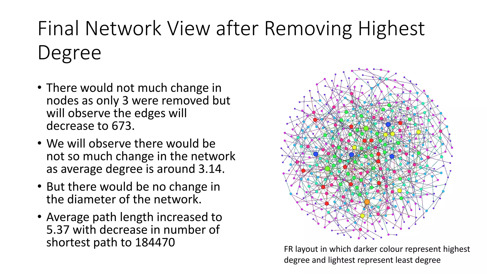
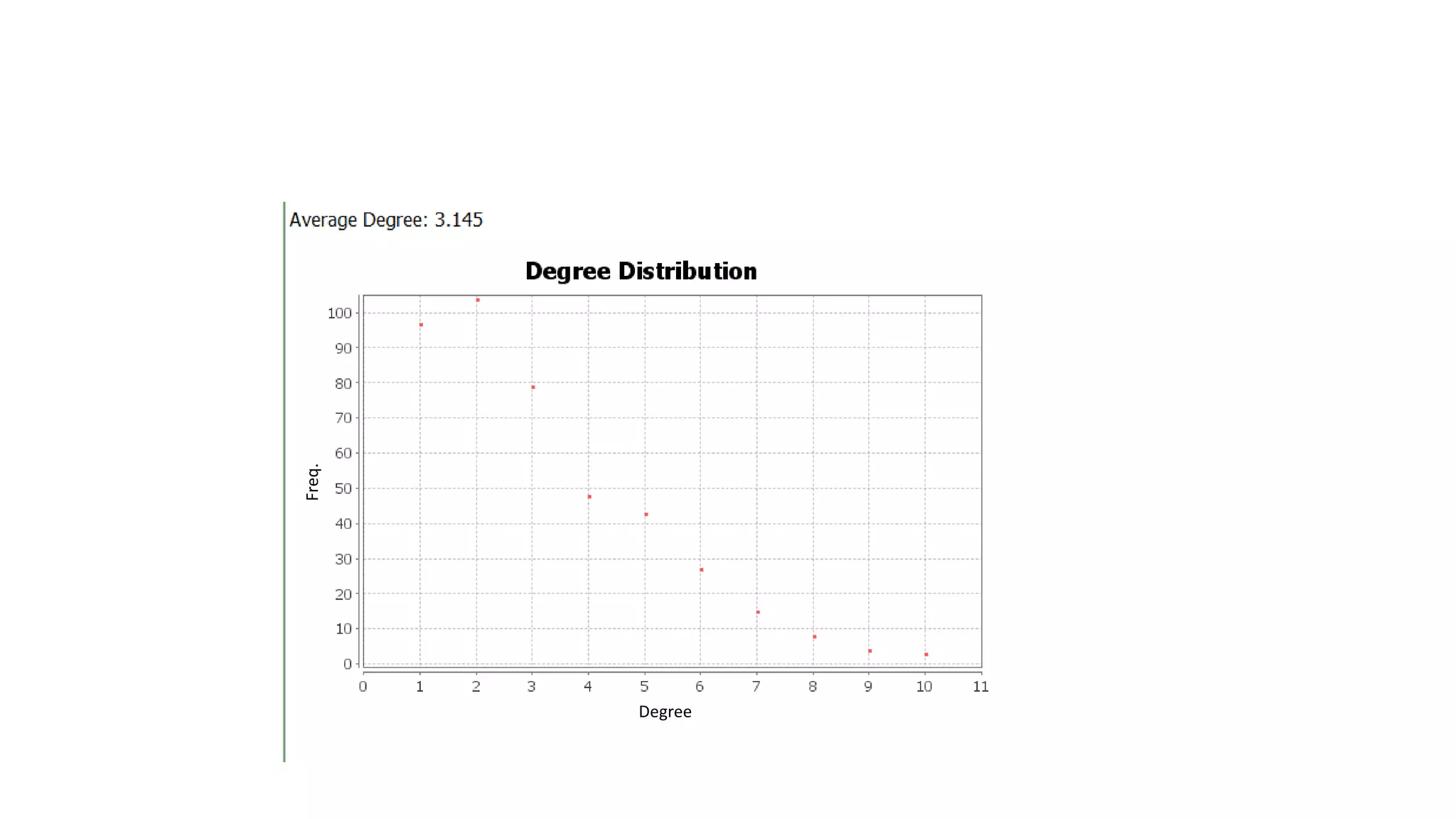
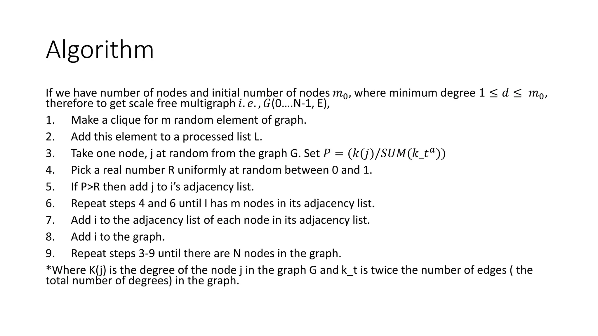
The document describes generating and analyzing a scale-free network using the Barabási-Albert (BA) preferential attachment model and Fruchterman-Reingold (FR) force-directed graph drawing algorithm. Key points: - The BA model is used to generate an undirected scale-free network with 500 nodes and approximately 688 edges based on the given mean degree of 2.75. - Degree distribution and circular layout are analyzed for the initial BA network. Giant components are then removed, increasing the average degree to 3.19. - The FR algorithm is applied to visualize the network, treating nodes as electrons and edges as springs. Darker colors represent higher-degree nodes.

1. Visualizing Scale Free Network
with the help of BA and FR
algorithm
By,
Harshit Srivastava
D03942013

2. Start
• As in the question number of nodes and the mean average distribution is
been defined as 500 and 2.75 respectively.
• Therefore, we can calculate number of edges in an undirected graph which
leads to 500*2.75/2=688.
• Now after knowing nodes and edges we can preferentially draw a BA
model which can be indirectly said as no growth model as edges are
already been defined.
• As we know BA model shows, network grows with new nodes that enter
the network subsequently.
• With a condition that nodes that have more links will be preferred every
time while network grows.

3. Algorithm Steps
• Start with a limited number of initial
nodes
• At each step, add a new node that has
m edges that link to m existing nodes
in the system
• When choosing the nodes to which to
attach, assume a probability P for a
node i proportional to the number ki
of links already attached to it
• After t steps, the network will have
n=t+m0 nodes and M=mt edges
0m
0mm 


j
j
i
i
k
k
kP )(
mtM
mtn

 0

4. Distribution Algorithm
• Then for finding distribution just,
• Initially find how many connection each node has.
• Initialize variable that will hold how many nodes have each degree.
• This variable will be used to create a list of possible degrees a node
can have
• Dismantle the degrees with no connectivity
• Find the last non zero element.
• Plot these variables in respect of connectivity.

5. Circular Layout (o/p) of 500 nodes and 688
edges
Degree
Freq.
Circular layout in which darker colour represent more
no. of degree and lightest represent least degree
The degree of distribution will be as given 2.75

6. Reinhold Algorithm View
• This is forced based algorithm,
based for graph layout.
• Force based means it treats each
vertex and edge as if it were a
physical object whose position is
influenced by force.
• For example: in this algorithm
each vertex can act as electron
and each edge as a spring- the
electrons all repel each other,
while spring pull together.
FR layout in which darker colour represent more no.
of degree and lightest represent least degree

7. Algorithm Steps
• Define the width and length of the layout which is to be used.
• Draw a graph G(V,E) randomly, and repeat it M times.
• Then calculate repulsive forces on each vertex/electron,
• Move the vertex will be having two information: position and displacement.
• i.e., calculation for the difference vector between the positions of the two
vertices
• Now, calculate attractive forces,
• On edges/springs
• Have the same property as vector and difference in positon can be calculated.

8. • Basically this algorithm works as, on atomic particles exerting forces
from one another, where attractive and repulsive forces are defined
as 𝑓𝑎 𝑑 =
𝑑2
𝑘
and 𝑓𝑟 𝑑 = −
𝑘2
𝑑
, 𝑤ℎ𝑒𝑟𝑒 d is defined as length
of vertex or distance between two vertices and k is derived as optimal
distance between vertices and written as,
• k= 𝑎𝑟𝑒𝑎/𝑛𝑢𝑚𝑏𝑒𝑟 𝑜𝑓 𝑣𝑒𝑟𝑡𝑖𝑐𝑒𝑠
• This algorithm is basically included in many packages and tools to
visualize network model.(igraph, Tulip, Graphviz, Gephi)

9. • If we look into this model we will observe the average(shortest) path
is around 5.27 and highest degree of node is 14.
• The number of shortest paths are 187062
• This shortest path is calculated by 𝑙 =
𝑙𝑜𝑔𝑁
𝑙𝑜𝑔𝑙𝑜𝑔𝑘
, where k is degree of node

10. Now to filter Giant Component
• We will initially find the number of giant components and will then filter
them out.
• To find them we will initially find the probability of an edge between two
attracted connections.
• Find the number of nodes compose a giant connection which came around
69 nodes and 5 edges.
• Basically we had 500 nodes and 688 edges initially after filtering giant
components the node was left with 431(86.2% visible) nodes with 684(
99% visible) edges.
• Which lead to increase the average degree of distribution to 3.19, with the
change in average path 187056 and diameter same as 13.

11. After removing Giant Components
Degree
Freq.FR layout in which darker colour represent highest
degree and lightest represent least degree
After filtering Giant component the degree of
distribution increased to 3.19

12. Average Degree of Distribution
• In analysing this network we have a
node of highest degree 14(pink
colour) and lowest as usual is 1
(yellow).
• So, according to question if we
remove the highest degree node

13. Final Network View after Removing Highest
Degree
• There would not much change in
nodes as only 3 were removed but
will observe the edges will
decrease to 673.
• We will observe there would be
not so much change in the network
as average degree is around 3.14.
• But there would be no change in
the diameter of the network.
• Average path length increased to
5.37 with decrease in number of
shortest path to 184470 FR layout in which darker colour represent highest
degree and lightest represent least degree

14. Degree
Freq.

15. Conclusion
• In this model we have observed that the structure has a phenomena
of attractiveness in which rich get richer or the winner takes it all.
• In extreme case it can be said as monopolistic network.
• In this network if we compare and say that it is contagious network
as many hubs will pass massively to connected multiple nodes.
• We can say this scale free network remains nearly same as new nodes
are added or removed.

16. References
• Barabási, Albert-László and Réka Albert, "Emergence of scaling in
random networks", Science, 286:509-512, October 15, 1999
• Fruchterman, T. M. J., & Reingold, E. M. (1991). Graph Drawing by
Force-Directed Placement. Software: Practice and Experience, 21(11)
• Tools used iGraph, Gephi and Matlab.

17. Thank you

18. Algorithm
If we have number of nodes and initial number of nodes 𝑚0, where minimum degree 1 ≤ 𝑑 ≤ 𝑚0,
therefore to get scale free multigraph 𝑖. 𝑒. , 𝐺(0….N-1, E),
1. Make a clique for m random element of graph.
2. Add this element to a processed list L.
3. Take one node, j at random from the graph G. Set 𝑃 = (𝑘(𝑗)/𝑆𝑈𝑀(𝑘_𝑡 𝑎
))
4. Pick a real number R uniformly at random between 0 and 1.
5. If P>R then add j to i’s adjacency list.
6. Repeat steps 4 and 6 until I has m nodes in its adjacency list.
7. Add i to the adjacency list of each node in its adjacency list.
8. Add i to the graph.
9. Repeat steps 3-9 until there are N nodes in the graph.
*Where K(j) is the degree of the node j in the graph G and k_t is twice the number of edges ( the
total number of degrees) in the graph.