Downloaded 22 times
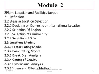
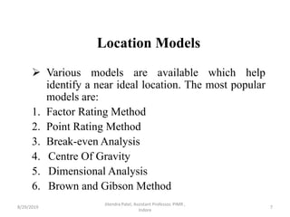
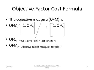
![• Location Measure
• LM= CFM x [D x OFM+ (1-D)x SFM]
• D(objective Factor Decision weight) =1- 0.40=0.60
8/29/2019 39
Jitendra Patel, Assistant Professor, PIMR ,
Indore](https://image.slidesharecdn.com/plantlocation-190829002323/85/Plant-location-39-320.jpg)
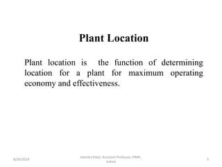
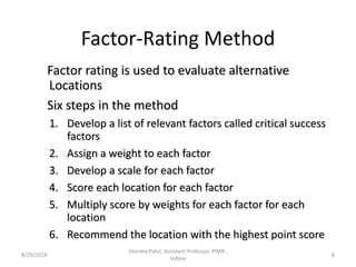
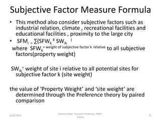
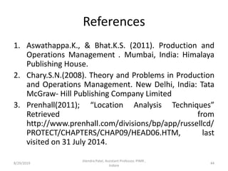
![LM Calculation for three Site
• Site 1
• LM= CFM x [D x OFM+ (1-D)x SFM]
= 1x[.60x 0.368+0.40 x0.194]
=0.2984
Site 2
= 1x[.60x 0.316+0.40 x0.431]
=0.3620
Site 3
=1x[.60x 0.316+0.40 x0.375]
=0.3396
Site 2 having highest Location Measure is preferred over other
two site.
8/29/2019 43
Jitendra Patel, Assistant Professor, PIMR ,
Indore](https://image.slidesharecdn.com/plantlocation-190829002323/85/Plant-location-43-320.jpg)


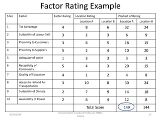
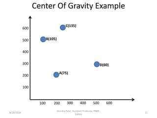
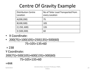
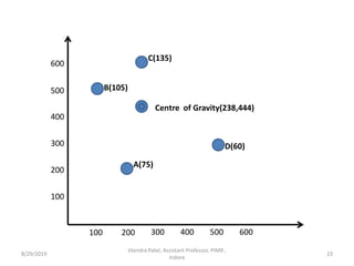
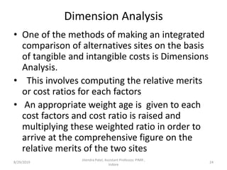
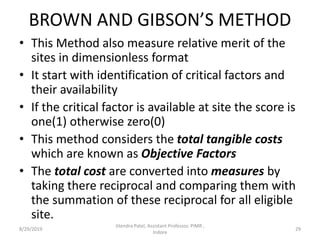
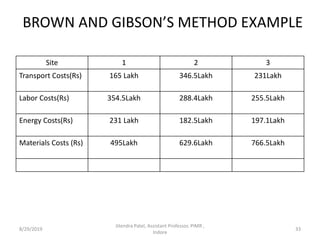
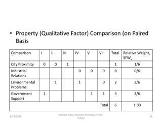
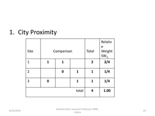
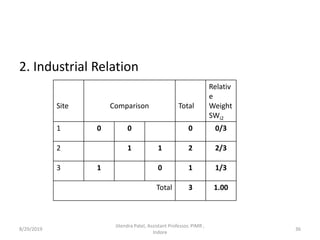
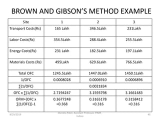
The document discusses various methods for selecting an optimal plant location, including factor rating, point rating, break-even analysis, center of gravity, and dimensional analysis. It provides examples of how to use each method, with the factor rating example comparing two locations based on weighted factors. Dimensional analysis is described as a way to integrate tangible and intangible costs by taking dimensionless ratios of costs and multiplying them with weightings. Brown and Gibson's method measures both objective factors based on costs and subjective factors to determine an overall location measure.


![Production & Operation Management Chapter30[1]](https://cdn.slidesharecdn.com/ss_thumbnails/chapter301-140613051722-phpapp02-thumbnail.jpg?width=640&height=640&fit=bounds)


