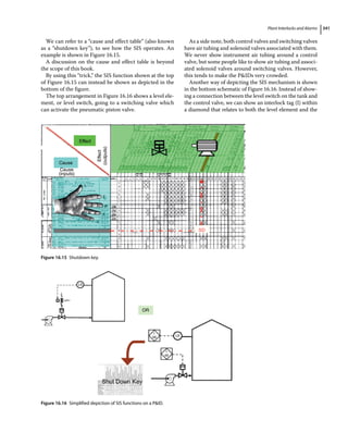
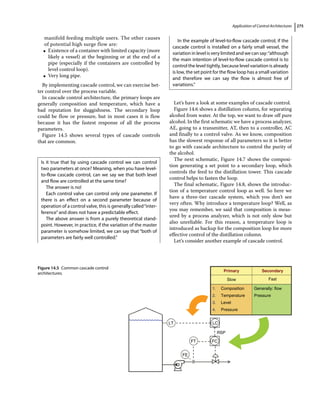
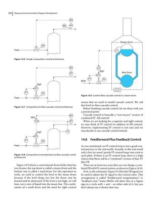
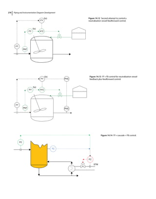
This document provides an overview of piping and instrumentation diagram (P&ID) development. It discusses the importance of P&IDs and the development process. Key parties involved in P&ID development include engineering, operations, and maintenance. The document also outlines the anatomy of a P&ID sheet and general rules for drawing P&IDs, including showing items, identifiers, and different types of diagrams. Principles of P&ID development include addressing normal and nonroutine operations as well as provisions for maintenance and future changes.

1. Piping and Instrumentation Diagram Development

2. Piping and Instrumentation Diagram Development
Moe Toghraei

3. This edition first published 2019
© 2019 John Wiley Sons, Inc.
A Joint Publication of the American Institute of Chemical Engineers and John Wiley Sons, Inc.
All rights reserved. No part of this publication may be reproduced, stored in a retrieval system, or transmitted, in any form or by any means,
electronic, mechanical, photocopying, recording or otherwise, except as permitted by law. Advice on how to obtain permission to reuse material
from this title is available at http://www.wiley.com/go/permissions.
Every effort has been made to ensure that the information in this course outline is accurate at the time of publication. Engrowth Training reserves
the right to modify content when necessary so that course content remains relevant.
No part of this course outline may be reproduced in any form or resold without written permission from Engrowth Training Inc., Alberta, Canada.
The rights of Moe Toghraei to be identified as the author of this work have been asserted in accordance with law.
Registered Office
John Wiley Sons, Inc., 111 River Street, Hoboken, NJ 07030, USA
Editorial Office
111 River Street, Hoboken, NJ 07030, USA
For details of our global editorial offices, customer services, and more information about Wiley products visit us at www.wiley.com.
Wiley also publishes its books in a variety of electronic formats and by print‐on‐demand. Some content that appears in standard print versions of
this book may not be available in other formats.
Limit of Liability/Disclaimer of Warranty
While the publisher and authors have used their best efforts in preparing this work, they make no representations or warranties with respect
to the accuracy or completeness of the contents of this work and specifically disclaim all warranties, including without limitation any implied
warranties of merchantability or fitness for a particular purpose. No warranty may be created or extended by sales representatives, written sales
materials or promotional statements for this work. The fact that an organization, website, or product is referred to in this work as a citation and/
or potential source of further information does not mean that the publisher and authors endorse the information or services the organization,
website, or product may provide or recommendations it may make. This work is sold with the understanding that the publisher is not engaged
in rendering professional services. The advice and strategies contained herein may not be suitable for your situation. You should consult with a
specialist where appropriate. Further, readers should be aware that websites listed in this work may have changed or disappeared between when
this work was written and when it is read. Neither the publisher nor authors shall be liable for any loss of profit or any other commercial damages,
including but not limited to special, incidental, consequential, or other damages.
Library of Congress Cataloging‐in‐Publication Data
Names: Toghraei, Moe, 1968– author.
Title: Piping and instrumentation diagram development / Moe Toghraei.
Description: First edition. | Hoboken, NJ, USA : John Wiley Sons, Inc., 2018. | Includes bibliographical references and index. |
Identifiers: LCCN 2018034188 (print) | LCCN 2018037545 (ebook) | ISBN 9781119329343 (Adobe PDF) | ISBN 9781119329831 (ePub) |
ISBN 9781119329336 (hardcover)
Subjects: LCSH: Chemical plants–Piping–Drawings. | Chemical apparatus–Drawings. | Blueprints.
Classification: LCC TP159.P5 (ebook) | LCC TP159.P5 T64 2018 (print) | DDC 621.8/6720222–dc23
LC record available at https://lccn.loc.gov/2018034188
Cover Design: Wiley
Cover Image: © tdub303/iStock.com
Set in 10/12pt Warnock by SPi Global, Pondicherry, India
Printed in the United States of America
10 9 8 7 6 5 4 3 2 1

4. ­
This book is dedicated to the soul of my father:
Behrouz

5. vii
Contents
Preface xix
Acknowledgement xxiii
About the Companion Website­ xxv
Part I Fundamentals of PID Development 1
1 What Is PID 3
1.1 ­
Why Is PID Important? 3
1.2 ­
What Is a PID? 4
1.3 ­PID Media 4
1.4 ­
PID Development Activity 5
2 Management of PID Development 9
2.1 ­
Project of Developing PIDs 9
2.2 ­PID Milestones 9
2.3 ­
Involved Parties in PID Development 11
2.4 ­
PID Set Owner 12
2.5 ­
Required Quality of the PID in Each Stage of Development 12
2.6 ­PID Evolution 12
2.7 ­
Tracking Changes in PIDs 12
2.8 ­
Required Man‐Hours for the Development of PIDs 13
3 Anatomy of a PID Sheet 15
3.1 ­Title Block 15
3.2 ­Ownership Block 15
3.3 ­
Reference Drawing Block 15
3.4 ­Revision Block 15
3.5 ­Comments Block 16
3.6 ­
Main Body of a PID 19
4 General Rules in Drawing of PIDs 21
4.1 ­Items on PIDs 21
4.1.1 Pipes or Other Flow Conductors 21
4.1.2 Equipment 21
4.1.3 Instruments 21
4.1.4 Signals 22
4.2 ­
How to Show Them: Visual Rules 22
4.2.1 Line Crossing Over 24
4.2.2 Equipment Crossing 25
4.2.3 Off‐Page Connector 26
4.2.4 Color in PIDs 26
4.3 ­
Item Identifiers in PIDs 26

6. Contents
viii
4.3.1 Symbols 27
4.3.2 Tags 28
4.3.3 Name 29
4.3.4 Technical Information 29
4.4 ­
Different Types of PIDs 32
4.4.1 Legend PIDs 33
4.4.2 System PIDs 34
4.4.3 Network PIDs 34
4.4.4 Interarea PIDs 34
4.4.5 Detail PIDs 36
4.5 ­
A Set of PIDs 39
4.6 ­
PIDs Prepared in Engineering Companies Compared to Manufacturing or Fabricating Companies 42
4.7 ­
Dealing with Vendor or Licensor PIDs 43
5 Principles of PID Development 45
5.1 ­Plant Stakeholders 45
5.2 ­
The Hierarchy of PID Development Rules 45
5.3 ­Plant Operations 46
5.3.1 Process Parameters 46
5.3.2 Process Parameter Levels 47
5.3.2.1 Pressure Levels 48
5.3.2.2 Temperature Levels 49
5.3.2.3 Liquid/Solid Levels 49
5.3.2.4 Flow Levels 50
5.3.2.5 Analyte Levels 50
5.3.3 Parameter Levels versus Control System 50
5.3.4 Parameter Levels versus Safety 51
5.3.5 Parameter Levels versus Operator Role 52
5.3.6 General Procedure of PID Development 53
5.4 ­
What Should a PID Address? 53
5.4.1 Normal Operation 53
5.4.2 Nonroutine Operation 53
5.4.2.1 Reduced Capacity Operation 54
5.4.3 Reduced Efficiency Operation 57
5.4.4 Start‐Up Operations 58
5.4.5 Shutdown 59
5.4.6 Inspection and Maintenance 60
5.4.6.1 Quantitative Approach to Maintenance Requirement 60
5.4.6.2 Qualitative Approach to Maintenance Requirement 60
5.4.7 Operability in Absence of One Item 61
5.4.8 Provision for the Future 61
5.5 ­
Conflicting Check and Merging Opportunities Check 63
5.5.1 Conflict Check 63
5.5.2 Merging Opportunities Check 63
5.6 ­
Dealing with Common Challenges in PID Development 64
5.7 ­
Example: Development of PID of a Typical Pump 65
Part II Pipes and Equipment 69
6 Pipes 71
6.1 ­
Fluid Conductors: Pipes, Tubes, and Ducts 71
6.2 ­Pipe Identifiers 71
6.2.1 Pipe Symbol 71
6.2.2 Pipe Tag 71

7. Contents ix
6.2.2.1 Do All Pipes Need to be Tagged? 73
6.2.2.2 Which Span of Pipe Route can be Considered
One Piece of Pipe? 73
6.2.2.3 How is the Pipe Tag Shown on a PID? 73
6.2.3 Pipe Off‐Page Connector 74
6.3 ­
Pipe Tag Anatomy 74
6.3.1 Area or Project Number 74
6.3.2 Commodity Acronym 74
6.3.3 Pipe Material Specification Code 74
6.3.4 Pipe Size 77
6.3.5 Pipe Sequential Number 78
6.3.6 Other Pipe Tag Information 78
6.4 ­
Pipes Crossing “Borders” 79
6.4.1 Implementing Spec Break 80
6.4.2 Reasons for a Spec Break 82
6.5 ­Goal of Piping 82
6.5.1 Magnitude of Flow in Pipe 83
6.5.2 Direction of Flow in Pipe 84
6.5.3 Providing Fluid with Enough Pressure at the Inlet 84
6.6 ­Piping Arrangements 84
6.6.1 Backflow Prevention Systems 85
6.6.2 Diversion of Flow 87
6.6.3 Distribution of Flow 87
6.7 ­Pipe Route 88
6.7.1 Slope 88
6.7.2 No Liquid Pocket 89
6.7.3 No Gas Pocket 89
6.7.4 Free Draining (Self‐Draining) 89
6.7.5 Free Venting 90
6.7.6 Gravity Flow 90
6.7.7 Vertical or Horizontal Pipe 90
6.7.8 Straight Piping 90
6.7.9 Minimum or Maximum Length or Distance 90
6.7.10 Other Special Pipe Routes 91
6.8 ­Piping Movement 91
6.9 ­
Dealing with Unwanted Two‐Phase Flow in Pipes 92
6.9.1 Liquid–Gas Two‐Phase Flow 92
6.9.2 Gas–Liquid Two‐Phase Flow 94
6.9.3 Solid–Liquid Two‐Phase Flow 94
6.10 ­Tubes 94
6.11 ­Double–Wall Pipes 95
6.12 ­
Pipes for Special Arrangements 96
6.12.1 Piping for Bypassing 96
6.12.2 Piping for Recirculation 96
6.12.3 Piping for Units in Series 96
6.12.4 Piping for Units in Parallel 97
6.12.5 Piping for Pressure Equalization 97
6.13 ­
Pipe Size Rule of Thumbs 97
6.14 ­Pipe Appurtenances 97
6.14.1 Pipe Fittings 98
6.14.1.1 Pipe Direction Change 98
6.14.1.2 Reducers (Enlargers) 98
6.14.1.3 Three‐Way Connections 100
6.14.1.4 Pipe Connections 100
6.14.1.5 End‐of‐Pipe Systems 100

8. Contents
x
6.14.2 Specialty Items 102
6.14.2.1 Flange‐Insulating Gasket 102
6.15 ­
Other Approach about Piping 103
6.16 ­“Merging” Pipes 103
6.17 ­
Wrapping–Up: Addressing Requirements of Pipe during the Life Span 103
6.18 ­
Transferring Bulk Solid Materials 104
­ Reference 104
7 Manual Valves and Automatic Valves 105
7.1 ­Valve Naming 105
7.2 ­Valve Functions 105
7.3 ­Valve Structure 105
7.4 ­Classification of Valves 105
7.4.1 Valve Plug: Throttling vs. Blocking Valves 106
7.4.2 Valve Selection 108
7.4.3 Multi‐port Valves 108
7.4.4 Double‐Seated Valves 110
7.5 ­Valve Operators 110
7.6 ­
Different Types of Actuators 111
7.7 ­
Basis of Operation for Automatic Valves 112
7.8 ­
Tagging Automatic Valves 113
7.9 ­
Tagging Manual Valves 113
7.10 ­Valve Positions 113
7.10.1 Regular Position of Blocking Valves and Decision Methodology 113
7.10.2 Failure Position of Automatic Valves and Decision Methodology 114
7.10.3 More Concepts about Failure Position of Automatic Valves 115
7.11 ­Valve Arrangement 117
7.11.1 Valves in Series 118
7.11.2 Valves in Parallel 118
7.12 ­
Control Valves and RO Combinations 119
7.13 ­
Operating in the Absence of Valves 119
7.13.1 Operating in the Absence of Control Valves 119
7.13.2 Operating in the Absence of Switching Valves 122
7.14 ­
Valves in Role of Unit Operation 122
7.15 ­Special Valves 123
7.15.1 Check Valves 123
7.15.2 Regulators 124
7.15.3 Safety‐Related Valves 125
7.16 ­Valve Combinations 126
7.17 ­
End of Valve Arrangements 126
7.18 ­
Valve Sizing Rule of Thumbs 127
7.19 ­Merging Valves 127
7.20 ­
Wrapping Up: Addressing Requirements of Valve During the Life Span 127
­ References 128
8 Provisions for Ease of Maintenance 129
8.1 ­Introduction 129
8.2 ­
Different Types of Equipment Care 129
8.3 ­
In‐place In‐line Equipment Care 129
8.4 ­
In‐place Off‐line Equipment Care 130
8.5 ­
In‐workshop Off‐line Equipment Care 131
8.6 ­
Preparing Equipment for Off‐line Care 131
8.7 ­Isolation 131
8.7.1 Requirement of an Isolation System 131

9. Contents xi
8.7.2 Type of Isolation System 132
8.7.3 Placement of an Isolation System 135
8.7.4 Inbound Versus Outbound Blind Location 135
8.7.5 Merging Isolation Valves 135
8.8 ­
Bringing the Equipment to a Non‐harmful Condition 136
8.8.1 Cooling Down 136
8.8.2 Emptying and Then Draining/Venting 136
8.8.2.1 Location and Number of Drain/Vent Valves 137
8.8.2.2 Size of Drain/Vent Valves 138
8.8.2.3 Other Usages of Drain/Vent Valves 138
8.9 ­Cleaning 139
8.9.1 Solid/Semi‐Solid Removal Methods 139
8.9.2 Washing Systems 139
8.9.3 Purging Methods 140
8.10 ­
Ultimate Destination of Dirty Fluids 140
8.11 ­
Making Equipment Easy to Remove 141
8.12 ­Wrap‐up 142
9 Containers 143
9.1 ­Introduction 143
9.2 ­Selection of Containers 143
9.3 ­Containers Purposes 144
9.4 ­
Transferring Fluids Between Containers 145
9.5 ­Container Positions 146
9.6 ­Container Shapes 147
9.6.1 Closing Parts of Containers 148
9.6.2 Open Top or Fully Enclosed Containers 148
9.7 ­Container Identifiers 148
9.7.1 Container Symbol 148
9.7.2 Container Tags 149
9.7.3 Container Call‐outs 149
9.7.3.1 Tank Call‐outs 149
9.7.3.2 Vessel Call‐outs 150
9.7.3.3 Tag of Container in Duty of Conversion 151
9.8 ­
Levels in Non‐flooded Liquid Containers 151
9.9 ­Container Nozzles 151
9.9.1 Nozzle Duties 151
9.9.2 Nozzle Locations 152
9.9.3 Nozzle Elevation Versus Liquid Levels 153
9.9.4 The Size, Number, and Rating of Nozzles 155
9.9.5 Merging Nozzles 155
9.9.6 Nozzle Internal Assemblies 156
9.9.7 Nozzle Externals 157
9.10 ­Overflow Nozzles 157
9.11 ­
Breathing of Non‐flooded Containers 158
9.12 ­Blanketed Tanks 160
9.13 ­
Heating (or Cooling) in Containers 161
9.14 ­Mixing in Containers 162
9.15 ­Container Internals 162
9.16 ­Tank Roofs 162
9.17 ­Tank Floors 163
9.18 ­Container Arrangement 164
9.19 ­Merging Containers 164
9.20 ­Secondary Containment 165

10. Contents
xii
9.21 ­
Underground Storage Tanks 166
9.22 ­Sumps 167
9.23 ­
Wrapping‐up: Addressing the Requirements of the Container During its Lifespan 167
10 Pumps and Compressors 169
10.1 ­Introduction 169
10.2 ­
Fluid Mover Roles 169
10.3 ­
Types of Fluid Movers 169
10.4 ­
A Brief Discussion on the Function of Fluid Movers in a System 169
10.5 ­
Fluid Mover Identifiers 171
10.5.1 Fluid Mover Symbol 171
10.5.2 Fluid Mover Tag 171
10.5.3 Fluid Mover Call‐out 173
10.6 ­
Liquid Movers: Dynamic Pumps 173
10.6.1 Centrifugal Pumps 173
10.6.1.1 PID Development on the Suction Side 174
10.6.1.2 PID Development on the Discharge Side 175
10.6.2 Low Flow Intolerance and Minimum Flow Protection System 176
10.6.2.1 Which Pumps May Need a Minimum Flow Pipe 176
10.6.2.2 Where Should we Position the Recirculation Line? 177
10.6.2.3 Where Should the Destination Point of the Recirculation Pipe Be? 177
10.6.2.4 What Should the Size of the Recirculation Pipe Be? 178
10.6.2.5 What Should the Arrangement on the Recirculation Pipe Be? 178
10.6.3 Cavitation 180
10.6.4 Very Small Centrifugal Pumps 181
10.6.5 Different Types of Spare Pump 182
10.6.6 Centrifugal Pump Arrangements 182
10.6.6.1 Centrifugal Pumps in Parallel 183
10.6.6.2 Centrifugal Pumps in Series 184
10.6.7 Pump Warm‐up or Cool‐down System 185
10.6.8 Piping Spec. for Centrifugal Pumps 187
10.6.9 Centrifugal Pump Drives 187
10.6.10 (Liquid) Seal Systems in Centrifugal Pumps 187
10.6.11 Merging Pumps 189
10.7 ­
Liquid Movers: PD Pumps 190
10.7.1 PD Pump PID Piping 191
10.7.1.1 Reciprocating Pumps PID Piping 191
10.7.1.2 Rotary Pumps PID Piping 192
10.7.2 PD Pump Arrangements 193
10.7.3 Merging PD Pumps 193
10.7.4 Tying Together Dissimilar Pumps 193
10.7.5 PD Pump Drives 193
10.7.6 Sealing Systems for PD Pumps 194
10.7.7 Metering Pumps (Dosing Pumps) 194
10.7.8 Liquid Transfer – Summary 195
10.7.9 Pumps: Duty Other than Pumping! 195
10.8 ­
Gas Movers: Fans, Blowers, Compressors 196
10.8.1 Low Flow Intolerance and Anti‐Surge Systems 196
10.8.2 PID Development of Gas Movers 197
10.8.3 Gas Mover Drives 198
10.8.4 Auxiliary Systems Around Fluid Movers 198
10.8.5 Gas Transfer – Summary 199
10.9 ­
Wrapping‐up: Addressing Requirements of Fluid Movers During the Life Span 200
Reference 200

11. Contents xiii
11 Heat Transfer Units 201
11.1 ­Introduction 201
11.2 ­
Main Types of Heat Transfer Units 201
11.3 ­
Different Types of Heat Exchangers and Their Selection 202
11.4 ­
Different Types of Heat Transfer Fluids and Their Selection 203
11.5 ­
Heat Exchangers: General Naming 204
11.6 ­
Heat Exchanger Identifiers 204
11.6.1 Heat Exchanger Symbol 204
11.6.2 Heat Exchanger Tag 204
11.6.3 Heat Exchanger Call‐Out 205
11.7 ­
Heat Exchanger PID 206
11.7.1 Vents and Drains 206
11.7.2 Isolation Valves 207
11.7.3 Chemical Cleaning Valves 207
11.7.4 PSDs 207
11.8 ­
Heat Exchanger Arrangement 207
11.8.1 Heat Exchangers in Series 207
11.8.2 Heat Exchangers in Parallel 209
11.9 ­Aerial Coolers 209
11.9.1 Aerial Cooler PID 210
11.9.2 Dealing with Extreme Temperatures 211
11.9.3 Aerial Cooler Arrangement 211
11.10 ­
Merging Heat Exchangers 212
11.11 ­
Wrapping‐up: Addressing the Requirements of a Heat Exchanger During its
Life Span 212
11.12 ­
Fired Heaters and Furnaces 213
11.12.1 Process Fluid Side 213
11.12.2 Flue Gas Side 213
11.12.3 Firing Side 214
11.13 ­
Fire Heater Arrangement 215
11.14 ­
Merging Fired Heaters 216
11.15 ­
Wrapping‐up: Addressing the Requirements of Fired Heaters During their Lifespan 216
12 Pressure Relief Devices 217
12.1 ­Introduction 217
12.2 ­
Why Pressure Is So Important? 217
12.3 ­
Dealing with Abnormal Pressures 217
12.3.1 Active Versus Passive Solutions 219
12.3.2 Where Could Passive Solutions Be Used? 219
12.3.3 Where Should Active Solutions Be Used? 219
12.4 ­
Safety Relief System 219
12.5 ­
What Is an “Enclosure,” and Which “Side” Should Be Protected? 220
12.6 ­
Regulatory Issues Involved in PRVs 220
12.6.1 Codes Versus Standards 221
12.7 ­PRD Structure 222
12.8 ­
Six Steps to Providing a Protective Layer 222
12.9 ­Locating PRDs 223
12.10 ­Positioning PRDs 223
12.11 ­Specifying the PRD 225
12.12 ­
Selecting the Right Type of PRD 225
12.12.1 Pressure Relief Valve Type 225
12.12.2 Rupture Disks 226
12.12.3 Decision General Rules 226
12.13 ­PRD Identifiers 226

12. Contents
xiv
12.13.1 PRD Symbols and Tags 226
12.13.2 PRD Technical Information 227
12.14 ­
Selecting the Right Type of PRD Arrangement 228
12.15 ­
Deciding on an Emergency Release Collecting Network 230
12.16 ­
Deciding on a Disposal System 232
12.16.1 Liquid Disposal 232
12.16.2 Gas/Vapor Disposal 233
12.16.3 Two‐Phase Flow Handling 234
12.17 ­
Protecting Atmospheric Containers 235
12.18 ­Merging PRDs 236
12.19 ­
Wrapping‐Up: Addressing the Requirements of PRDs During their Lifespan 238
Part III Instrumentation and Control System 239
13 Fundamentals of Instrumentation and Control 241
13.1 ­
What Is Process Control? 241
13.2 ­
Components of Process Control Against Violating Parameters 241
13.3 ­
Parameters Versus Steering/Protecting Components 242
13.4 ­
How Many Steering Loops Are Needed? 242
13.5 ­
ICSS System Technology 243
13.5.1 Use of PLC for a BPCS 243
13.5.2 Use of DCS for a SIS 244
13.5.3 Alarm Systems 244
13.5.4 ICSS System Symbology 244
13.6 ­ICSS Elements 245
13.7 ­
Basic Process Control System (BPCS) 245
13.8 ­Instruments on PIDs 247
13.8.1 Fundamental Terminology 247
13.8.2 Identifiers for Equipment and Instrumentation 247
13.9 ­Instrument Identifiers 248
13.9.1 Acronyms 248
13.9.2 Divider Types 249
13.9.3 Symbol Type 250
13.9.4 Additional Information and Tag Number 252
13.10 ­
Signals: Communication Between Instruments 252
13.10.1 Signal Types 253
13.10.2 Signal Functions 253
13.10.3 Signal Math Functions 254
13.10.4 Signal Selectors 254
13.11 ­
Different Instrument Elements 255
13.11.1 Primary Instruments 255
13.11.1.1 Temperature Measurement 256
13.11.1.2 Pressure Measurement 257
13.11.1.3 Level Measurement 258
13.11.1.4 Flow Measurement 258
13.11.1.5 Process Analyzers 260
13.11.2 Transmitters 262
13.11.3 Controllers 263
13.11.4 Indicators 263
13.11.5 Final Control Elements in a BPCS 263
13.11.5.1 Control Valves 264
13.11.5.2 Variable Speed Devices on Electric Motors 264
13.12 ­
Simple Control Loops 264

13. Contents xv
13.12.1 Level Control Loops 265
13.12.2 Pressure Control Loops 265
13.12.3 Temperature Control Loops 265
13.12.4 Composition Control Loops 266
13.12.5 Flow Control Loops 266
13.13 ­
Position of Sensor Regarding Control Valves 266
14 Application of Control Architectures 269
14.1 ­Introduction 269
14.2 ­
Control System Design 269
14.3 ­
Selecting the Parameter to Control 269
14.4 ­
Identifying the Manipulated Stream 270
14.5 ­
Determining the Set Point 271
14.6 ­
Building a Control Loop 272
14.6.1 Feedback Versus Feedforward 272
14.6.2 Single‐ versus Multiple‐Loop Control 273
14.7 ­
Multi‐Loop Control Architectures 274
14.7.1 Cascade Control 274
14.8 ­
Feedforward Plus Feedback Control 276
14.8.1 Ratio or Relationship Control 279
14.8.2 Selective Control 280
14.8.3 Override and Limit Control 281
14.8.3.1 Override Control 283
14.8.3.2 Limit Control 286
14.8.4 Split Range and Parallel Control 286
14.8.5 Clarification of Confusion 288
14.8.5.1 Cascade Versus Ratio 288
14.8.5.2 Single Loop Versus Ratio 288
14.8.5.3 Selective Versus Override 288
14.9 ­Monitoring Parameters 289
14.9.1 Container Sensors 290
14.9.2 Fluid Mover Sensors 290
14.9.3 Heat Exchanger Sensors 291
14.9.4 Fired Heater Sensors 291
15 Plant Process Control 293
15.1 ­Introduction 293
15.2 ­Plant‐Wide Control 293
15.3 ­
Heat and Mass Balance Control 293
15.4 ­Surge Control 295
15.4.1 Disturbances in Process Parameters 295
15.4.2 Disturbance Management 296
15.4.2.1 Absorption 296
15.4.2.2 Rejection 296
15.4.3 Disturbance Versus Fluid Phase 296
15.4.4 Dampening Gas/Vapor Flow Surge 297
15.4.5 Dampening Liquid Flow Surge 298
15.4.6 The Purpose of Containers in Process Plants 301
15.5 ­Equipment Control 302
15.5.1 Do We Need to Control at All? 302
15.5.2 Principles of Equipment‐wise Control 302
15.6 ­
Pipe Control System 304
15.6.1 Control of a Single Pipe 304
15.6.1.1 Control of Pressure in a Pipe 304

14. Contents
xvi
15.6.1.2 Control of Flow in a Pipe 304
15.6.2 Controlling Multiple Pipes 306
15.6.2.1 Flow Merging 306
15.6.2.2 Flow Splitting 308
15.7 ­
Fluid Mover Control System 309
15.7.1 Pump Control Systems 310
15.7.1.1 Centrifugal Pump Control 310
15.7.1.2 Positive Displacement (PD) Pump 314
15.7.2 Gas Mover Control Systems 316
15.7.2.1 Capacity Control Methods for Gas Movers 316
15.7.3 Anti‐Surge Control 319
15.7.4 Lead–Lag Operation of Fluid‐Movers 319
15.8 ­
Heat Transfer Equipment Control 320
15.8.1 Heat Exchanger Control System 320
15.8.1.1 Direct Control System 320
15.8.1.2 Bypass Control System 321
15.8.1.3 Control of Heat Exchangers Experiencing Phase Change 324
15.8.2 Air Cooler Control 327
15.8.3 Heat Exchanger for Heat Recovery 327
15.8.4 Back Pressure Control of Heat Exchangers 328
15.8.5 Fired Heater Control 328
15.9 ­
Container Control System 331
15.10 ­
Blanket Gas Control Systems 332
Reference 332
16 Plant Interlocks and Alarms 333
16.1 ­Introduction 333
16.2 ­Safety Strategies 333
16.3 ­Concept of a SIS 333
16.4 ­
SIS Actions and SIS Types 333
16.5 ­SIS Extent 336
16.6 ­
Deciding on the Required SIS 336
16.7 ­
The Anatomy of a SIS 336
16.7.1 SIS Element Symbols 336
16.7.1.1 SIS Primary Elements: Sensors 337
16.7.2 SIS Final Elements 337
16.7.2.1 Switching Valves 337
16.7.2.2 Switching Valve Actuator Arrangements 338
16.7.2.3 Valve Position Validation 338
16.7.2.4 Merging a Switching Valve and a Control Valve 338
16.7.2.5 On/off Action of Electric Motors 339
16.7.3 SIS Logic 339
16.8 ­
Showing Safety Instrumented Functions on PIDs 340
16.9 ­Discrete Control 343
16.10 ­Alarm System 344
16.10.1 Anatomy of Alarm Systems 345
16.10.2 Alarm Requirements 345
16.10.3 Alarm System Symbology 346
16.10.4 Concept of “Common Alarm” 347
16.11 ­
Fire and Gas Detection System (FGS) 347
16.11.1 Manual Alarm 350
16.12 ­
Electric Motor Control 351
16.12.1 Simple Motor Control 351
16.12.2 The Focal Element of Motor Control: MCC 351

15. Contents xvii
16.12.3 All About Relationships with Electric Motors 351
16.12.4 PID Representation of Commands and Responses 352
16.12.5 PID Representation of Principal Arrangement for Inspection and Repair 353
16.12.6 Examples 355
Part IV Utilities 357
17 Utilities 359
17.1 ­
Utility System Components 359
17.2 ­
Developing PIDs for Utility Systems 359
17.2.1 Identifying the Utility Users 359
17.2.2 Utility Distribution and Collection Network Topologies 359
17.2.3 Designing the Detail of a Utility Network 361
17.2.4 Placing Priority on Utility Users 362
17.2.5 Connection Details of Utility to Process 363
17.3 ­
Different Utilities in Plants 363
17.4 ­
Air as a Utility in Process Plants 363
17.4.1 Instrument Air (IA) 363
17.4.2 Utility Air (UA) or Plant Air (PA) 364
17.5 ­
Water as a Utility in Process Plants 364
17.5.1 Utility Water (UW) or Plant Water (PW) 364
17.5.2 Potable Water 364
17.6 ­
Heat Transfer Media 364
17.6.1 Steam 365
17.7 ­
Condensate Collection Network 366
17.8 ­Fuel as Utility 366
17.8.1 Fuel Oil 366
17.8.2 Fuel Gas 366
17.9 ­Inert Gas 367
17.9.1 Blanket Gas 367
17.9.2 Purging Gas 367
17.10 ­
Vapor Collection Network 367
17.11 ­
Emergency Vapor/Gas Release Collection Network 368
17.12 ­Fire Water 368
17.13 ­
Surface Drainage Collection Network or Sewer System 370
17.14 ­Utility Circuits 372
17.14.1 Air Circuit 372
17.14.2 Steam–Condensate Circuit 374
17.14.3 Cooling Water Circuit 375
17.14.4 Natural Gas Preparation System 375
17.15 ­
Connection Between Distribution and Collecting Networks 375
Part V Additional Information and General Procedure 379
18 Ancillary Systems and Additional Considerations 381
18.1 ­Introduction 381
18.2 ­Safety Issues 381
18.2.1 Different Types of Hazards 381
18.2.2 Hazards and Injuries 381
18.2.3 Mechanical Hazards 381
18.2.4 Chemical Hazards 382
18.2.5 Energy Hazards 382

16. Contents
xviii
18.2.5.1 Noise Barrier 382
18.2.5.2 Burning Prevention 382
18.2.6 Safety Showers and Eye Washers 383
18.3 ­Dealing with Environment 384
18.3.1 Arrangements for Maintaining the Temperature of the Process 384
18.3.2 Winterization 385
18.3.3 Deciding on the Extent of Insulation 389
18.3.4 Summary of Insulation 390
18.4 ­Utility Stations 390
18.5 ­
Off‐Line Monitoring Programs 392
18.5.1 The Program Component 392
18.5.2 Sampling System 393
18.5.3 Sample Extraction Device 393
18.5.4 Sample Transferring Tube 394
18.5.5 Sample Conditioning System 394
18.5.6 Sample Hand‐Over System 395
18.5.7 Waste Sample Collection System 395
18.5.8 Sampling Station Structural Frame 395
18.5.9 Showing a Sampling System on PIDs 396
18.5.10 Sampling System for Process Analyzers 396
18.6 ­
Corrosion Monitoring Program 396
18.7 ­
Impact of the Plant Model on the PID 397
18.8 ­
Design Pressure and Temperature Considerations 398
18.8.1 Decision on “Design Pressure @ Design Temperature” Pair 399
18.8.1.1 Deciding on “Design Pressure” 399
18.8.1.2 Deciding on “Design Temperature” 399
18.8.2 Sources of Rebel Pressures 400
18.8.3 Sources of Rebel Temperatures 400
18.8.4 Design Pressure and Design Temperature of Single Process Elements 400
18.8.5 Design Pressure of Connected Items 401
18.8.5.1 Design Pressure of Connected Equipment–Equipment 402
18.8.5.2 Design Pressure of Connected Equipment–Sensor 403
19 General Procedures 405
19.1 ­Introduction 405
19.2 ­
General Procedure for PID Development 405
19.2.1 PID Development: Piping and Equipment 405
19.2.2 PID Development: Control and Instruments 406
19.3 ­
PID Reviewing and Checking 409
19.3.1 Format Check 409
19.3.2 Demonstration Rules Check 410
19.3.3 Technical Check 410
19.3.4 Design Check 412
19.4 ­
Methods of PID Reviewing and Checking 412
19.4.1 Systematic Approach 412
19.4.2 Scanning Approach 412
19.5 ­
Required Quality of PIDs at Each Stage of Development 413
20 Examples 417
Index 453

17. xix
The need for a book on piping and instrument diagram
(PID) development is always felt in the process indus-
tries. However, for a long time there no book covered
this topic.
There are several reasons for this.
One reason is the practical nature of this skill. A large
number of books written for working professionals are
authored by university professors. The skill of PID
development however is not pure theoretical knowledge.
It is a combination of technical skills and other considera-
tions like ease of operation, ease of maintenance, client
preferences, and jurisdictional codes.
On the other hand, the required technical skill is not
exclusively in the territory of chemical engineers or
instruments/control engineers or any other single
engineering discipline. The set of skills for PID devel-
opment comes from different engineering disciplines.
Because of the above issues, the PID development
skill is always considered as an “on the job learning” skill.
The roadblocks of a book on PID development are
not only the vastness of the skill or the practical nature of
it, but also some preventing beliefs.
Some people claim that PID drawing is similar to a
painting, which involves a bunch of creativity. Therefore
“PID development” cannot be taught. However, the
answer is in their question: even though painting needs a
bunch of creativity it doesn’t prevent teachers/instruc-
tors from writing books to explain the fundamentals of
painting and also showing some of the creativities by
other painters to spur the learner’s creativity.
Some other people claim that PID development can
be done only by following the company guidelines and
such a topic cannot be taught as a general course.
However, all the instructions in the company’s guidelines
have underlying logic. This book tries to explain these
logical backgrounds.
The goal of this book is to provide information about
the development of PIDs for designers and personnel
of process plants.
When it comes to PID, there are three main group of
knowledge may come to mind. They are:
1) The group of information on the technical “develop-
ment” of PIDs
2) The group of information that shows different ele-
ments on PID sheets
3) The group of information about how to draw already‐
developed PIDs (drafting PIDs).
A PID should first be developed (step 1), then drafted
(step 3) based on the rules of PID appearance (step2).
This concept is shown in the diagram.
Developing PID Drafting PID
This book doesn’t address how to “draw” a PID
(group 3). There is plenty of software and plenty of train-
ing courses by the software companies that cover that
topic.
This book mainly focuses on the development of
PIDs and how to show different elements on PIDs.
The information in this book will not only help in the
development of PIDs, but will also help in under-
standing the activities of process plants that are related
to PIDs.
Chemical engineers will use this book to learn how to
design process plants based on selected and designed/
specified equipment or unit operations or process units.
They will learn how to “tie” together different units to
make sure the plant runs safely and produces the prede-
termined products with the highest level of operability.
Chemical engineers and other engineers in process
plants will use this book so that they can read and inter-
pret PIDs deeply in order to maintain any piece of
equipment in the plant and/or doing repair.
There are several disciplines involved, including chem-
ical engineering, mechanical, piping instrumentation
and control, electrical engineering, and civil engineering
disciplines.
All disciplines involving a process plant should be
familiar with PIDs.
Preface

18. Preface
xx
Since the PID is a multidisciplinary drawing, the con-
cepts must be presented in layman’s terms in order to be
accessible to a wide range of engineers. As it has been seen
that individuals with different level of study, from engi-
neers to technologists and technicians, have the duty of
PID development, this book is written for whoever has
enough knowledge of process plants and wants to learn
PID development skills. Therefore the concepts are not
necessarily explained in university level language.
The skeleton of this book has five parts as below.
Part 1: Fundamentals of PID Development
This part covers the fundamentals of PIDs and PID
development. Chapters 1 to 5 comprise Part 1 of this book.
At the beginning I will explain the nature and impor-
tance of PIDs (Chapter 1). Then I will explain the mile-
stones in developing PIDs (Chapter 2). In Chapter 3
the “court of game”, or different sections of a PID sheet
will be explained. In Chapter 4, the basic rules of draft-
ing PIDs will be discussed. Chapter 5 talks about the
thought process for developing PIDs and what goals a
designer needs to look for to develop a good PID.
When talking about “piping and instrumentation
diagrams” it seems the topic can be explained by explaining
two elements of piping (and equipment) and instrumenta-
tion. However for different reasons I have decided to
divide the topic into the three elements of pipes and
equipment, instrumentation/control systems, and utility
generation and networks.
Part 2 is devoted to pipes and equipment, Part 3 will
cover instrumentation and control systems, and Part 4
covers topics related to utilities.
For each of these elements the skills for PID develop-
ment is explained together with plenty of general prac-
tices for each component.
Part 2: Pipes and Equipment
The majority of process items (pipes and equipment)
in different PIDs are pipes and pipe appurtenances,
valves (manual and automatic), containers (tanks and
vessels), fluid movers (including pump, compressor, fan,
and blower), and heat exchangers.
Part 2 has seven chapters. In Chapter 6, pipe and pipe
fittings are discussed. Chapter 7 belongs to different
types of valves.
Chapter 8 provides information about the develop-
ment of PIDs considering inspection and maintenance.
As such provision needs to be made for specific types of
pipe and valve arrangement and this topic is placed after
Chapter 6.
Chapter 9 discuss different types of containers includ-
ing tanks and vessels and the way we develop their
PIDs.
Chapter 10 covers fluid movers. Fluid movers include
liquid movers or pumps and gas/vapor movers or com-
pressors, blowers, and fans.
Chapter 11 talks about heat transfer units. They are
mainly divided into heat exchangers and furnaces (fired
heaters).
Pressure safety devices (PSDs) are discussed in
Chapter 12. Although one main portion of PSDs are
pressure safety valves (PSVs), and are a special type of
valves, it was decided to devote a separate chapter to
them. The reason is that another portion of PSD is rup-
ture disks, which are not a type of valve, and also the con-
cept of PSDs is adequately important to consider a
separate chapter for them.
Part 3: Instrumentation and Control
Part 3 comprises the four Chapters of 13, 14, 15, and 16.
Chapter 13 developed to give a basic practical idea
about instrumentation and control to the reader. As is
mentioned there, the control system, or in a more com-
plete phrase integrated control and safety, in each plant
has three main elements.
In Chapter 14 the concept of control loop and the
method of developing control loops on PID are
discussed.
The first element of control is covered in Chapter 14 as
“plant control”. The other two elements, interlock and
alarm systems are covered in Chapters 15 and 16.
Part 4: Utilities
In Chapter 17, the reader will learn about utility sys-
tems in a process plant and how to develop their PIDs.
When talking about utilities, there are two separate con-
cepts that should be discussed: utility generation and
then the distribution of utilities and the collection of
“used” utilities. Both of them are discussed in this
chapter.
Part 5: Additional Information and Wrap‐up
Part 5 covers additional information to that covered in
the previous chapters. Part 5 has two chapters, Chapters
17 and 18.
Chapter 17 covers some additional small systems
(tracing and insulation, utility stations, safety showers
and eye washers, sampling systems, and corrosion
coupons) and also an important topic that is very impor-
tant in PID development.
The important topic, covered as part of chapter 17, is
“design pressure and temperature considerations”. This
topic covers precautions should be taken when tying
together different process elements in PIDs.
In chapter 18 some units that could be categorized in
the previous chapters are presented. The important con-
cept of design temperature and design pressure is also
studied here.
Chapter 19 could be considered as summary of the
previous chapters. In this chapter a general methodology
is provided for PID development of a new item (not
familiar for the designer) and then PID development of
some common systems (like chemical injection system,

19. Preface xxi
silo and solid transfer, etc.) is brought. At the end PID
reviewing and checking is discussed.
Introduction: What is PID Development Skill?
The first thing is to decide is the meaning of PID
development. The answer can be prepared regarding two
aspects: the depth and the breadth.
All the items on a PID sheet went through two steps
and several engineering disciplines. The depth of PID
development could be defined as all activities to develop
a PID but beyond the design.
The breadth of PID development could be defined as
all activities by different engineering disciplines.
The depth of PID development is explained in more
detail below.
Each discipline does the design and then PID
development.
The design, in this context, means sizing or specifying
a piece of an element such as a pipe, equipment, instru-
ment, etc.
There are different disciplines involved in the design
of a process plant, including process engineering,
­
piping and piping engineering, instrumentation and
control engineering, mechanical engineering, and civil
engineering.
The duties of the chemical engineer in a CPI project
can be broadly split into two categories: equipment sizing/
specification and PID development. Therefore the
chemical engineer needs to have skills in both classes.
The former skill needs primarily knowledge of hydrau-
lic calculations, pump/compressor sizing, vessel/tank
sizing, PSV sizing, and heat exchanger sizing. At a higher
level of sizing skill the chemical engineer should have the
knowledge of designing different unit operation and unit
processes. For example an engineer in the air purifica-
tion industry may need to know about the design of
different solid–gas separation units. Another engineer in
the oil refining industry may need to know how to size a
distillation tower. All of these sizing skills could have
been learned during the acquisition of an engineering
degree.
However, the latter—which is not formally taught and
considered as “on the job” learning—includes the skills
required to determine appropriate piping, piping appur-
tenances, proper tanks, vessels, pumps, and also instru-
mentation/control to determine the goal of the plant.
Equipment sizing is beyond the scope of this book.
However, sometimes it is not easy to put a separation line
between equipment sizing and PID development. The
result of equipment sizing AND PID development
effort makes PIDs.
Sizing or
specification
PID
development
PID
Some concepts in this book may be considered as
sizing skill concepts by some individuals but they are still
included in the book. The reason is that a PID docu-
ment could be used to “check” the sizing during the
PID development stage. As a PID gives a big picture
of a plant, sometimes the mistakes in equipment sizing
could be revealed when the equipment appears on the
PID. Therefore, some of the concepts in this book can
be used to “roughly” check the accuracy of sizing of pipes
and equipment.
The breadth of PID development is explained in
more detail below.
The question is: which sector of PID skills are out-
linedhere?Chemicalengineeringsector?Instrumentation
and control sector? Mechanical engineering sector?
As was mentioned before, PID development skills
are stretched over multiple disciplines. A PID sheet is
the result of exhaustive work by different disciplines.
Each item on a PID may be rooted in a deep concept of
chemical engineering, instrumentation and control engi-
neering, mechanical engineering, etc.
PID development
Process
Control
Operation
Equipments
Instruments
Location
Regulations:
HSE
Maintenance
Supporting
plants
At the beginning of PID development the items are
added on PIDs based on some calculations and sizing.
However, when we progress further, the added items on
PIDs are not backed by quantitative documents but by
qualitative, judgment‐type decisions.
Calculation
Technical Not technical
PID
development
The content of this book covers not only the chemical
engineering sector of PID development but also the
required knowledge of other disciples to develop PIDs
is covered.

20. Preface
xxii
This book, however, doesn’t eliminate the need for
professionals in different areas because it only provides
some rule of thumbs in those areas to help and accelerate
the developing of PIDs.
No attempt was made to explain the deep concepts, as
they are discussed in other books with better depth and
breadth. This is the reason that there are few references
in each chapter because I try to convey only the skill of
PID development.
Therefore, this book can be considered as book of rules of
thumb for PID development. The readers learn the “root”
of knowledge needed to refer to the respective resources.

21. xxiii
In preparing this book I indebted to many professionals
who have helped me. Amongst them, I acknowledge
assistance of Dr. Ashgar Mesbah for his helpful notes on
Chapter 13, Greg Pajak for his consultation to provide a
better content in chapter 16. I am also very grateful my
old fried, Shahriar Gilanmorad for accepting to develop
and draw many schematics of this book.
I also must acknowledge all the helpful guidance and
help I received from Rasoul Sayedin during my career
and regarding PID development.
Finally, to my wife, Mishga Abedin, who suffered but
supported me through the writing of this book.
At the end, I will appreciate it very much if all profes-
sionals who use this book let me know of any errors
which is made or any change, they believe needed to
improve the book.
Moe Toghraei
Calgary, Alberta
2018
Acknowledgement

22. xxv
About the Companion Website
This book is accompanied by a companion website:
www.wiley.com/go/Toghraei_PID
The website includes:
●
● Figures for which user should mention their comments or an interpretation.

23. 1
Piping and Instrumentation Diagram Development, First Edition. Moe Toghraei.
© 2019 John Wiley Sons, Inc. Published 2019 by John Wiley Sons, Inc.
Companion website: www.wiley.com/go/Toghraei_PID
Part I
Fundamentals of PID Development
In part 1 we are going to cover the common rules of
PID development. This part has five chapters:
Chapter 1: What is PID?
Chapter 2: Management of PID development
Chapter 3: Anatomy of a PID sheet
Chapter 4: General rules in drawing PIDs
Chapter 5: Principles of PID development
In Chapter 1 we will cover the identification of PID
and its role in process industries.
Chapter 2 covers the progress steps of PID during a
design project.
Chapter 3 talk about different components of a PID
sheet and their meaning.
Chapters 4 and 5 cover some rules and guidelines
about PIDs. In the world of PIDs there would be at
least three sets of rules, guidelines or standards.
PID
Development guidelines
PID
Demonstration rules
PID
Drafting rules
An example is a valve. The engineer should decide if
they need to put the valve in that specific location or not,
and if needed, which type of valve with which type of
actuator should be used.
The engineer uses “PID development rules.”
In the second step, when it is decided to put a manual
gate valve, the question is how to show it. The engineer
and the drafter together agree on a specific symbol based
on “PID demonstration rules.”
PID
Development guidelines
Where should I put this valve? What is its symbol?
What should be the
thickness of this symbol?
PID
Demonstration rules
PID
Drafting rules
As it was mentioned before, we are not going to talk
about drafting rules. Chapter 4 covers demonstration
rules and Chapter 5 explains the general guidelines about
PID development.

24. Piping and Instrumentation Diagram Development, First Edition. Moe Toghraei.
© 2019 John Wiley Sons, Inc. Published 2019 by John Wiley Sons, Inc.
Companion website: www.wiley.com/go/Toghraei_PID
3
1.1 ­
Why Is PID Important?
The piping and instrumentation diagram (PID) is what
might be considered the bible of a chemical process plant
(CPI). It provides a lot of information for the manufactur-
ing of the equipment, installation, commissioning, start‐
up, and the operation of a plant. It also presents how a
process plant should handle emergency situations.
The PID is a frequently referenced document
throughout a project term – from the designing stages
to the plant‐in‐operation phase – by various engineer-
ing disciplines, in technical meetings with vendors or
manufacturers, hazard and operability study (HAZOP)
meetings, management meetings, and project schedul-
ing and planning. It is also one of the few documents
created by multiple engineering groups such as Process,
Instrumentation and Control (IC), Plot plant and
Piping (PLP), Mechanical, Heat Ventilation and Air
Conditioning(HVAC), and to a lesser extent Civil,
Structural, and Architecture(CSA) and environmental
or regulatory groups.
The information provided by the PID allows for
the generation of other documents, including piping
­
isometric drawings, the piping model, equipment and
instrument lists, cause‐and‐effect diagrams, control phi-
losophy, alarm set‐point tables, line designation table
(LDT) or line list, material take‐offs, loop diagrams,
tie‐in lists, and many more (Figure 1.1). The PID can
ironically be considered an acronym for “primary inter-
disciplinary document.”
All the abovementioned groups involved in a process
plant should be familiar with PIDs to some extent.
PIDs can be considered the source document to pre-
pare “shopping lists” for piping, mechanical, and IC
requirements.
Process and IC groups should be fully knowledgeable
about PIDs because they are the main developers of
PIDs, together with Mechanical and Electrical groups
who can also provide some input during development
such as the equipment list from mechanical engineers
and motor list and electrical classification list from
­electrical engineers. IC practitioners should be familiar
with the PIDs because from it they develop their instru-
ment list, I/O list (a document listing instrumentation
which serves as an input or output of the control system),
and so on. The Piping group should be familiar with
PID because it is their main working document and
they need this to develop their piping model and piping
isometric drawings. Civil engineers should also know
PIDs, although to a lesser extent. However, if the mate-
rials are concrete, like in large wastewater treatment
plants, they should be familiar with PIDs.
In HAZOP meetings, the discussion is mainly on
PIDs and about different potential hazards in a designed
plant and the required safeguards.
In value engineering meetings, again PIDs have an
important role. Different elements of a designed plant
are discussed from cost‐savings point of view, and if
one item is not really necessary, it will be removed. A
deep understanding of PIDs is needed, which can be
provided by this book.
One important factor when designing a process plant
is the quality of its PID. The more complete a PID is,
the more developed the project is. PIDs are also used in
project schedule meetings.
Therefore different groups can add information to a
PID and also use it for their activities (Figure 1.2).
During construction and installation of process plants,
PIDs are important, too. Although the majority of
construction activities are done based on documents
other than PIDs, having the most updated PID on
the site helps the constructors eliminate any vagueness
when questions arise. PIDs have been used during
construction to solve a wide variety of problems, from
tank nozzles to insulation and painting. However, where
well‐prepared documents are available, there is less
need for the PID during construction.
During the operation of process plants, the main draw-
ing referenced is a PID. PIDs should be always in the
plant and updated based on the latest changes.
1
What Is PID

25. Piping and Instrumentation Diagram Development
4
PIDs are used by operations personnel, control tech-
nicians and engineers, maintenance personnel, and other
stakeholders. One main use of PIDs is for maintenance
personnel to initiate lockout–tag out actions. This con-
cept will be discussed in Chapter 8.
Some individuals in the operation of a process plant
may consider to not know about the development of
PIDs because it is “not their business.” However, this
approach is not completely correct for different reasons.
For example, a considerable number of items on PIDs
are things inherited from the design and development
stages of the PID; therefore, to have a good understand-
ing of the PID, its development needs to be understood.
1.2 ­
What Is a PID?
A PID is the focal drawing in all process plants. PIDs
may be named differently by each company; however,
PID is the most common. PIDs can also be called
engineering flow drawing (EFD) or mechanical flow
­diagram (MFD).
A process plant can be an oil refinery, a gas processing
plant, a food processing plant, mineral‐processing plant,
pulp‐and‐paper plant, pharmaceutical or petrochemical
complexes, or water and wastewater treatment plants.
All the plants that make non‐discrete “products” use
PIDs to show their process. For example, in an automo-
tive factory, they make discrete things (e.g. cars), so they
do not use PIDs.
Some other industries that traditionally are not classi-
fied as process industries have started to develop and use
PIDs. One such example is the HVAC industry.
PIDs can even be used to show the system of some
machines that do some processing of some sort.
PID is a type of engineering drawing that describes
all the process steps of a process plant. It basically is a
process plant on a paper. A PID is a schematic diagram
of pipes, process equipment, and control systems by a set
of predecided symbols with no scale and no geographical
orientation. Equipment symbols are typically a side view
of the real shape of the equipment, and if possible, are
shown relative to their actual sizes.
Different types of lines on the PID represent pipes
and signals. However, the length of lines do not represent
the real length of pipes or signal carriers (e.g. wires).
There are, however, a set of PIDs that are shown in
plan view rather than in side view. They are generally
drawings that only show piping. Drawings, such as util-
ity distribution PIDs, are shown as schematics but in
plan view (Figure 1.3). Different types of PIDs will be
discussed in Chapter 4.
1.3 ­PID Media
PID is handled in two different platforms: paper media
and electronic media. PIDs used to be outlined on
paper. We are now in a transition state and moving to
electronic PIDs. Whether there will be paper PIDs
will still needs to be determined.
PIDs are published on paper. The paper size is differ-
ent for each company because PIDs are not drawn to
scale. The only criteria in choosing a paper size for a
PID are the ease of reading its content and the ease of
handling.
Loop diagram
Alarm table
Piping DS
Piping model
Isometrics
PID
Mechanical DS
Process
Calculations
Process
Mechanical Piping
IC
Figure 1.1 The PID is used by other groups to prepare other
project documents.
Process
Plant modeling
PLP
PIDs Operation
IC
Others
As a reference
in plant during
operation
Loop diagrams
IC
Mechanical
Operation
PLP
Electrical
CSA
Figure 1.2 The PID is a document consolidated and used by
different groups.
Sometimes an“abridged”version of a PID is created for
the purposes of operation. Some people try to create an
“Operational PID’s” because they claim that the PIDs
they receive (by the time the plant is in operation) has
many features related to the design phase of project that
are not relevant to the plant’s operation. The concept of
an Operations PID is not accepted by all industry
professionals.
Do you mean that can I draw a PID for my washing
machine, vacuum cleaner, or even coffee maker?Yes, you
can, and I did it as practice. However, it is not helpful
during the design stage of the“project”or for household
repair specialists.

26. What Is PID 5
Some companies have defined a “standard” PID sheet
size to specify the size of PID sheets that will be handed
over to the client. This sheet size could be “D” size (in
American system) or “A1” in ISO system.
Official markups should go on the official PID set.
Designers may use a smaller PID sheet size (e.g. “B”
or “A3” size) as a personal copy if they find it difficult to
work with the actual size.
Electronic PIDs or e‐PIDs are gaining more popu-
larity not only because of their ease of transfer but also
because of added “smart” capabilities. Smart electronic
PIDs can be used by operators on their tablet (approved
by plant management), and the operators can easily find
different items on the e‐PIDs. e‐PIDs are also benefi-
cial during the design and development stages. In good
PID development software, there are tools to capture
comments and markup by different people. The parts of
a PID can be snapshots and used in management of
change documents.
1.4 ­
PID Development Activity
A PID is developed based on the information from pro-
cess flow diagram (PFD), which is developed based on a
block flow diagram (BFD). This is depicted in Figure 1.4.
The BFD is the preliminary document in the develop-
ment of a project and outlines the basics and general
information of the project. The PFD is actually the
expanded view of the BFD. It is the job of the designer to
add further details to the PFD design before the final
document – the PID – is developed. The BFD and PFD
only show the main elements of the plant, whereas the
PID shows more detailed elements. While BFD and
PFD are normally considered internal documents of
­
process engineers, PID is a cross‐discipline document.
The development of BFD and PFD requires exhaustive
studies and rigorous calculations or simulations.
Going through these preliminary drawings is a must
because each decision for main items has an impact on the
project. However, PID development does not merely
moving from PFD to PID. A PFD only covers the main
items of a plant. There are several other items in a plant
that do not appear on a PFD (e.g. sampling systems and
HVAC systems). For these items, PID development basi-
cally means developing the BFD, the PFD, and then the
PID. Although the BFD and the PFD of these items are
not always drawn, designers should, at least, visualize
them in their mind before trying to develop the PID.
Therefore, PID development is the activity of evolv-
ing the PID from the PFD for main items and for non‐
main elements going directly on a PID at the outset.
Because PID development starts from the PFD, the
symbols and text information on the PFD should be
transferred to the PID, but this transformation is not a
blind act. The symbols and text information need to be
converted to their corresponding symbols and text data
on the PID.
Let’s start with symbols and then we will talk about
text information.
It is important to point out that the mechanical details
of a plant are not shown on a PFD, only the process steps
or process elements of the plant are shown. For example,
even though we see a on a PFD, we do not introduce
a tank as hardware here. What we are trying to say at the
PFD level is, “we have something here that stores the liq-
uid of interest.” It could be a fixed roof tank or floating
roof tank, but in this stage of the project we do not know
yet or we do not care to show it on the PFD. Because of
this, the physical dimensions of the tank on a PFD are not
mentioned; we only say that the normal storage liquid
capacity of this tank is, for example, 500 cubic meters.
BFD PFD PID
Figure 1.4 Root of PID.
Represented like this:
PID sheet PID sheet
Or occasionally like this:
Figure 1.3 Each element is represented through a symbol on the PID.
I remember there were days that we used PIDs in big
roll sheets. We did not miss any streamline, but it was
difficult to find a suitable machine to reproduce them!

27. Piping and Instrumentation Diagram Development
6
In a PFD, we see a only as one process step, although
such a symbol brings to mind the concept of a tank.
Also in some PFDs, there is only one symbol for different
types of pumps including centrifugal or PD type (and this
could be confusing for those who are not familiar with a
PFD). When we show a symbol of a pump on a PFD, we are
basically saying, “the liquid must be transferred from point
A to point B, by an unknown type of pump that will be
clarified later in the PID.” A pump symbol in a PFD only
shows “something to transfer liquid from point A to point
B.” Each symbol on a PFD has a general meaning and does
not refer to any specific type of that equipment (Table 1.1).
The other aspect of the concept of a PFD is that its
lines do not necessarily represent pipes; they only repre-
sent streams. This means that one line on a PFD could
actually represent two (or more) pipes that go to two (or
more) parallel units.
Therefore, one main activity during PID development
is deciding on the type of a piece of equipment. A general
symbol of a heat exchanger on a PFD should be replaced
with a specific symbol of shell and tube heat exchanger, a
plate and frame, or the other types of heat exchangers
when transferred to the PID. Sometimes the type of
process elements is decided when sizing is done, but in
other times this decision is left to PID developers.
This activity is commonly overlooked because in many
cases PID development starts with a set of go‐by PIDs
rather than blank sheets.
Regarding text information, the main difference is in
equipment callouts, which will be explained in detail in
Chapter 4. Here, however it can be said that an equip-
ment callout is a “box of data” about a piece of equipment
shown on a PFD and on a PID.
In a nutshell, the difference between equipment call-
outs on a PFD and on a PID is that on the PFD the data
are operational information, while on the PID, the data
are mechanical information. As a PFD is mainly a pro-
cess engineering document, all its information are for
normal operations of a plant. The PID is a document
that illustrates the capability of the equipment. Table 1.2
shows the differences between one‐item callouts on a
PFD and on a PID.
As can be seen in Table 1.2, the numerical parameters
in a PFD callout are generally smaller than the corre-
sponding parameters in a PID callout because on a
PFD, only the “normal” value of a parameter is men-
tioned, whereas in a PID the “design” value of the
parameter is reported.
There are, however, debates on the parameters that
should be shown on a PFD callout. From a technical
point of view, a PFD callout should not have the sparing
philosophy, and also the reported capacity should be the
capacity of all simultaneously operating parallel units.
But not all companies agree on this.
Table 1.3 summarizes the differences between PFDs
and PIDs.
Tank
Heat exchanger
M
M
M
M M
PFD symbol
Pump
Symbol
Table 1.1 PFD symbols compared with PID symbols.

28. What Is PID 7
Table 1.2 A PFD callout compared with a PID equipment callout.
Equipment Typical PFD equipment callout Typical PID equipment callout
Tank 300‐T‐120
Wash water tank
Capacity: 735m3
300‐T‐120
Wash water tank
Size: 9850mm DIA×9000mm H
Total capacity: 865m3
Design: 1.25kPa(g) @ 90 °C
0.25kPa(g) VAC @ 90 °C
Material: C.S.
MDMT: −45 °C
Insulation: 38H
Trim: TT‐419054‐DAB
Pump P – 123A/B
Wash water pump
Capacity: 664gpm
Sparing: 2×50%
P – 123A/B
Wash water pump
Rated spec: 730gpm @ 206 psid
Drive power: 300hp.
Material casing / impeller: CS / 8Cr
Trim: A‐342
Sparing: 2×50%
Table 1.3 Comparing the differing traits of the PFD and the PID.
PFD PID
Goal during design
project
Process engineering internal document, for
management decision, to get regulatory licenses, etc.
Link between Process group and other
design groups
Goal during plant
operation
To give a general idea of the plant to the plant
operation team including engineers
Detail of plant for Operation and
Maintenance teams
Concept Showing process steps and some control loops (not
interlocks)
Showing mechanical items and all control
loops and interlock functions
“Look” Different symbols that are connected to each other by
some lines that represent “streams”
(Your gut feeling may tell you what the symbols
represent, but you need to refer to the PFD legend
sheet to be sure.)
Generally a more crowded diagram
Different symbols that are connected to
each other by some lines representing
“pipes”
(Your gut feeling may tell you what the
symbols represent, but you need to refer to
the PID legend sheet.)
Content
Equipment ●
● Only a general idea of each piece of equipment
●
● No attempt is made to show mechanical detail for the
equipment in the symbol and in callout information
●
● The intent is to show the information that is mainly
related to the heat and material balance (HMB; i.e.
volumes, flow rates, heat duty, and not the head of
pumps or heat transfer areas of heat exchangers.)
●
● Equipment is tagged
●
● All process equipment is shown with
maximum detail
●
● Mechanical details that are not directly
related to process may not be shown (e.g.
gearboxes)
●
● Electrical details that are not directly
related to process may not be shown, but
electric motors sometimes are shown
Pipes ●
● There are no pipe per se; “lines” represent streams
and not pipes
●
● Streams are tagged
All pipes are shown in the form of lines and
are tagged
Instruments Instruments are not tagged All instruments are shown and are tagged
Control Major control loops are shown Complete control loops are shown and all
of their elements are tagged
Interlock Only a few shutdown valves may be shown All safety‐instrumented functions are
shown completely or briefly
Alarm No alarms are shown Alarms symbols are shown

29. 9
Piping and Instrumentation Diagram Development, First Edition. Moe Toghraei.
© 2019 John Wiley Sons, Inc. Published 2019 by John Wiley Sons, Inc.
Companion website: www.wiley.com/go/Toghraei_PID
2.1 ­
Project of Developing PIDs
If the development of the PIDs is viewed as a project
(inside of the main plant design project), it has some fea-
tures that need to be addressed to successfully complete
it. The questions that should be answered are: Who
should develop PID? How many man‐hours is needed?
Which quality should be followed?
These questions are answered in this chapter.
2.2 ­PID Milestones
PID development is a smooth evolution of a PID to
the completion revision. However, because of different
reasons, this smooth movement is split into different
steps by project gates. These project gates are check-
points to evaluate the set of PIDs, to make sure that the
project goes toward the direction it was intended, and to
check the cost of the project for go or no‐go decision.
A PID sheet may start as blank, but more commonly,
it starts with a “go‐by sterilized” diagram. A go‐by steri-
lized diagram is a PID with some elements of the design
from a previous similar project. An engineering com-
pany with experience in a specific type of design may
decide to start the PID development activities from a
similar project PID after removing the confidential
aspects and details of the drawing. The PID is stripped
of confidential information and is known as a “sterilized”
diagram.
What is shown on the PID in the early stages of a
project is a vague idea of a plant, whereas in the later
stages of the project, the PID can finally be used for the
construction of the plant. This last revision of a PID in
a design project is Issued for Construction, or IFC. The
PID goes through different milestones during a pro-
ject: Issued for Review (IFR), Issued for Approval (IFA),
Issued for Design (IFD), and IFC (Figure 2.1).
The first step is IFR. In this step, an engineering com-
pany has completed the primary PIDs and lets the client
review them. These PIDs represent the first thoughts
about a plant and will be used as a starting point.
Some engineering companies issue one other revision
of PIDs before this milestone, and it is known as Issued
for Internal Review, or IFIR. The objective of this IFIR is
to have a set of PIDs for review by the engineering
company without the participation of the client. Not all
engineering companies issue IFIR PIDs even though
they do need to internally review the drawings before
allowing the client to look them over. Companies do this
without officially issuing a PID as IFIR; they simply
perform the internal review based on the latest copy of
the PIDs.
The next milestone of PID development is IFA. After
the client has reviewed the IFR version of the PIDs,
they mark up the PIDS with their thoughts and
requirements and then return the marked‐up PIDs to
the engineering company. The engineering company
will then implement and address the client’s markups on
the PIDs; however, they do not do so blindly. For each
individual markup, there may be many discussions, cal-
culations, and studies to support the client’s markup or
alternatives. After all of these activities are complete and
the client’s markups have been implemented on the
PIDs (or some other agreed‐upon solution has been
established), the next revision of the PIDs is ready to
be issued; this is the IFA. At the end of this phase, the
PIDs are presented to the client, and the engineering
company waits for client approval.
Clients may need some time for approval, and they
may bring up new concerns that need to be addressed.
Therefore, an IFR revision of PIDs with the client’s
markups will also then be returned to the engineering
company. At this point, the engineering company starts
to implement the client’s new markups (or convince the
client on an alternative), and they also start adding more
details to the PIDs. At the end of this period, the PIDs
will be issued as IFD. The phrase issued for design seems
weird. A question may arise: “Then what was the nature
of all the activities before the IFD version of PIDs?
2
Management of PID Development

30. Piping and Instrumentation Diagram Development
10
Were they not design work?” However, the word design
in IFD has a specific meaning. It means “design by groups
other than Process discipline.” After issuing IFD PIDs,
the Process group lets other groups know that “my design
is almost done and is firm, so all other groups can start
their designs based on these (fairly) firm PIDs.”
This is an important step because groups other than
Process, including Instrumentation and Control, Piping,
Mechanical, Electrical, and Civil can only start their
(main) design based on a firm process design. If others
start their design before a firmed‐up process design, it
may end up being costly because every change in the
process design will impact other groups’ designs.
However, it should be noted that after the issue of IFD
PIDs, it is not the case that process design is finished
because process still continues its work but at a different
and slower pace.
After IFD PIDs, other groups do not expect the
Process group to make big changes to the PIDs.
All the steps up to the IFD version of PIDs fall under
basic engineering or front‐end engineering and design
(FEED), and all activities after IFD fall under detailed
engineering.
One important activity that should usually be done
before the IFD version of PIDs is the hazard and oper-
ability study, or HAZOP. The HAZOP is an activity that
seeks to identify flaws in design. It is a structured and
systematic investigation technique to discover flaws in a
specific process design. Generally, a HAZOP study is
conducted in the form of a multiple‐day meeting with
people from different groups present.
The HAZOP study does not necessarily propose solu-
tions to mitigate a process flaw; rather, it identifies the
flaws and lists them in a HAZOP recommendation list. It
is then the responsibility of the designer to address these
flaws after the HAZOP meetings and close out the
HAZOP issues.
In an ideal world, the HAZOP would be done before
the IFD version of PIDs because the HAZOP meeting
may impact the process design heavily, and it is a good
idea to keep all the big process changes handled before
the IFD version of PIDs. However, some companies
decide to have HAZOP meetings after IFD PIDs for
different reasons, including a tight schedule or a lack of
detailed PIDs from vendors.
When a company wants to start a HAZOP study on a
PID set, they may decide to do it on the latest and
greatest version of the PIDs, either officially issued or
not. If the decision is to do the HAZOP on officially
issued PIDs, the revision of the PIDs is Issued for
HAZOP, or IFH. Not all companies issue an IFH version
of PIDs for the purpose of the HAZOP study, and
instead they do the HAZOP on the latest available PIDs.
As was mentioned, all the activities after the IFD ver-
sion of PID are part of detailed engineering. The client
decides which activities should be done during the FEED
stage of the project and which activities can be left for
the detailed‐engineering stage. A client can decide how
complete a PID should be at each milestone. However,
there is one thing that is almost universally accepted:
There should be no contact with vendors during the
FEED stage of a project, and all vendor contacts can start
during the detailed‐engineering stage to eliminate ven-
dors’ involvement in process selection and design.
This also means that all the information on the PIDs
up to the IFD version comes from the engineering com-
pany’s experience and knowledge, and if there is a need
for vendor information, the engineering company uses
general vendor information or catalog information.
Later, during detailed engineering, all the assumed
vendor‐related information will be evaluated against the
actual information provided by the selected vendor, and
the information will be fine‐tuned.
This concept shows the importance of previous expe-
rience for PID development.
There is one big exception to this rule and that is items
with a long lead time. Long‐lead items are the equipment
whose delivery to site is long (maybe 2years or more).
For long‐lead items, contact with the vendor can be
started even during the early stages of the project or the
IFR version of the PIDs, which minimizes the impact
of long‐lead items on the project schedule. Long‐lead
items are generally the main equipment of a plant and
are large or expensive ones. These may be different from
plant to plant, but in general, equipment such as boilers,
distillation towers, and furnaces can be considered long‐
lead items.
The next, and possibly last, PID milestone is IFC.
Basically, from a PID point of view, the detailed‐engi-
neering activity consists of improving the PID from the
quality of IFD to the quality of IFC.
As it was mentioned previously, during PID develop-
ment, there could be several economic go or no‐go gates
put in place by the client. At each of these “gates,” the
client needs a cost estimation report for the project to
check if they want to continue the project, cancel it, or
put it on hold. Therefore, there are usually three cost
estimates during PID development. Each cost estimate
can be done based on a copy of the PID set, or the cli-
ent may ask for an official issue of the PIDs for the pur-
poses of cost estimation. For cost estimation purposes,
an engineering company may issue PIDs as Issued for
Estimate, or IFE (Figure 2.2).
IFR IFA IFD IFC
Figure 2.1 The PID milestones.

31. Management of PID Development 11
In an ideal world, PIDs will progress from IFR to IFA
andfinallyIFC,butinrealitytherecouldbemultipleinterim
milestones such as re‐IFA, re‐IFD, and multiple re‐IFCs.
After building a process plant, what exists does not
necessarily comply completely with the IFC version of the
PID. There could be some constraints during the con-
struction phase that force the designers to change some
aspects of design and IFC PID. Therefore, a final PID
should be prepared and issued based on the existing pro-
cess plant. This revision of PID is called the “as‐built
revision.” An as‐built PID could be prepared by collect-
ing all the markups during the construction phase and
implementing them in IFC version of the PID. If there
are complicated changes in an area or there is a lack of
thrust to markups on the IFC PID, the as‐built PID can
be prepared by a group of individuals who trace the differ-
ent pipes and draft them. With the outsourcing tasks, an
as‐built drawing can be prepared remotely with the help of
360‐degree cameras placed in suitable locations in a plant.
Some companies prefer not to use the phrase as‐built
PID and instead use the phrase of as‐recorded PID.
This preference is only due to legal concerns. By naming
a set of PID as‐recorded if an item is missed during
observing or drafting, the engineering company will not
be held liable.
It is important to keep the PID of an operating plant
updated always.
After commissioning of a process plant, there can be
reasons to change things in the design such as trouble-
shooting, upgrading, or other projects. For such cases, a
PID should be revised to reflect the new design. The
designer normally starts with an as‐built PID and then
adds, deletes, or changes things in the PID.
2.3 ­
Involved Parties in PID
Development
As was discussed previously, the development of PIDs
is the result of team activities. People from different
groups work together to develop a good quality PID
set. However, their workload is not necessarily the same
during a project (Figure 2.3). Generally at the beginning
of a project, the Process group is heavily involved in the
PID development, and later the other groups join in
and help add to the PID. From the other side, the
Process group is generally the first group that finishes
their task and departs the development team.
The Instrumentation and Control (IC) group works
at almost the same pace as the Process group. However,
IC adds instruments and control systems on the items
that the Process group listed on the PIDs.
The computer‐aided design and drafting (CADD)
group has a load similar to the Process group, but it is a
IFR IFA IFD IFC
Internal
review
Review
Estimate
Approval
HAZOP
Design
Estimate
Construction
As-built
IFIR IFE
IFE
IFH
Figure 2.2 A more complete list of PID milestones.
IFR
Process
CADD
IC
Piping
Mechanical
Electrical
IFA IFD IFC
Figure 2.3 Workload of different groups during PID
development.

32. Piping and Instrumentation Diagram Development
12
bit behind because CADD obtains documents from the
Process group for drafting.
The Piping group generally does not have much
involvement with PID development until late stages,
mainly in pipe distribution drawings. The other contri-
bution of the Piping group is placement of drain and vent
valves in different locations.
The Electrical group does not have much involvement
in PID development. They, however, need to add the
required electric power of equipment on PID sheets.
The Civil group could end up having no involvement
in the PID development unless the containers are of a
concrete type.
Based on the previous section, it can be surmised that
the workload of the Process group will decrease after the
IFD version of PIDs, while the workload of the other
groups will increase.
2.4 ­
PID Set Owner
In an engineering company, each document has an
owner and a PID is no different. The owner of a docu-
ment is neither the person who has the sole liability
regarding the content of that document nor the sole per-
son who uses that document. However, a person or
group should be assumed as the go‐to person for issues
regarding that document. The ownership of a document
may be changed at certain times.
A PID is not different than other documents; how-
ever, the owner of PID has a critical role due to the
importance of PID during the design phase. It is natu-
ral tendency for companies to assume that the Process
group is the owner of the PIDs – which is not always
the case. In smaller projects in which process activities
are limited, the Mechanical group could be assumed to
be the PID owner. In projects that are executed on
an aggressive schedule, the PID owner could be the
Project Engineering group. Even sometimes when the
Process group is selected as the PID owner, the own-
ership of the PID can be transferred to the Piping
group or Project Engineering group after IFD revision
of PID. This can be done based on the logic that after
IFD gate, the Process group will not be the main player
of the game in PID development. The other reason
could be, as some people say, that “if the PID remains
in the hands of the Process group, then PIDs will never
be finished because the Process group tends to keep
changing them!”
Within the Process group, the PID development
could be handled in a nonstructured way, or it can
be put on the shoulders of a PID administrator or a
PID coordinator. In large projects, the responsibility
of a PID administrator is handling the nontechnical
aspects of PID development and also ensuring uni-
formity in PIDs.
2.5 ­
Required Quality of the PID
in Each Stage of Development
During the evolution of the PID, more details with
more accuracy are shown on the PID. At the early stage
of PID development, a person may not see any small‐
bore, 2” pipe, but in the last stage of PID development,
IFC revision of that, all 2” pipes should be shown. In
the early stage of a project, the length of a vessel could
be mentioned at 5000mm, but the same length would be
seen on an IFC revision of PID as 5200mm.
But how can one say an issued PID as IFA has been
produced according to quality standards? Each com-
pany has its own standard of quality for the PIDs in
each stage of development. However, a general under-
standing may exist and can be used as guideline. Because
we are not still familiar with all of the elements on
a PID, such a guideline cannot be explained here.
A guideline of acceptable quality of PIDs is discussed
in Chapter 18.
2.6 ­PID Evolution
During the development of the PIDs, different parties
cooperate to increase the quality of the PIDs. Therefore,
PIDs evolve during the design stage of projects.
PIDs evolve in three ways: additions, deletions, and
changes. Different individuals from different groups do
either or all the “PID development actions” on PID
sheets in the form of “markups”every day or every few days.
From time to time, the marked‐up PID sheets are
sent for redrafting to implement all the markups and to
produce a clean copy of the PID.
Some companies have specific rules regarding the
marking up of the PID to make life easier for the
Drafting group. A typical guideline is shown in Table 2.1.
At the early stages of PID development, all the addi-
tions, deletions, and changes should be done to make
sure the PID is the best fit for the considered purposes.
Later during PID development, only the additions,
deletions, and changes that are musts, and not necessarily
preferences, should be done.
2.7 ­
Tracking Changes in PIDs
Do we need to keep track of changes or not? How can we
keep track of constant additions and changes?

33. Management of PID Development 13
At the beginning of the PID development, there is
no need to keep track of changes as there can be huge
additions or changes on PIDs, and also those changes
generally do not have any impact on other groups’
schedule and budget. This period could be the pre‐IFA
period.
After getting close to a stage that a “skeleton” of a
PID is developed, the program of keeping track of the
markups should be started. For example, it could be
instructed that every change on PID should be logged
with initials and the date. Or the procedure could be
that every single change should be marked up and ini-
tialed, but it will remain there if it is approved by the
Process group or by the Process group and the project
engineers. This type of tracking program could be
implemented for the PID development between IFR
and IFA or IFA and IFD.
After issuing an IFD begins a critical period of PID
development. In this stage, all other groups start to do
their work. Then, every change on the PID may impact
them. Therefore, a more stringent tracking program
should be implemented. In this stage, no PID change
can be added unless it is approved and signed off by
other groups including the project engineer or manager.
Therefore, for PID additions, deletions, or changes
after IFD, a document package should be prepared and
the change title logged in a log sheet by the proposer of
the change for every change. There is usually a PID
change meeting on a weekly or biweekly basis to discuss
and approve or reject every proposed change. In this
stage, no change on a PID can be marked up before
approval by the group lead. In later stages of project (e.g.
post‐IFC stage), every single change may need to be filed
in a change notice.
This concept is shown in Figure 2.4.
2.8 ­Required Man‐Hours
for the Development of PIDs
It is difficult to introduce a methodology for predicting
the required man‐hours for PID development because
each company may use its own methodologies for pre-
dicting the required man‐hours. The required man‐
hours depends on the available tools in companies, the
maturity and completeness of their PID development
guidelines, and the skill of the designers.
The estimation of man‐hours is normally the respon-
sibility of each group. Process, Instrumentation and
Control, Drafting, Piping, Mechanical, Civil, and other
groups estimate their own hours for PID development.
However, in some engineering companies, only two
groups (Process and IC) consider and assign man‐hours
under the category of PID development. The other
groups generally do not assign specific separate man‐
hours for their PID involvement; it could be because
their involvement is not as large as that of the two main
contributors of PID development.
The Piping group has a specific role. On the one hand,
they are mainly the “users” of PIDs wherein one may
say they do not need any assigned man‐hours for PID
development. They, however, may need to contribute to
the PID development during detail stage of project.
There are cases in which the Piping group design affects
the PID. In such cases, the Piping group may need to
incorporate changes on the PID.
The goal of man‐hour estimation for PID develop-
ment is coming up with required man‐hours for develop-
ing each single PID for each incremental development
or for development from the beginning to the IFC revi-
sion of PID. For example, a process engineering lead
Table 2.1 Change markups on PIDs.
Intention Color used
Addition Blue
Deletion Red
Comment Black
Marking up without tracking
IFR IFA IFD IFC
Marking up with initial
Marking up with logging and team approval
Document change notice before marking up
Figure 2.4 Management of change on PIDs.

34. Piping and Instrumentation Diagram Development
14
may say: “for this PID sheet there is a need to expend
100 hours from the IFR to IFC.”
It is important to know the time required to develop a
PID sheet comprises five time spans:
1) Time to develop the technical content of PID.
2) Time to get the drawing drafted.
3) Time required by the reviewers and approvers to
check and sign the PID.
4) Time required to implement the reviewers’ comments
on the PID.
5) Time that a “Document Control group” needs to offi-
cially issue the PID sheet.
The first item is the technical component of the man‐
hours, which relates to developing the technical content
of PID.

35. 15
Piping and Instrumentation Diagram Development, First Edition. Moe Toghraei.
© 2019 John Wiley Sons, Inc. Published 2019 by John Wiley Sons, Inc.
Companion website: www.wiley.com/go/Toghraei_PID
Figure 3.1 shows a typical PID sheet composed of
­
different blocks. Companies may decide to have different
blocks on their PIDs, but their sheets should have at least
a Title block and an Ownership block. The Title block tells
the reader what something is, and the Ownership block
indicates who made the PID and for whom it was made.
3.1 ­Title Block
The Title block is like an ID card for a PID sheet. The
important technical information in a Title block is the type
of drawing (which in this case is a PID), the PID sheet
name, number, and revision number or revision letter.
The nontechnical information in the Title block are
the name of the client and the engineering company, the
job or project number, and so on. The revision number is
an important information. It shows the level of reliability
of the PID; a Rev. 1 PID sheet is more reliable than a
Rev. 0 of the same PID sheet. The revision number in
the last row of the Revision block should match the
revision number in the Title block (Figure 3.2).
It is inevitable that sometimes one or several PID
sheets are eliminated from the set. This can be reflected
on the specific, predetermined revision number of the
PID sheet or in a large diagonally written phrase to
clarify that.
A PID sheet could be removed because of a change in
project scope or other decision that makes the content of
PID sheet irrelevant or because the project is trans-
ferred from one company to another. A company may
use the words void, which means its content is no longer
needed in the project, and obsolete when a PID is
moved to another company.
It is strongly recommended that a PID is never
removed for minor reasons like moving the content to
other PID sheets.
The name box of a Title block states the type of draw-
ing, which is always a PID, and a specific name based
on the content of a PID. It is a good practice to not use
too specific names for PIDs as putting more than
enough information may cause problems in the future.
For example, never ever include the equipment number
in the PID name because an equipment tag number
may be changed, which then requires a change to the
PID name, too. Some companies are very strict
regarding the changing of a PID name: If a PID sheet
is to be revised, the whole PID should be eliminated
instead and a new PID sheet with a new number
should be created. Therefore, a PID name like
“Methanol Injection Package” is better than “Methanol
Injection Package K‐231.”
3.2 ­Ownership Block
In the Ownership block of a PID, the names of the
owner and the designer are mentioned. If legally neces-
sary, the credibility of the designer should be also indi-
cated (Figure 3.3).
3.3 ­
Reference Drawing Block
In this block all other drawing which are needed to be
studied previously to have a complete understanding of
the PID, are listed. Basically, studying the reference
drawings is a prerequisite to studying the other PID
sheets. Typical reference drawings are legend sheets and
auxiliary PIDs. Legend drawings are the most impor-
tant reference drawings that should not be skipped
because they introduce and define the meaning of differ-
ent symbols in a PID set (Figure 3.4).
3.4 ­Revision Block
The Revision block is located at the bottom of each PID
sheet representing the “freshness,” and hence the reliability,
of the PID sheet. It shows revision names and their
date of issue (Figure 3.5).
3
Anatomy of a PID Sheet

36. Piping and Instrumentation Diagram Development
16
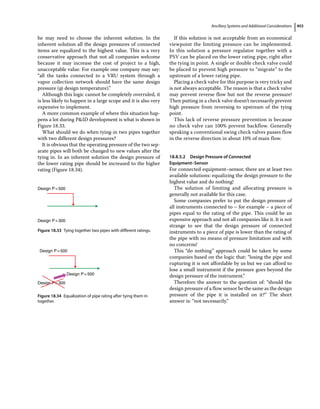
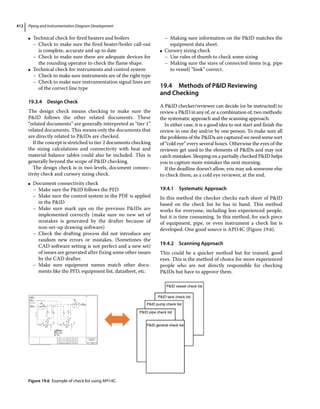
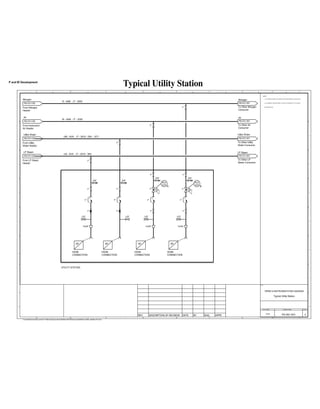
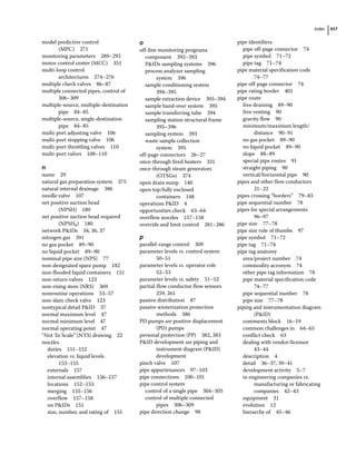
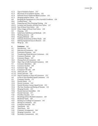
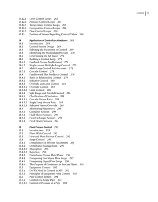
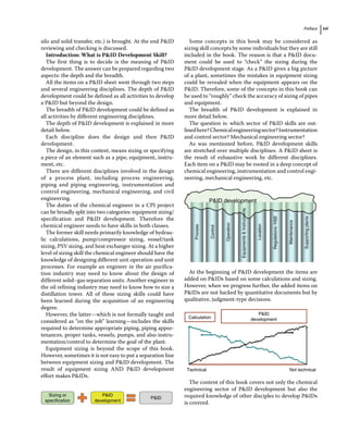
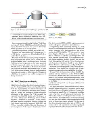
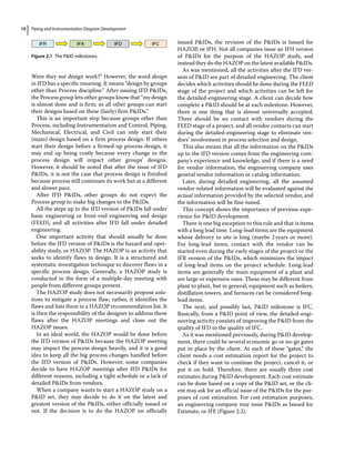
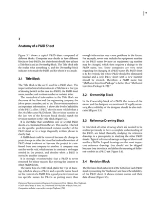
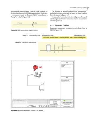
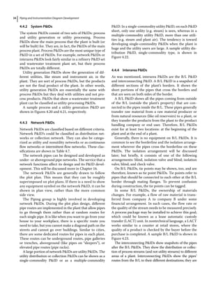
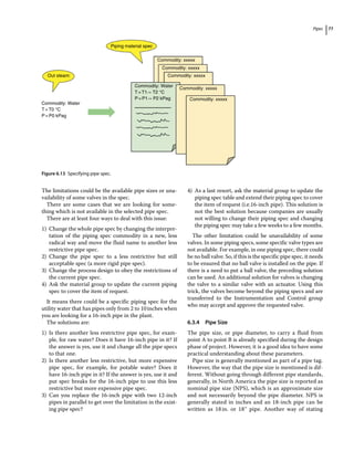
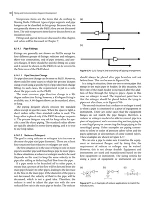
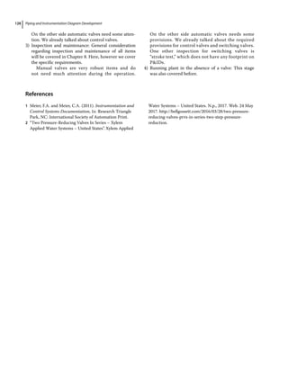
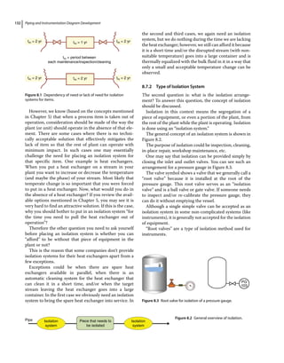
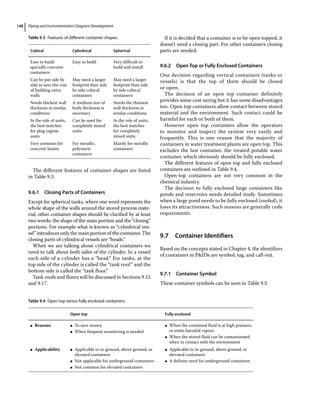
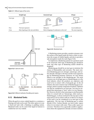
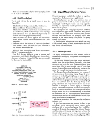
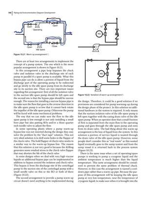
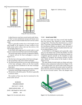
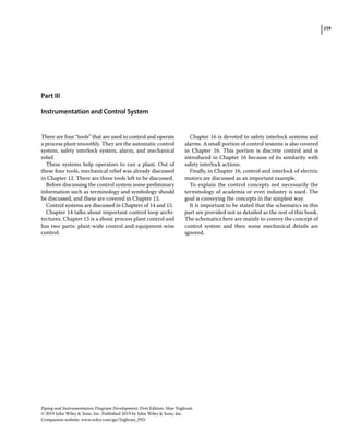
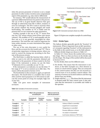
The Revision block basically shows the creation history
of a PID sheet. By studying the Revision block, one can
know when each revision of PID was issued and who
are involved in the PID development and approval. The
different revisions were discussed in Chapter 2.
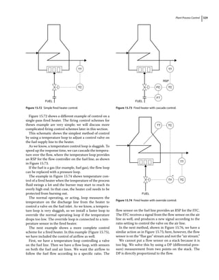
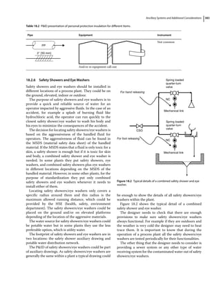
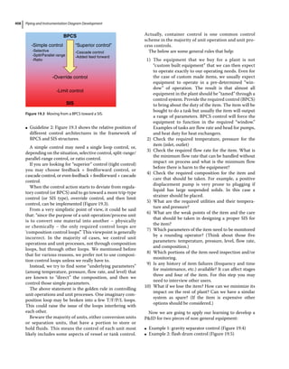
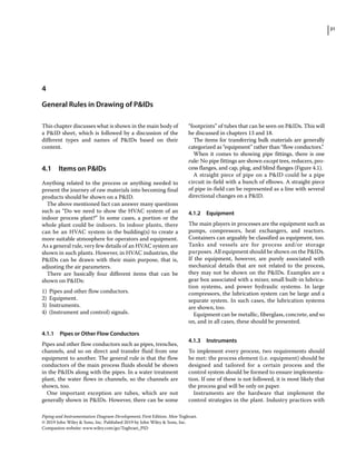
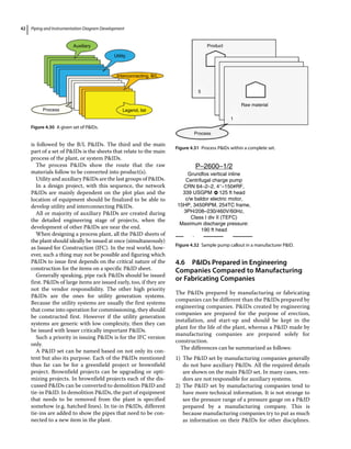
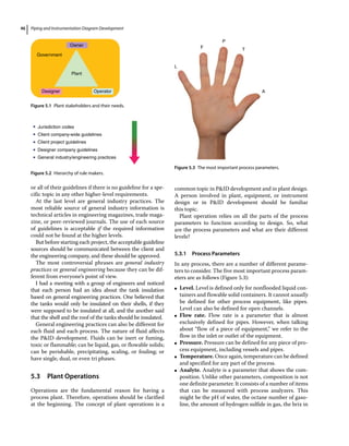
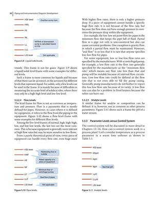
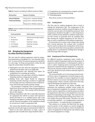
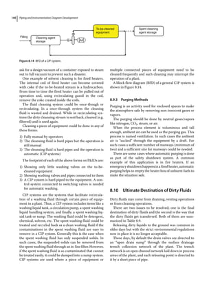
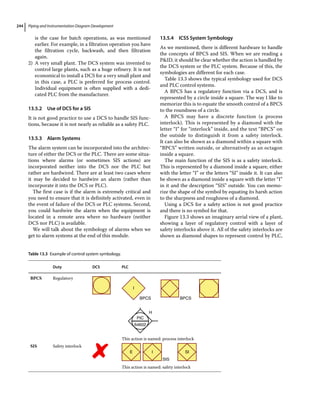
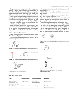
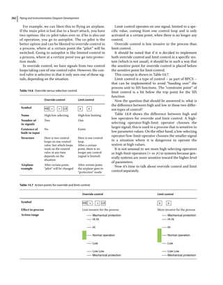
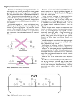
3.5 ­Comments Block
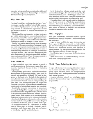
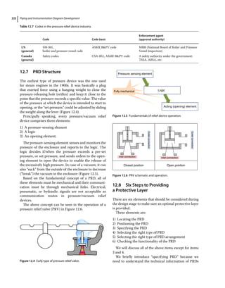
The Comments block is the area where everything that
cannot be pictured in the main body of a PID is shown.
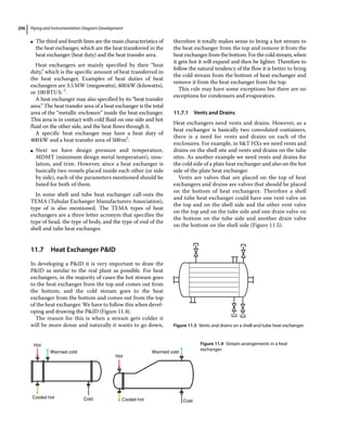
It can have a Holds area and a Notes area (Figure 3.6).
The Holds area is not used by all companies. The
general rule in PID development is that if an item or a
portion of a PID does not meet the quality and com-
pleteness expected for a given revision level, it should be
clouded and the word hold should be written near the
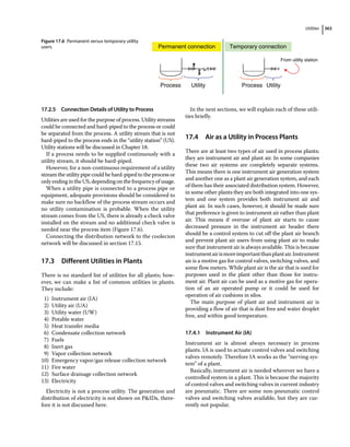
border of the cloud.
Completeness in regard to the revision level of a PID
is very important. If whatever is incomplete is supposed
to be clouded, all the items on the first revision of a PID
(e.g. issue for review [IFR]) should be clouded. But this is
not always the case. In an IFR revision of a PID sheet,
only the items that should be clouded are those that are
expected to be completed and firm in the IFR revision
but are not. Therefore, to be able to decide if one item on
the PID should be clouded, company guidelines should
be followed. In the case of lack of company’s guideline,
Table 19.4 in Chapter 19 can be consulted.
Notes:
Holds:
Reference drawings Revision
block
Company’s logo
Engineering seal
Company registration
Title block
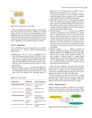
Figure 3.1 The outline of a PID sheet.
Figure 3.2 Typical Title block.
Engineer and permit stamps
This document was prepared exclusively
for XXXX by YYYY and subjects to the
terms and conditions of its contract with
YYYY.......
Legal terms
Permit to practice
Signature:----------
Date:-----------------
Permit number:-------
Figure 3.3 Typical Ownership block.
DWG.No. Reference drawings REV.
A
HVAC detail DWG.
52-27-002
Figure 3.4 Typical Reference block.

37. Anatomy of a PID Sheet 17
For companies that have a Holds area on a PID, the
reasons for the hold can be stated here. The importance
of having a Holds area is that it prevents confusion. For
example, the following conversation highlights this.
The Notes area is where all the information that cannot
be presented as symbols in the main body of a PID are
stated. Because a PID is a visual document and tool, the
Notes should be eliminated or at least the number of
notes should be minimized.
The Notes can be classified in different ways: main
body notes and side notes; specific notes or general
notes; and design notes or operation notes.
Where placing a note on a PID is inevitable, the best
location for a note should be determined, whether in the
main body or the Notes block of the PID. If a note is
specific to an item and is very short, it can be placed on
the main body near the item. But if a note is general or
long, it is better to be placed in a Notes block.
Notes should not be more than three or four words in
the main body of the PID. For a practical approach,
main body notes are more preferable than side notes
because they can be easily recognized compared with
side notes that will be more likely overlooked.
Notes in on the side could be specific or general.
Specific notes are those that refer to specific points of the
PID. Such notes should have the corresponding phrase
“Note X” (X represents the note number in the Notes
block) in the main body of PID. This concept is shown
in Figure 3.7.
One common problem in PIDs are “widowed” notes,
which are the notes in Notes area with no corresponding
phrase in main body of the PID.
General notes refer to any specific area or item on the
PID. These do not have any corresponding Note X in
the main body of PID.
Notes can be classified as design notes or operation
notes depending on their applicability. If a note is placed
for the designers (piping, instrument, etc.) and for the
design duration of a project, it is called a design note. If a
note gives an information to operators or plant managers
during the operation of the plant, it is called an operator
note (Figure 3.8).
Engineer 1: Oh, the pump flanges is still missing? Put the
pump flanges sizes please
Engineer 2: Two month ago I received an email from the
vendor and they said the flange sizes are tentatively 6”
and 4”, but they never confirmed.
Engineer 1: ok, put them here on PID for now.
Later during pump installation it was found that the
flange size by the vendor are not correct and they
wanted to firm it up, which never happened.
This problem could be prevented by putting tentative
flange sizes, cloud it, and in hold area put a comment as:
”To be confirmed by vendor”
0
No. Date Revision
22/10/2010 Issued for approval RP
BY ENG.
LP PE
APPR. APPR.
CL
Figure 3.5 Typical Revision block.
Notes
Holds
1. Vents and drains shall be provided at
the suitable locations during the
construction.
2. Deleted
3. Deleted
4. PVRVs complete with bird screen.
1. The sizes of all relief valves are
preliminary and to be confirmed
during detailed engineering stage.
2. Centrifuge tie-point for vendor
confirmation.
Figure 3.6 Typical Comment block.
Notes:
Note 2
1. XXXXXX
2. Min. suction
length
Figure 3.7 Typical Note in note side area.

38. Piping and Instrumentation Diagram Development
18
Different notes will be discussed in the next chapters
relevant to each process item. Some examples of design
notes and operator notes are shown in Tables 3.1 and 3.2,
respectively.
Sometimes some design notes are not mentioned
because other designers already know what they repre-
sent. For example, the pipe connected to the outlet flange
of pressure safety valve (PSV) should be sloped against
the flow (reverse slope); however, this is not always noted
or mentioned on PIDs because “pipers know this.” In
these cases, no absolute decision can be made. On one
hand, it is impossible to include all the design notes
known to every designer. On the other hand, it is best
not to rely on other designers’ knowledge. Therefore,
the design notes should be put based on the level of
skillfulness of designers involved in the project.
Table 3.1 Typical design notes.
Design note PID symbol Comment
Do not pocket (no pocket) No pocket Prevent creation of gas pocket in intermittent flows, easier
draining when the pipe is out of operation
Min. length Min. length
The suction side of centrifugal pump should be of minimum length
Slug flow Slug flow There is a two‐phase flow in the pipe and its regime is slug flow;
the pipers need to design strong pipe supports to address it
Symmetrical branches Symmetrical
To make sure flow is divided evenly
Locate at ground level Locate at ground level Possibly the pipe is on a pipe rack, but it should be brought down
for the valve
Vertical run Run vertically For safety reasons, the outlet of pressure safety valve; if it releases
to the atmosphere, it should be vertical and upward
FIT should be in the vicinity
of the globe valve (or FIT
should be readable from globe
valve)
Readable from globe valve
FIT
FE
FC For operator during the control valve maintenance: To read the
flow from the flowmeter and adjust the flow by the manual globe
valve accordingly
Full port (FP)
CSO FP
All valves in the route of pressure safety valves should be full port
(or full bore) so as not to obstruct the flow
Table 3.2 Typical operator notes.
Operator note PID symbol Comment
Car seal open
(CSO) CSO FP
All valves in the route
of pressure safety valves
should be CSO to
prevent mistakenly
closed valve
Normally
closed (NC)
NC During the normal
operation of the plant,
this valve should be
closed
Normally no
flow (NNF)
NNF Intermittent stream
Backwash
pipe
Backwash This stream is for
backwashing
Future/spare
nozzle Spare
This nozzle is spare and
for future function
Not important for vendor PKs
PID notes: types
Design notes
Can be added
to
other documents
Should be deleted during
design process
Operation notes
Figure 3.8 Design notes versus operation notes.

39. Anatomy of a PID Sheet 19
Whether to keep the design notes or not is another
issue. Some companies believe that the intention of
design notes is directing other designers during the
design stage of a plant and that all of the design notes
should be eliminated after issuing IFC version of PIDs.
However, other companies leave the design notes
because they can be helpful during the operation of the
plant when something needs to be changed and replaced
with another design note. Also the deletion of each
note – either the design note or the operator note – does
not leave a clean space as the note number should be left
so that the remaining note numbers still stand.
Visual notes can be used in some circumstances. They
can be the detail of construction for a complicated part.
They are, however, are not usually placed on PIDs.
3.6 ­
Main Body of a PID
On the main body of PID, the main elements that can
be seen are “item identifiers,” which will be discussed in
the next chapter.
There is always a debate about what needs to put on
the main body of the PID. If the PID is a focal document
in the process plant, do all the information provided by
all groups need to be put on the PID? It is NOT easy to
decide what and how things should be shown on PIDs;
this topic will be expanded more in Chapter 4.
However, it should be mentioned that the amount of
information shown on a PID can be problematic. Thus
a PID is created “universal” for everyone involved in
process plant.
If the amount of information is not enough, the PID
becomes useless. If the amount of information shown on
PID is too much, the PID also becomes useless because
of its illegibility. It is important to know that a PID will be
used in the process plant during operation, including emer-
gency situations. An operator should be able to grasp the
information needed from a PID as quickly as possible.
However, it is not always easy to gauge and find the
sweet window for the amount of information that should
be shown on a PID (Figure 3.9).
There was a time that there was no single “footprint” of
interlock system on PIDs. Now, a lot of PIDs show the
interlock systems, too.
Lack of information Legibility Congestion
Figure 3.9 The amount of content on PIDs.

40. 21
Piping and Instrumentation Diagram Development, First Edition. Moe Toghraei.
© 2019 John Wiley Sons, Inc. Published 2019 by John Wiley Sons, Inc.
Companion website: www.wiley.com/go/Toghraei_PID
This chapter discusses what is shown in the main body of
a PID sheet, which is followed by a discussion of the
different types and names of PIDs based on their
content.
4.1 ­Items on PIDs
Anything related to the process or anything needed to
present the journey of raw materials into becoming final
products should be shown on a PID.
The above mentioned fact can answer many questions
such as “Do we need to show the HVAC system of an
indoor process plant?” In some cases, a portion or the
whole plant could be indoors. In indoor plants, there
can be an HVAC system in the building(s) to create a
more suitable atmosphere for operators and equipment.
As a general rule, very few details of an HVAC system are
shown in such plants. However, in HVAC industries, the
PIDs can be drawn with their main purpose, that is,
adjusting the air parameters.
There are basically four different items that can be
shown on PIDs:
1) Pipes and other flow conductors.
2) Equipment.
3) Instruments.
4) (Instrument and control) signals.
4.1.1 Pipes or Other Flow Conductors
Pipes and other flow conductors such as pipes, trenches,
channels, and so on direct and transfer fluid from one
equipment to another. The general rule is that the flow
conductors of the main process fluids should be shown
in the PIDs along with the pipes. In a water treatment
plant, the water flows in channels, so the channels are
shown, too.
One important exception are tubes, which are not
generally shown in PIDs. However, there can be some
“footprints” of tubes that can be seen on PIDs. This will
be discussed in chapters 13 and 18.
The items for transferring bulk materials are generally
categorized as “equipment” rather than “flow conductors.”
When it comes to showing pipe fittings, there is one
rule: No pipe fittings are shown except tees, reducers, pro-
cess flanges, and cap, plug, and blind flanges (Figure 4.1).
A straight piece of pipe on a PID could be a pipe
circuit in‐field with a bunch of elbows. A straight piece
of pipe in‐field can be represented as a line with several
directional changes on a PID.
4.1.2 Equipment
The main players in processes are the equipment such as
pumps, compressors, heat exchangers, and reactors.
Containers can arguably be classified as equipment, too.
Tanks and vessels are for process and/or storage
purposes. All equipment should be shown on the PIDs.
If the equipment, however, are purely associated with
mechanical details that are not related to the process,
they may not be shown on the PIDs. Examples are a
gear box associated with a mixer, small built‐in lubrica-
tion systems, and power hydraulic systems. In large
compressors, the lubrication system can be large and a
separate system. In such cases, the lubrication systems
are shown, too.
Equipment can be metallic, fiberglass, concrete, and so
on, and in all cases, these should be presented.
4.1.3 Instruments
To implement every process, two requirements should
be met: the process element (i.e. equipment) should be
designed and tailored for a certain process and the
control system should be formed to ensure implementa-
tion. If one of these is not followed, it is most likely that
the process goal will be only on paper.
Instruments are the hardware that implement the
control strategies in the plant. Industry practices with
4
General Rules in Drawing of PIDs

41. Piping and Instrumentation Diagram Development
22
regard to instruments are not simple and will be dis-
cussed in Chapter 13.
4.1.4 Signals
Signals provide the means for instruments to communi-
cate with each other. After deciding whether an instru-
ment should be shown, the rule for showing signals
would be easy: if there are two separate instruments and
if there is a signal between then, this signal should be
depicted.
Table 4.1 outlines some guidelines on the items gener-
ally shown on the PIDs for each group.
4.2 ­
How to ShowThem: Visual Rules
The first thing that should be answered in regard to the
PID is what goes where and how it is displayed.
The first thing that a reader of a PID expects is leg-
ibility. A PID set is developed by the engineers dur-
ing the design step of the project but will later be used
in a process plant during operations. It is used by indi-
viduals with different levels of knowledge on and
familiarity with a PID. A PID may need to be read
by engineers, managers with management degrees,
trade practitioners, and many others. It also should
give enough information about the project that read-
ers from different backgrounds will be able to under-
stand it. A PID can be used during normal operations
or an emergency event. Therefore, a PID should be
as legible as possible. Below are some rules of thumb
regarding the visual aspects of PIDs:
1) The PID sheet is almost always in landscape orien-
tation (Figure 4.2).
2) Limit the number of main equipment shown on
each sheet. A crowded PID should be avoided.
Some companies try to limit the number of items on
each PID to four or five, but other companies allow
as many as 10.
3) A PID is a pictorial document, so minimize notes
on the PIDs (no “note‐stuffed” drawings).
4) Draw PID symbols as similar as possible to what
an item looks like in reality and approximate to
relative size, but remember, a PID is not drawn to
scale (Figure 4.3).
5) Do not represent the real length of pipes on PIDs.
PID is a “Not To Scale” (NTS) drawing. Therefore,
a short line on a PID could represent a few hun-
dred meters of pipe.
6) Do not “pack” symbols on one side of the PID
sheet. The symbols should be fairly spread out.
7) Generally, an equipment is arranged horizontally on
one level. On an ideal PID sheet, any imaginary
vertical line should, at maximum, cross one equip-
ment symbol. The PID will be too difficult to
understand when equipment symbols are stacked
on each other and the connection between the sym-
bols and the equipment callouts are difficult to be
identified. (Figure 4.4).
8) All the different elements on a PID sheet should be
connected to each other. If a group of elements have
Reducer Tee or O-let
An elbow could be here! Reducer+tee or reduced tee
Figure 4.1 PID representation of pipe circuits.
Table 4.1 Items by different groups on PID.
Group Shown Not Shown
Process Few operational details Process discipline by itself does not have any
element to show.
Mechanical All the equipment in process or “close” to process Mechanical‐related and not Process‐related items
Instrumentation
and Control
Sensors, transmitters, controllers, Automatic valves Signal processing elements, untouchable elements
Piping All pipes, fittings, valves Tubes
Civil Building border, ground border, secondary containment
area, sea‐level concrete equipment
The rest
Electrical Electric motors, electrical heat tracers as symbol The rest

42. General Rules in Drawing of PIDs 23
Figure 4.2 PID orientation.
Figure 4.3 Keeping the relative size of equipment on the PIDs.

43. Piping and Instrumentation Diagram Development
24
no connection to the rest of elements, they can be
drawn on another PID sheet.
9) No visiting stream is allowed. A visiting stream is a
stream that has no connection with other items on
the PID. See Figure 4.5.
10) Do not try to present a PID in a way that follows
geographical directions (e.g. north). PIDs are
drawings independent of these.
The rest of this section outlines the other visual issues
in drawing PIDs and the general practices in dealing
with these issues.
4.2.1 Line Crossing Over
Lines (in different forms) are symbols for pipes or
signals. Crossing lines should be avoided or kept to a
minimum, as well as changing the direction of lines.
However, sometimes both are inevitable,and it is common
to see lines crossing each other in PIDs.
It is important to know that crossing lines in a PID
does not reflect the reality of pipe routes in field. Crossing
lines in the PIDs is not acceptable aesthetically, but it is
Yes
vs.
No
Figure 4.4 Equipment should be fairly distributed horizontally on
the PID.
Figure 4.5 Showing visiting streams is not a good practice.

44. General Rules in Drawing of PIDs 25
unavoidable in some cases. However, pipe crossing (or
better, pipe clashing) in field shows a mistake in the design.
A crossover could be shown in PIDs in two forms, a
“jump” or a “jog” (Figure 4.6).
The decision on which line should be “manipulated”
and which remains intact will be based on the prevailing
line rule shown in Figure 4.7.
For example, in crossing a horizontal process line and
a vertical process line, the horizontal process line remains
intact (Figure 4.8).
4.2.2 Equipment Crossing
Equipment–equipment crossing is not allowed on a
PID (Figure 4.9).
Jump Jog
Figure 4.6 PID representation of pipe crossing.
Most prevailing lines
Horizontal process lines Vertical process lines Instrument signals
Least prevailing lines
Figure 4.7 Lines prevailing rule.
Figure 4.8 Examples of line crossings.
Figure 4.9 Equipment–equipment crossing is not allowed.

45. Piping and Instrumentation Diagram Development
26
Meanwhile, equipment–line crossing can be shown,
but it is not a good practice. This can be managed by
using breaks on the line (Figure 4.10).
4.2.3 Off‐Page Connector
Off‐page connectors are continuation indicators for the
lines, which are pipe and signal symbols. The preference
is to show off‐page connectors horizontally and at the
edge of a PID sheet. The incoming off‐page connectors
are preferably located at the left edge of the PID sheet,
and the outgoing off‐page connectors at the right edge of
the PID sheet.
There are, however, exceptions.
The off‐page connectors in network PIDs (this will
be discussed later in this chapter) can be drawn in vertical
positions, too. This is because network PIDs should
generally follow the plot plans, and sometimes using ver-
tical off‐page connectors prevent crowding on the PID.
In some system PIDs (discussed in section 4.4.2), the
off‐page connectors of utility pipes are shown near the
utility user and not at the edge of the PID sheet. Some
companies adopted this practice to decrease crowding on
the PID by avoiding drawing of long utility lines, which
are not as important as process lines.
The incoming off‐page connectors can be on the right
edge of the PID sheet if they are coming from a down-
stream of the process. The outgoing off‐page connectors
could be on the left edge of the PID sheet if they are
going somewhere on the upstream of the process. The
different appearances of off‐page connectors are shown
in Figure 4.11.
4.2.4 Color in PIDs
Color in PIDs is a recent progress. After the color
printers gained popularity, PID developers decided to
use color PIDs to make them easier and quick to under-
stand. Different colors are mainly used for pipes and sig-
nals because they primarily fill the PID sheets.
4.3 ­
Item Identifiers in PIDs
For each item to be shown on a PID, there can be a
maximum of four different identifiers. This is like indi-
viduals in a society; each individual can be identified by
different identifiers including name, ID number, picture
or symbol, and brief information like eye color, hair color,
height, and so on. Table 4.2 shows this analogy.
Figure 4.10 Equipment–line crossing is allowed.

46. General Rules in Drawing of PIDs 27
Figure 4.12 shows a tank with all four identifiers.
However, neither all items on a PID have all identifi-
ers nor their identifiers are separated from them. For
example, a manual valve may only have symbol and no
other identifier. In the pipe tag, some technical informa-
tion can be seen, too.
To be able to draw a PID, we need to know which
­
identifiers are used for each item and where they can be
found. Table 4.3 shows which identifiers are used by ­telling
which identifier is provided by what group for the PID.
Table 4.4 outlines the identifiers’ location on PID
main body.
4.3.1 Symbols
Symbols are always based on the PID legend sheet,
but the legend sheet is not always the first PID sheet
developed, so it may be difficult for designers to pick a
symbol when there are no legends to refer to. This
issue, however, is not always detrimental. Process engi-
neers generally have some previous experience and
also use symbols that can be understood using com-
mon sense. However, there can be an issue, especially if
Table 4.2 Analogy between a man identifier and a PID
components identifiers.
Analogy: Individual in a
society
Process element on a PID
sheet
Social security no.
Name
Symbol
Age, height,
weight, etc.
Name
Tag
Symbol
Technical information
Figure 4.11 Off‐page connector appearance.
Residual oil tank
T-1200
Residual oil
Dimensions: 10000 mmlD × 15000 mm H
T-1200
Figure 4.12 A single element on the PID.

47. Piping and Instrumentation Diagram Development
28
there are different groups working on different areas
of a project. One group may choose different symbols
for a single element. Therefore, communication plays a
vital role here.
Equipment symbols may have internals that may or may
not be shown. If shown, they should be a dashed line.
4.3.2 Tags
Tags are issued by the group responsible for buying a
given item. Whoever tags an item needs to buy the item.
For example, an equipment tag is issued by the
Mechanical group because they are designated to buy
the equipment for the project. This is similar with piping
tags that are issued by the Piping group.
Tags generally consist of letters and numbers in a
specific arrangement (anatomy). The anatomy of
instrumentation and control (IC) items are mostly
universal and based on International Society of
Automation (ISA) standards. But the tag anatomy for
equipment, pipe, and pipe appurtenances are defined
by the client or project.
For example, in a company, the tag anatomy for equip-
ment could be a representative letter (or block of letters)
and a number, which is a sequence number taken from a
table. When a mechanical engineer wants to tag a tank,
he/she consults with the mechanical procedure docu-
ment to see what the acronym is for a tank. It could be
T or TK. The tank tag will be T‐xx or TK‐xx. The xx here
is a number and the engineer will pick up the number
from their equipment list. Therefore, the tank tag could
be something like T‐231.
The tagging of parallel similar equipment is an inter-
esting issue. One approach is tagging them in a way that
they have the same tag number; the only difference is a
letter at the end of tag number. In this approach, two
parallel similar pumps can be tagged as P‐125A and
P‐125B. Another approach is tagging them like two unre-
lated pumps, such as P‐125 and P‐126. The current trend
is the second approach as the first approach can be
confusing during an emergency and when complete and
clear instructions cannot be heard by the operators. For
example, the instruction “Shut down P‐125A” may be
heard as “Shut down P‐125B” in a noisy environment.
Table 4.3 Source of information for elements’identifiers.
Equipment IC Items Piping Signals
Symbol Per PID legend “Balloons” per PID legend
sheet (possibly based on ISA
legend)
Per PID legend sheet Per PID legend sheet
(possibly based on ISA
legend)a
Tag From equipment list
By Mechanical Engineering
group
From instrument list
(automatic valve list)
By IC group
From the Line List (or LDT)
By Piping group
N/A
Name Process group decision N/A N/A
(unless on off‐page
connectors)
N/A
(unless on off‐page
connectors)
Technical
information
In the form of callout
Decision on components per
project decision, data is
provided by different groups
Per IC group’s decision
(Process group may put
preliminary sizes for control
valves and safety valves)
For pipes, part of their tag,
can be for fittings and their
sizes by Process group
N/A
a
IC, Instrumentation and Control; ISA, International Society of Automation; LDT, Line Designation Table.
Table 4.4 Location of different identifiers for different PID items.
Equipment IC Items Piping Signals
Symbol In the main body of PID
Tag Close to the equipment symbol, but if there is
enough room, inside of the symbol
Inside of
symbol
Close to the symbol N/A
Name Below the tag N/A N/A N/A
Technical
information
Callout: On the top on bottom of main body Close to the
symbol
N/A for pipes, For appurtenances:
close to the symbol
N/A
IC, instrumentation and control.

48. General Rules in Drawing of PIDs 29
4.3.3 Name
Name is something used only for equipment, and generally
the process engineer names the equipment. Some equip-
ment names are assigned in the early stage of a project
when the process flow diagram (PFD) is developed, but
some of the names should be assigned during the PID
development stage.
There is no specific rule for the naming of equipment,
unless it should be unique for each equipment within
each plant to prevent confusion.
The following guidelines are helpful when deciding
about the name for an equipment:
●
● The type of the equipment is part of the equipment and
generally the last word, for example, the word pump in a
boiler feed water pump or the word tank in sales oil tank.
●
● The equipment names are rarely longer than five
words.An acronym can be used if necessary, forexample,
BFW pump rather than boiler feed water pump.
●
● The equipment names are chosen generally based on
their service (e.g. sales oil tank) or their position (e.g.
flotation vessel discharge pump) or both (e.g. disposal
water injection pump).
●
● Where there are several heat exchangers in a series,
the last one (which is likely a utility heat exchanger)
can be named with trim at the beginning.
●
● Where there are two pumps in a series to inject a cer-
tain amount of liquid to the process, the word rough
for upstream pump and trim for the downstream can
be used at the beginning of their names.
●
● Where there are two pumps in a series and the
upstream pump is used to provide enough net positive
suction head (NPSH) for the downstream pump, the
word booster can be used at the beginning of its name
for an upstream pump.
●
● Where a fluid mover takes suction from an important
equipment (like a unit operation or process unit) and
is on the downstream of the equipment, it can be
named as an equipment suction fluid mover like “reac-
tor discharge pump.”
●
● Where a fluid mover feeds an important equipment
(like unit operation or process unit) and is on the
upstream of the equipment, it can be named as an
equipment feed fluid mover like “reactor feed pump.”
4.3.4 Technical Information
Technical information is information about an item on
the PID. The number and nature of information
required to be placed for each item can be decided by the
client. However Table 4.5 can be used in lack of better
information. It is important to consider that the amount
of technical information should be kept at a minimum
on the PIDs. The PID is a pictorial document, and
technical data should only be there to aid in the under-
standing of the symbols. If more numerical information
about an item on a PID is needed, data sheets and other
respective documents need to be consulted.
One general rule that applies to putting the sizes for
pipes, fittings, and valves is that if their sizes can be rec-
ognized from the adjacent items on a PID, there is no
need to show their size. For example, some companies
instruct their PID designers to not put the size of
reducers because it can easily be figured out from the
attachedpipesandtheirtags.ThisisshowninFigure4.13.
Here, we focus only on equipment callouts as they need
more explanations. Equipment callouts detail informa-
tion about a piece of equipment up to roughly less than 10
short lines. Equipment callouts can be introduced in the
general form of a Tag + Name + Additional Data. The
information contained in equipment callouts is collected
from different groups. However, the type of information
required to be placed in callouts can be decided by the
client. Equipment callouts are is shown above each piece
of equipment and on the top edge of the PID sheet.
Some companies use another approach for positioning
the equipment callout on a PID. In this method, the
callouts of static equipment should be placed on the top
of a PID sheet, whereas the callouts of rotary equip-
ment should be placed on the bottom of a PID sheet
(Figure 4.14).
The anatomy of a callout is not arbitrary and is speci-
fied in guidelines by the client or engineering company.
A typical equipment callout may have the structure
shown in Figure 4.15.
Generally speaking, all equipment callout starts with
the equipment tag and equipment name in one line. The
next line of equipment callouts enumerates one to three
mechanical characteristics of the equipment. These
mechanical characteristics should be measurable param-
eters such as the diameter and height for tanks, flow rate
Table 4.5 Type of technical information for different items.
Technical information
Equipment In the form of callout; refer to text for explanation
IC items Sensors: range
Automatic valves: size (and pressure rating)
Pressure safety valve: set point, size (including
inlet and outlet size and orifice designation letter)
Piping Pipes: as part of their tag, pipe size and material
code
Manual valves: size (and pressure rating)
Nozzles: size (and pressure rating)
Fittings: their main sizes
Signals N/A
IC, instrumentation and control.

49. Piping and Instrumentation Diagram Development
30
and head for pumps, or heat transfer area for heat
exchangers. A person with minimum or no knowledge
about the process of the equipment should be able to
measure the parameter(s).
For example, the parameters on a PID for a tank may
be diameter and height or maximum volume (capacity),
but not the normal capacity. For a heat exchanger, the
parameter listed may be the heat transfer area (which
can be measured by estimating all tubes’ peripheral areas
in a shell and tube heat exchanger), but not heat duty,
which is the heat transfer value during the operation.
The next line in the callout box is the sparing policy or
philosophy, which can be explained using the concept of
spare tires for cars. For example, you may have a total of
five tires for a car; four of them are on the car, and one is
a spare in the trunk.
Figure 4.13 The concept of“no repetition”on a sheet of a PID.
Figure 4.14 Positioning of callout for
equipment.

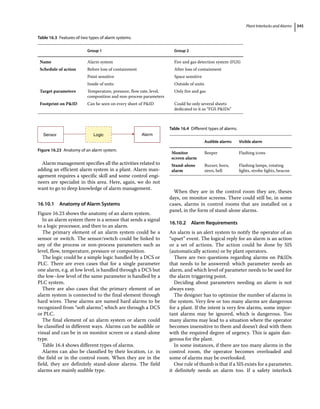
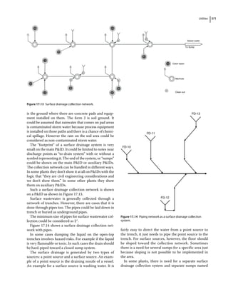
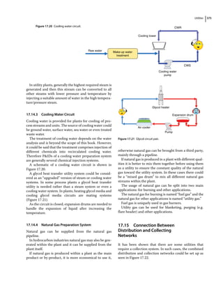
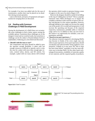
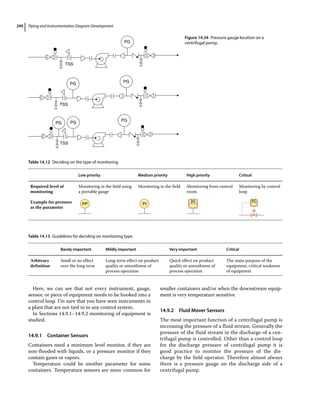
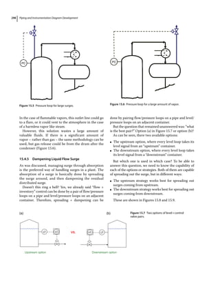
50. General Rules in Drawing of PIDs 31
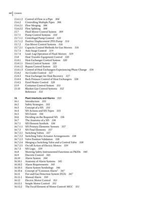
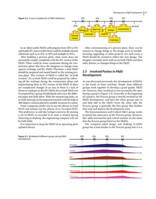
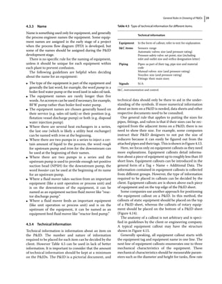
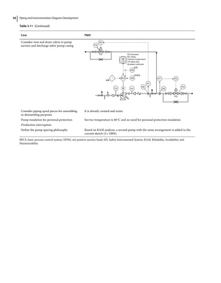
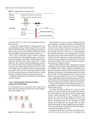
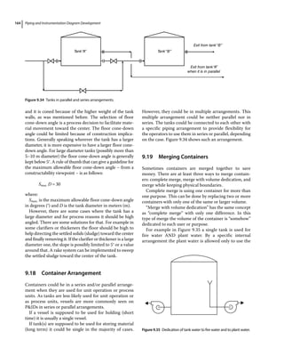
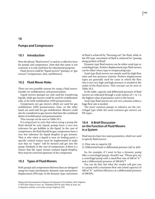
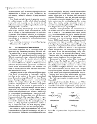
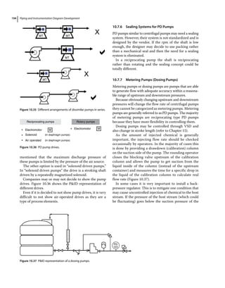
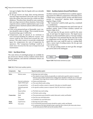
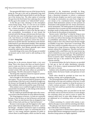
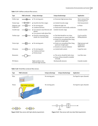
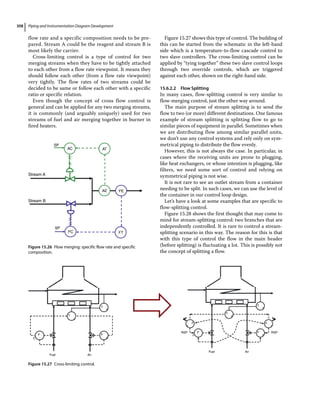
So, the sparing philosophy for tires for the car in this
example is 5×25%; this means four of them are operating
tires and one of them is a spare.
How is 5 × 25% interpreted as four operating ties and
one spare tire?
100
25
4 4 operating tires
5 4 1 1 spare tire
The 100 in the calculation is a fixed number.
In process plants, the sparing philosophy is a parame-
ter that is mainly defined as a need for parallel units. For
single equipment, the sparing philosophy is simply
1×100% and possibly does not need to be mentioned on
the PIDs. The other examples of sparing philosophy is
shown in Table 4.6.
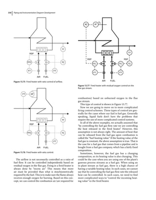
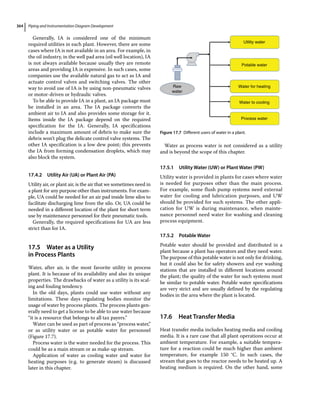
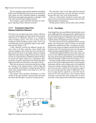
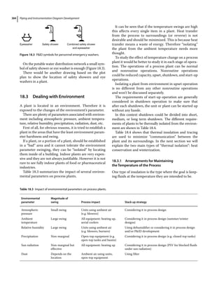
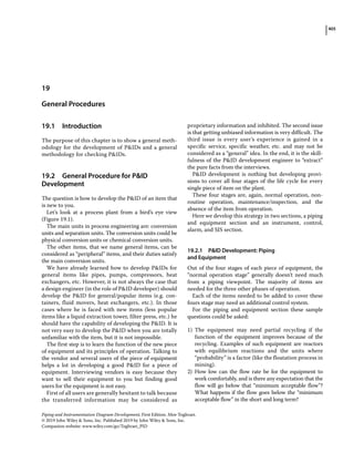
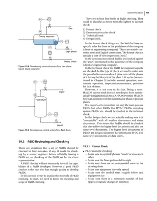
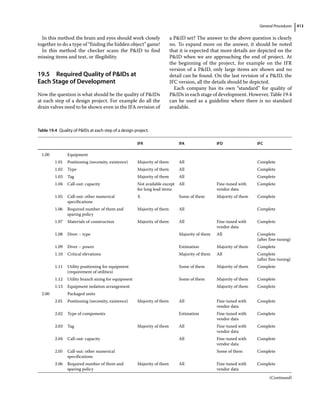
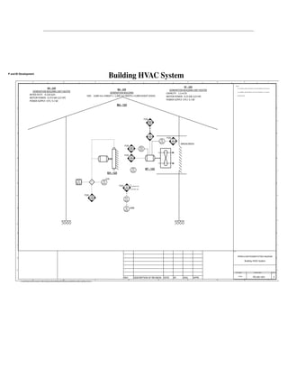
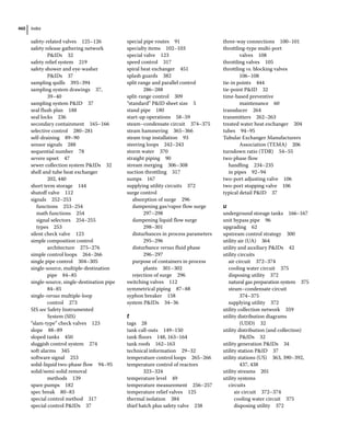
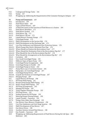
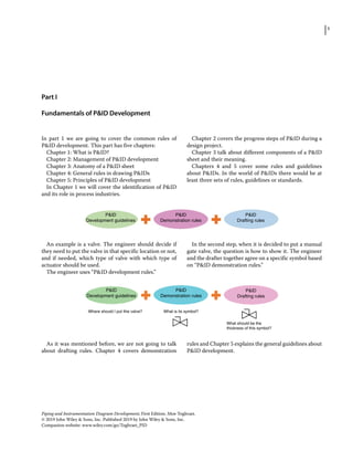
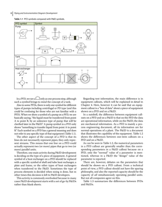
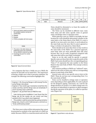
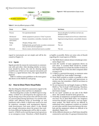
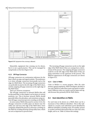
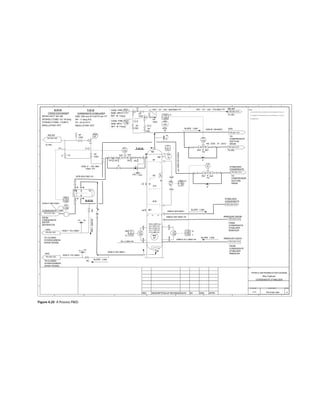
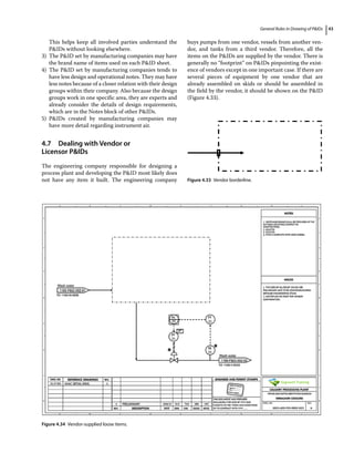
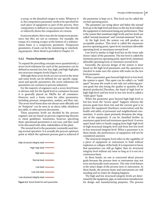
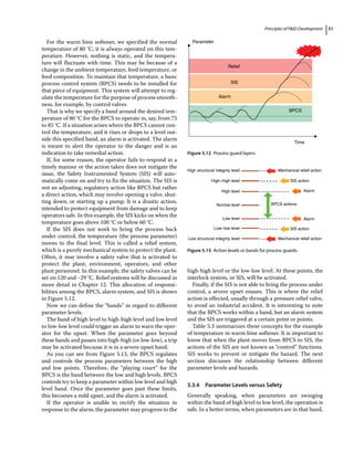
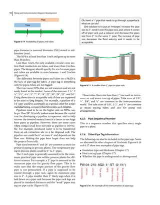
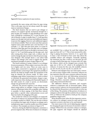
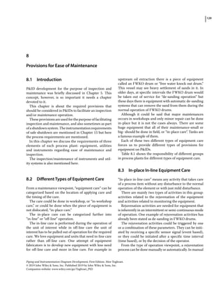
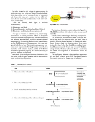
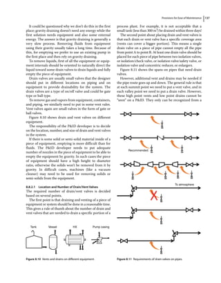
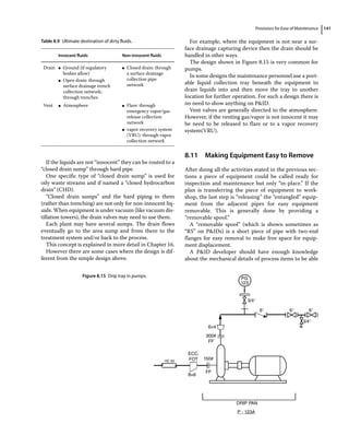
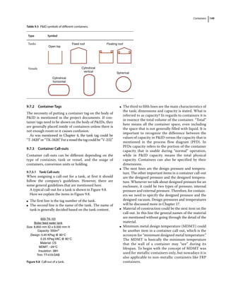
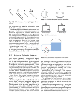
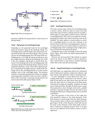
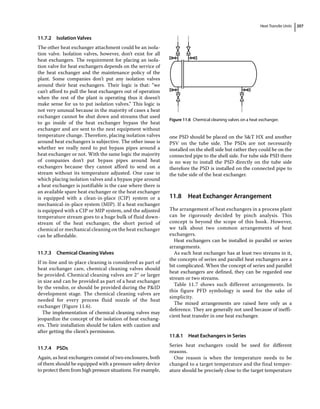
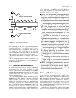
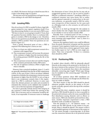
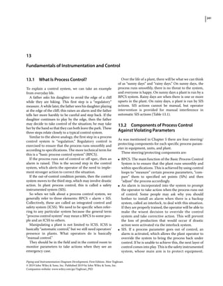
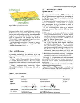
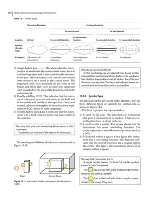
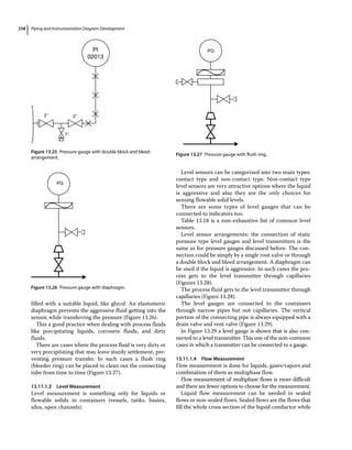
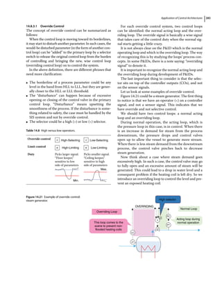
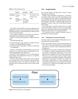
There are some variations of expressing a sparing
philosophy. For example, there can be three sand filters
in parallel that all function during normal operation, but
when one of them is out of service and backwashing is
applied, just two of them are doing the filtration. This
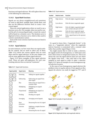
sparing philosophy can be shown in Figure 4.16.
However, when the sparing approach is more compli-
cated, it could be more difficult to show it as a simple
block of a number of parallel equipment multiplied into
a percentage value. More complicated type of sparing
schemes will be discussed in Chapter 5.
Design pressure and design temperature are the next
items in an equipment callout. The design pressure is the
pressure with which the container or a piece of equip-
ment can operate continuously with no safety hazard.
Equipment tag Equipment name
Main equipment parameter(s) [one or two]
Sparing philosophy
Trim no.
Lining/coating/insulation
DP@DT
Figure 4.15 The anatomy of a callout.
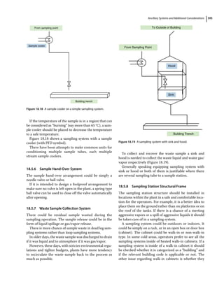
Water from source
Dirty B/W water
Dirty B/W header
Treated water header
To waste management system
From wells
From treated water tank
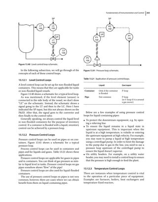
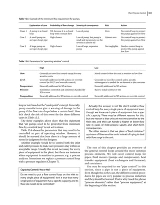
FC
11
SG
12
SG
11
KV
11 21
FY
11
FC
21
SG
22
SG
21
KV
FY
21
FT
11
FE
11
FT
21
FE
21
31
FC
31
SG
32
SG
FL-100A FL-100A FL-100B
31
KV
FY
31
FT
31
FE
31
Filtered water
To treated water tank
Clean B/W water
Feed water header
200-FL-100 A/B
Water sand filter
Capacity: 600 m3/h
Sparing philosophy:
3×33% (normal)
2×50% (backwash)
B/W header
Figure 4.16 Sparing philosophy of three filters during normal operation and only two filtering during backwash.
Table 4.6 Examples of sparing philosophies.
Sparing philosophy notation Sparing philosophy meaning
1×100% 100
100
1 1Operating
1 1 0 No Spare
2×100% 100
100
1 1Operating
2 1 1 1 Spare
3×50% 100
50
2 2 Operating
3 2 1 1 Spare
4×33% 100
33
3 4 Operating
4 3 1 1 Spare
5×25% 100
25
4 4 Operating
5 4 1 1 Spare

51. Piping and Instrumentation Diagram Development
32
Stating the design pressure without talking about the
design ­
temperature is meaningless. Each design pressure
should be stated at a specific design temperature because
generally at higher temperatures, construction materials
lose their strength.
The pair of design pressure and design temperature is
generally defined for containers and the casing of
equipment.
It is important to know that a piece of equipment keeps
its structural integrity up to its design pressure and
design temperature, but it does not necessarily func-
tion properly at the pair of pressure and temperature.
The trim tag can be a confusing term in callouts. “Trim”
in this context means all short pipes are connected to a
piece of equipment. For example, all container nozzles have
a short portion of pipe. A pump has a drain valve and a vent
valve connected to the pump casing through short pieces of
piping. These pipes need tags, and their tags are listed in
the equipment callout. The structure of a trim tag is very
similar to a piping tag. The trim number basically specifies
the construction material for these little pipes connected to
a piece of equipment. It is important to know that the con-
struction material for these short pipes is not necessarily
the same with that of the equipment. We may have more
than one trim number in an equipment callout. These
short pieces of pipes can be inlet or outlet nozzles in con-
tainers, drainage vents in pumps, and other equipment.
It is good to note that equipment and the connecting
pipes were already tagged; the only “missing” tagging
is for the short pipes connected to the equipment
which now is covered by the concept of “trim”.
The last line of a callout can be a brief introduction about
layers around the equipment. The layer can be lining, coat-
ing, or insulation for the equipment. Linings are a protec-
tive layer on the internal surface of a piece of equipment for
protection against the impact of the fluid. Coating is a pro-
tective layer on the external piece of equipment for protec-
tion against the impact of weathering on the external side of
the equipment walls. Insulation is applied for different rea-
sons including heat loss abatement or sound protection.
For example, Figure 4.17 is a callout of a vessel that
contains:
●
● Vessel tag provided by the Mechanical group.
●
● Vessel name provided by the Process group.
●
● Vessel size provided by the Process group and confirmed
by the Mechanical group.
●
● Design temperature and pressure of the vessel provided
by the Process group and confirmed by the Mechanical
group.
●
● Minimum design metal temperature (MDMT) is
requested by Process group and will be provided by the
Mechanical group. (The MDMT will be discussed later.)
●
● Features of the insulation wrapped around the vessel
provided by the Process group (the insulation feature
will be discussed later).
●
● The trim tag provided by the Process group based on
the piping specifications document prepared by the
Piping group. (The trim tag will be discussed later.)
4.4 ­Different Types of PIDs
There are primarily five different types of PIDs: legend
PIDs, system PIDs, network PIDs, interarea PIDs,
and detail PIDs. Although not all companies recognize
the different types of PIDs, the concept exists and
needs to be understood.
The legend PIDs are a few PID sheets that intro-
duce all the symbols and acronyms and their meaning.
To be able to read and understand the PIDs, there
needs be one or more sheets showing the meaning of
symbols and acronyms on the PIDs.
The core of PIDs, system PIDs are the PIDs that
show the material changes.
The network PIDs are the PIDs that show the
distribution or collection of material within the plant
units, for example, utility distribution (and collection)
PIDs, safety release gathering network PIDs, fire
water PIDs, sewer collection system PIDs, and blanket
gas and vapor recovery unit (VRU) PIDs. Some compa-
nies use other names for utility PIDs such as utility
distribution diagrams (UDD) or UIDs. It is easy to
determine if a PID is a network PIDs – these are
mainly pipes and does not have equipment.
Interarea PIDs show where pipes or signals pass from
one area to another area. There are two types of interarea
PIDs: interconnecting PID and battery limit (B/L)
PID. The former shows the passing internal borders of
a plant through different units of the plant, and the latter
shows the passing of the plant border (i.e. plant B/L). The
other name of a B/L PID is “tie‐point PID.”
Equipment tag Equipment name
300 V-4125
Reflux Drum
Size: 4000 ID mm × 5000 mm T/T
Design: 970 kPag @ 70°C/FV @ 120°C
MDMT: –29 °C
Insulation: H/50 mm
Trim: 565NG2167–BAS
Lining: epoxy
Main equipment
parameter
(one or two)
Coating/lining
Trim
Design T and Design P
Figure 4.17 Example of a callout for a vessel.

52. General Rules in Drawing of PIDs 33
Interarea PIDs may have some features of network
PIDs, but the pipes shown on them are straight and do
not have a spider web appearance.
ThelasttypeofPIDsisdetailPIDs.ThesePIDsshow
details of some systems that are not related to the main pro-
cess and do not need to be shown on process PIDs.
The term auxiliary PIDs can be used differently in
each company. Some use it to refer to a detail drawing,
while others use it when referring to the detail PIDs
and legend sheets or even vendor or licensor drawings.
Figure 4.18 summarizes the classifications of PIDs.
4.4.1 Legend PIDs
Generally, the first few sheets of a set of PIDs contain
the list of all PIDs and a legend sheet. Similar to a
table of contents of a book, this list enumerates all the
PIDs in the set with their tags and their descriptions.
The other few sheets are legend sheets where all the
symbols and acronyms used in a set of PIDs are
explained. A sample PID legend sheet is shown in
Figure 4.19.
PIDs
System PIDs Network PIDs Legend PIDs Interarea PIDs Detail PIDs
Process PIDs Utility generation
PIDs
Interconnecting
PIDs
Tie-in PIDs
Figure 4.18 PID type classification.
NOTES:
TITLE
PIPING INSTRUMENTATION DIAGRAM
####### BB
CHK
AA
APPR
APPROVED FOR DESIGN
0
H I
8
A B C D E F G H
0
03-C-3598
8300-25I-001- A
I
6
7
8
BY
REV DESCRIPTION OF REVISION DATE
LEGEND SYMBOLS
Mohammad Toghraei
CC
1
2
3
4
7
2
3
4
5 5
6
1
A B C D E F G
PROJ NUMBER DRAWING NUMBER REV NO
Line
designations
Line
commodities
Pipe finishing Misc. symbols Abbreviations Notes
M
W = Water
PP = Personal
protection
VB = Vortex
Breaker
Typical instrument identification
Line symbols Instrument
signal
symbols
Instrument
symbols
Equipment
symbols
Valve,
control valve,
safety valve
symbols
Sensor
symbols
Figure 4.19 A PID legend sheet.

53. Piping and Instrumentation Diagram Development
34
4.4.2 System PIDs
The system PIDs consist of two sets of PIDs: process
and utility generation or utility processing. Process
PIDs show the main process that the plant is built (or
will be built) for. They are, in fact, the PIDs of the main
process plant. Process PIDs are the most unique type of
PID in a set of PIDs. For example, network PIDs or
interarea PIDs look fairly similar in a refinery PID set
and wastewater treatment plant set, but their process
PIDs are totally different.
Utility generation PIDs show the generation of dif-
ferent utilities, like steam and instrument air, in the
plant. They are sort of process PIDs, but the products
are not the final product of the plant. In other words,
utility generation PIDs are essentially the same with
process PIDs but they deal with utilities and not pro-
cess products. PIDs that show a wastewater treatment
plant can be classified as utility‐processing PIDs.
A sample process and a utility generation PID are
shown in Figures 4.20 and 4.21, respectively.
4.4.3 Network PIDs
Network PIDs are classified based on different criteria.
Network PID’s could be classified as distribution net-
works or collection network. They can also be catego-
rized as utility and nonutility networks or as continuous
flow networks or intermittent flow networks. These clas-
sifications are shown in Table 4.7.
The network pipes can be designed and developed as
under‐ or aboveground pipe networks. The service that a
network functions affect its design and its PID devel-
opment. This will be discussed more in Chapter 16.
The network PIDs are generally drawn to follow
the plot plan. This means that they can be roughly
superimposed on plot plans. If there is a need to show
any equipment symbol on the network PID, it can be
shown in plan view, rather than the more common
side view.
The Piping group is highly involved in developing
network PIDs. During the plot plan design, different
pipe routes are implemented in the plant that allow pipes
to go through them rather than at random routes for
each single pipe. It is like when you want to go from your
house to your workplace, there is a specific route you
need to take, but you cannot make a diagonal path on the
streets and cannot go over buildings. Similar to cities,
there are some dedicated routes for pipes in each plant.
These routes can be underground routes, pipe galleries
or trenches, aboveground (like pipes on “sleepers”), or
elevated pipe routes (pipe racks).
A large portion of network PIDs are utility PIDs. The
utility distribution or collection PIDs can be shown as a
single‐commodity PID or as a multiple‐commodity
PID. In a single‐commodity utility PID, on each PID
sheet, only one utility (e.g. steam) is seen, whereas in a
multiple‐commodity utility PID, more than one utili-
ties (e.g. steam and plant air). The tendency is toward
developing single‐commodity PIDs when the plant is
huge and the utility users are large. A sample utility dis-
tribution PID, single‐commodity type, is shown in
Figure 4.22.
4.4.4 Interarea PIDs
As was mentioned, interarea PIDs are the B/L PID
and interconnecting PID. A B/L PID is a snapshot of
different sections of the plant’s borders. It shows the
short portions of the pipes that cross the borders and
that are seen on both sides of the border.
A B/L PID shows all the pipes coming from outside
of the B/L (outside the plant’s property) that are con-
nected to the pipes inside the B/L. These pipes generally
transfer raw material from a raw material producer or
from natural resources (like oil reservoirs) to a plant, or
they transfer the products from the plant to the product
handling company or end user. Therefore, B/L PIDs
exist for at least two locations: at the beginning of the
plant and at the end of a plant.
Generally, there is no equipment on B/L PIDs. It is
common to see the borderline and the isolation arrange-
ment wherever the pipes cross the borderline on these
PIDs. The isolation arrangement will be discussed
later; but briefly, it consists of one of the following
arrangements: blind, isolation valve and blind; isolation
valve, blind, and check valve.
On B/L PIDs, tie points may be shown, too, and are
therefore, known as tie point PIDs. Tie points refer to
pipes that should be connected to each other at the B/L
border through mating flanges. To prevent confusion
during construction, the tie points can be tagged.
In some B/L PIDs, the ownership of materials
changes. For example, a flow of raw material is trans-
ferred from company A to company B under some
financial arrangement. In such cases, the flow rate or
the quality of the stream needs to be measured precisely.
A process package may be installed to achieve this goal;
which could be known as a lease automatic custody
transfer (LACT) unit. In nontechnical language, a LACT
works similar to a counter at retail stores, where the
quality of a product is checked by the buyer before the
purchase is completed. A sample B/L PID is shown in
Figure 4.23.
The interconnecting PIDs show snapshots of the pipes
after the B/L PIDs. They show the distribution or collec-
tion of process streams (and not utility streams) to different
areas of a plant. Interconnecting PIDs show the pipes’
routes from the B/L to their different destinations; they are

54. REV DESCRIPTION OF REVISION DATE BY ENG. APPR.
PIPING INSTRUMENTATION DIAGRAM
Moe Toghraei
CONDENSATE STABILIZER
PD-0120-1001 0
HS - DVA - 6 - 2012 -
HCB-4-025-CN21-
CASE: FIRE
SIZE: 6R10
SET: @ 11barg
PID-0120-1001
CONDENSATE
FROM
CONDENSATE
WATER
SEPARATOR
To HFL
E-3112
CROSS EXCHANGER
RATED DUTY 361 kW
DP(SHELL/TUBE): 23 / 30 barg
DT(SHELL/TUBE): 175/80°C
INSULLATION: HOT
LIT
124
MW
24
HHLL=5870 mm
HLL=4870 mm
NLL=3,050 mm
LLL=1,450 mm
LLLL=305 mm
8
M1
N
N2
T-3112
LIT
123
4
6x4 6x4
4
FC
EL=1,500 mm
PY
123
T
15
15
TIT
GAS
TO
COMPRESSOR
SUCTION
DRUM
PID-020-1010
IS
OS
HH LI
124
LL
2
8
7
S
S
T1
T
FP
CSO
LC
2
PID-030-1001
HCB- 2 - 120 -983-
CN01 -PT
FP
CSO
4
6x4 6x4
4
FC
PID-020-1010
PID-020-1010
123
PIT
PIC
123
LY
12
LIC
123
H
FIT
123
FIC
123
123
PD
IT
4x3 4x3
3/4
3/4
3/4 3/4
4
B2
4
CN21
PID-0120-1010
PID-0120-1010
PID-0120-1010
PD
15
H
FP
CSO
PID-020-1010
To HFL
FP
CSC
FP
CSO
FP
CSO
HFL - 12 - 120 - 779-AN21-PT
PSV
11A
CASE: FIRE
SIZE: 6R10
SET: @ 11barg
PSV
11B
HFL - 12 - 120 - 559-AN21-PT
M
24
24
AN21
PSV
12
To HFL
FROM
CONDENSATE
STABLIZER
REBOILER
FROM
CONDENSATE
STABLIZER
REBOILER
HCD
AG
UG
T-3112
CONDENSATE STABILAZER
SIZE 1200 mm ID X18770 mm T/T
DP : 11 barg (FV)
DT: -23.5/175°C
INSULLATION: HOT
PY
123
E-3112
HCB-203-CN21-IH
GAS-8-156-AN21-
TO
COMPRESSOR
SUCTION
DRUM
STABILIZED
CONDENSATE
REBOILER VAPOR
REBOILER LIQUID
SLOPE
1:200
HCB-3''
-
227-AN01-PT
HSB-8-204-AN21-
HSB-8-207-AN21-IH
HSB-3-211-AN21-IH
SLOPE 1:200
SLOPE 1:200
SLOPE 1:200
H
L
N3
#2
#3
#15
#18
RELIEF
STABILIZED
CONDENSATE
RELIEF
TO CLOSED
HYDROCARBON
DRAIN VESSEL
TO CLOSED
HYDROCARBON
DRAIN VESSEL
AG
PID-030-1001
HCD
PID-030-1001
NC
NC
HCB-3''-207-AN01-
HCB-3''-101-AN01-
HCB-1''-701-AN01-
SLOPE 1:200
Figure 4.20 A Process PID.

55. Piping and Instrumentation Diagram Development
36
also based on the plot plan of the plant. A typical intercon-
necting PID sheet is shown in Figure 4.24.
4.4.5 Detail PIDs
The last part of a set of PIDs is the detail PIDs.
When some items are removed from the main PIDs
for the sake of legibility and put on other PIDs, those
are the detail PIDs. Therefore, each sheet of the detail
PID should be referred from one or more main
PIDs.
The systems shown on detail PIDs comprise
­
systems that have any of the following features or a
combination:
Table 4.7 Different services of network PIDs.
Distribution or
collection network
Utility or nonutility
network
Continuous flow or
intermittent flow
Utility distribution PIDs Distribution Utility Continuous flow or
intermittent flow
Utility collection PIDs Collection Utility Continuous flow or
intermittent flow
Relief and blowdown PIDs Collection Nonutility Intermittent flow
Fire water distribution PIDs Distribution Can be considered as
utility or nonutility
Intermittent flow
Sewer collection system PIDs Collection Utility Intermittent flow
Blanket gas distribution PIDs Distribution Utility Intermittent flow but very
frequent
Vapor recovery unit PIDs Collection Utility Intermittent flow but very
frequent
Figure 4.21 A Utility Generation PID.

56. General Rules in Drawing of PIDs 37
●
● Systems that are not directly related to the main pro-
cess of a plant.
●
● Systems whose deletion from the main PIDs does not
hinder the understanding of the process (also cuts
down on the crowded look) and eases readability.
●
● Systems that appear on several PID sheets and are
exactly the same.
If a detail PID is referred to by several main PIDs,
the detail PID is named “typical detail PID”, but if a
detail PID is referred to by one main PID, the detail
PID is named “nontypical detail PID”. Examples of
typical detail PIDs are pump seal flush, sampling sys-
tem PID, safety shower and eye‐washer PIDs, utility
station PID, special control PIDs (remotely operated
valves, electric motors), piping detail PID, and HVAC
equipment PIDs. Examples of nontypical detail PIDs
are rotary machine lubrication and fire or gas detection
and deluge system.
A referred detail of a PID can be written down near
the system in the main PID, or the detail PID can
simply be mentioned as one of several “reference” PIDs
on the main PID.
Some companies show the content of detail PIDs in
the guidelines and not on a PID. For example, a com-
pany may not like developing special control PIDs and
display relevant information in the IC design guide-
lines. Piping detail PIDs, which may have hook‐up
piping detail of sensors, steam traps, and instrument air
manifolds, may not be provided in a PID and instead
be mentioned in the Piping design guidelines.
Some of the types of detail PIDs are explained below.
●
● HVAC drawings: These represent the HVAC system
for industrial buildings. A sample HVAC PID is
shown in Figure 4.25.
●
● Sampling system drawings: Sometimes the plant has
many different sampling systems for the sampling of
REV DESCRIPTION OF REVISION DATE BY ENG. APPR.
HOT WATER DISTRIBUTION
0
PD-300-1003
From wash water
recycle pump
Wash water
To XXXX
Wash water
WAT - AA - 8″ - 3018
WAT - AA - 4″ - 3019
Wash water
To XXXX
WAT - AA - 6″ - 3020
Wash water
To XXXX
WAT - AA - 4″ - 3021
Wash water
To XXXX
WAT - AA - 2″ - 3022
Wash water
To XXXX
WAT - AA - 2″ - 3023
Intermittent
Figure 4.22 A Utility Distribution PID.

57. Edward’s pipeline company John’s plant company
Figure 4.23 A Battery Limit PID.
Figure 4.24 A Utility Distribution PID.

58. General Rules in Drawing of PIDs 39
gases, liquids, or even flowable solids. If this is the
case, it may be all of the details of the sampling system
are not shown on the main PIDs and instead col-
lected together and put at the end of the PID set; so
what is seen on the main PIDs may be only a “bal-
loon” representing a typical sampling system. A sam-
ple PID sheet with a reference to a sampling system
PID is shown in Figure 4.26, along with the sampling
system PID (Figure 4.27).
●
● Pump seal flush drawings: A shaft generally penetrates
a casing while it rotates. Examples of this are shafts for
pumps, compressors, and mixers. The opening for the
shaft should be loose enough to allow the shaft to
rotate and tight enough to prevent any type of leaking.
This problem is effectively solved by a mechanical seal.
Mechanical seals are devices made up of two blocks of
graphite sliding over each other. One block, which is
shaped like a doughnut, is connected to the shaft, and
the other block, in the form of a disk, is connected to
the casing.
A mechanical seal needs to have a system for lubricat-
ing, flushing, and cooling. Such a system is called a seal
flush system.
Sometimes companies decide not to show all the
details of mechanical seals on the main PID to reduce
crowding and because these items are not related to the
main process of plant. In this case, the specific seal flush
system used for a specific pump is mentioned on the
main PID, and the reader is referred to the appropriate
seal flush plan PID for the details. A sample PID sheet
with a reference to a seal flush system sheet is shown in
Figure 4.28, along with the seal flush PID in Figure 4.29.
4.5 ­
A Set of PIDs
A set of PIDs may consist of different types of PID
sheets. Figure 4.30 shows a typical order in a set of PIDs.
The legend PIDs are logically the first PIDs because
they list the meaning of the symbols and acronyms. This
Supply fan
Air handling unit
Cooling coil Heating coil Filter
Figure 4.25 An HVAC PID.

59. Piping and Instrumentation Diagram Development
40
PID-300-1003
Wash water
To wash water pre-h
- 8″ - 3015
B C D E F G
Refer to the PID for the type 1
sampling system
4×3 4×3
FO
FC
IS OS
FC
130
FV
130
LV
131
LC
131
WAT - AA - 4″ - 3014
S1
WAT
-
AA
-
4″
-
3017
WAT
-
AA
-
6″
-
3018
WAT
-
AA
-
6″
-
3016
3/4″ 3/4″
2″
6×4
6×4
3″
1″
1″
1″ 1″
1″ 1″
Figure 4.26 A PID sheet with a reference to a sampling system sheet.
SAMPLING SYSTEMS
8300-25I-001- A
Mohammad Toghraei
0
Sampling type Open
Sample Fluidity Complete fluidity
Sample health No issue
Sample Phase Liquid-Low volatility
Sample Temp. 60°C
Sampling Source
Min.
Min.
Sampling Source
Min.
Min.
CMS
3/4
1/2
3/4
1/2
CMR
Sampling Source
Min.
Min.
CMS
3/4
1/2
CMR
Sampling type Open
Sample Fluidity Complete fluidity
Sample health No issue
Sample Temp. 60°C
Sample Phase Liquid-Low volatility
Sample Phase Liquid-Low volatility
Sample Temp. 60°C
Sample Fluidity Highly Viscose
Sample health No issue
Sampling type Open
Utility Steam
Sampling Source
Min.
To Safe location
3/4
1/2
Sampling type Closed Loop
Sample Fluidity Complete fluidity
Sample health No issue
Sample Phase Gas
Sample Temp. 60°C
Sampling System-Type 1 Sampling System-Type 2
Sampling System-Type 4
Sampling System-Type 3
Figure 4.27 A sampling system PID.

60. General Rules in Drawing of PIDs 41
WAT
-
AA
-
6″
-
3018
1″
1″
1″
″
3″
3/4″
FE
140
PG
140
6×4
8×6
M
300-P-130
TSS
PG
141
Seal flush plan 21
This pump uses seal flush system plan
21. Refer to the PID for seal flush
system plan 21 for details
Figure 4.28 A PID referring to a hypothetical seal
flush PID.
API plan 21
M
AC-327
Figure 4.29 A Seal Flush PID.

61. Piping and Instrumentation Diagram Development
42
is followed by the B/L PIDs. The third and the main
part of a set of PIDs is the sheets that relate to the main
process of the plant, or system PIDs.
The process PIDs show the route that the raw
materials follow to be converted into product(s).
Utility and auxiliary PIDs are the last groups of PIDs.
In a design project, with this sequence, the network
PIDs are mainly dependent on the plot plan and the
location of equipment should be finalized to be able to
develop utility and interconnecting PIDs.
All or majority of auxiliary PIDs are created during
the detailed engineering stage of projects, when the
development of other PIDs are near the end.
When designing a process plant, all the PID sheets of
the plant should ideally be issued at once (simultaneously)
as Issued for Construction (IFC). In the real world, how-
ever, such a thing may not be possible and figuring which
PIDs to issue first depends on the critical nature of the
construction for the items on a specific PID sheet.
Generally speaking, pipe rack PIDs should be issued
first. PIDs of large items are issued early, too, if they are
not the vendor responsibility. The other high priority
PIDs are the ones for utility generation systems.
Because the utility systems are usually the first systems
that come into operation for commissioning, they should
be constructed first. However if the utility generation
systems are generic with low complexity, then they can
be issued with lesser critically important PIDs.
Such a priority in issuing PIDs is for the IFC version
only.
A PID set can be named based on not only its con-
tent but also its purpose. Each of the PIDs mentioned
thus far can be for a greenfield project or brownfield
project. Brownfield projects can be upgrading or opti-
mizing projects. In brownfield projects each of the dis-
cussed PIDs can be converted to demolition PID and
tie‐in PID. In demolition PIDs, the part of equipment
that needs to be removed from the plant is specified
somehow (e.g. hatched lines). In tie‐in PIDs, different
tie‐ins are added to show the pipes that need to be con-
nected to a new item in the plant.
4.6 ­
PIDs Prepared in Engineering
Companies Compared to Manufacturing
or Fabricating Companies
The PIDs prepared by manufacturing or fabricating
companies can be different than the PIDs prepared by
engineering companies. PIDs created by engineering
companies are prepared for the purpose of erection,
installation, and start‐up and should be kept in the
plant for the life of the plant, whereas a PID made by
manufacturing companies are prepared solely for
construction.
The differences can be summarized as follows:
1) The PID set by manufacturing companies generally
do not have auxiliary PIDs. All the required details
are shown on the main PID set. In many cases, ven-
dors are not responsible for auxiliary systems.
2) The PID set by manufacturing companies tend to
have more technical information. It is not strange to
see the pressure range of a pressure gauge on a PID
prepared by a manufacturing company. This is
because manufacturing companies try to put as much
as information on their PIDs for other disciplines.
Auxiliary
Utility
Interconnecting, B/L
Process Legend, list
Figure 4.30 A given set of PIDs.
Product
Raw material
Process
5
1
Figure 4.31 Process PIDs within a complete set.
P–2600–1/2
Grundfos vertical inline
Centrifugal charge pump
CRN 64–2–2, 4″–150#RF,
339 USGPM 125 ft head
c/w baldor electric motor,
15HP, 3450RPM, 254TC frame,
3PH/208–230/460V/60Hz,
Class I div II (TEFC)
Maximum discharge pressure:
190 ft head
O
Figure 4.32 Sample pump callout in a manufacturer PID.

62. General Rules in Drawing of PIDs 43
This helps keep all involved parties understand the
PIDs without looking elsewhere.
3) The PID set by manufacturing companies may have
the brand name of items used on each PID sheet.
4) The PID set by manufacturing companies tends to
have less design and operational notes. They may have
less notes because of a closer relation with their design
groups within their company. Also because the design
groups work in one specific area, they are experts and
already consider the details of design requirements,
which are in the Notes block of other PIDs.
5) PIDs created by manufacturing companies may
have more detail regarding instrument air.
4.7 ­
Dealing with Vendor or
Licensor PIDs
The engineering company responsible for designing a
process plant and developing the PID most likely does
not have any item it built. The engineering company
buys pumps from one vendor, vessels from another ven-
dor, and tanks from a third vendor. Therefore, all the
items on the PIDs are supplied by the vendor. There is
generally no “footprint” on PIDs pinpointing the exist-
ence of vendors except in one important case. If there are
several pieces of equipment by one vendor that are
already assembled on skids or should be assembled in
the field by the vendor, it should be shown on the PID
(Figure 4.33).
Figure 4.33 Vendor borderline.
Figure 4.34 Vendor‐supplied loose items.

63. Piping and Instrumentation Diagram Development
44
A licensor can be defined as a specific type of ven-
dor who registered his or her system as intellectual
property and not all of the design can be disclosed to
others, including clients and engineering companies.
Vendor‐supplied systems in PIDs are generally
shown using a dash‐dot border around the system.
All the connecting pipes (but not necessarily tubes)
should show some sort of break (like a flange) at the
vendor border line. This concept will be discussed in
more detail in Chapter 6.
If there are items that should be provided by the
vendor but cannot be surrounded by the vendor border,
a predetermined sign (mentioned in the legend PID)
can show vendor responsibility for those items. The sign
could be a simple star, or letter F (represents “furnished
by vendor”). Figure 4.34 shows this concept.
These vendor‐supplied items, which are outside of
vendor border, generally are transported to the field as
loose items. Engineering companies are not generally
responsible for vendors’ or licensors’ designs, unless
otherwise stated in the contract. Although the con-
cept of showing vendor‐ or licensor‐supplied items is
clear, how companies incorporate these items on to
the PIDs vary.
The vendor PIDs are sometimes implemented into
the master PIDs by redrawing them or “transplanting
the snapshot” of their drawing (Figure 4.34). In other
cases, the vendor border block remains as a blank block
with only a reference sentence to the vendor PIDs
(Figure 4.36).
In all of these examples, except redrawing vendor
PIDs, it should be ensured that the vendor uses the
approved symbols mentioned in the legend PID to
avoid any confusion.
Vendor
Dwg.
Our
Dwg.
Figure 4.35 Integrating vendor PIDs by implementing vendor PIDs into master PIDs.
Figure 4.36 Integrating vendor PIDs by referencing.

64. 45
Piping and Instrumentation Diagram Development, First Edition. Moe Toghraei.
© 2019 John Wiley Sons, Inc. Published 2019 by John Wiley Sons, Inc.
Companion website: www.wiley.com/go/Toghraei_PID
This chapter attempts to answer the important question:
whose benefit, and to what extent, should be considered
in developing PIDs? There is no universal set of rules
for developing PIDs. However, it can be said that
the PID development rules come from the plant
stakeholders.
5.1 ­Plant Stakeholders
The main goal of a plant is producing a product in the
quantity and with the quality expected and designed for.
However, there is more than that. A good plant design
should first consider health, safety, and environmental
codes and standards. The owner’s wishes for the plant
should also be noted, followed by the designer’s and
operator’s requirements (Figure 5.1).
Jurisdictional health, safety, and environmental codes
and regulations cannot be compromised. These rules
are established to guarantee the safety and health of the
society and protect the environment. It is important to
realize the government regulations and codes are the
“minimum” requirements, and some companies decide
to go further to show they are good “corporate citizens”.
For example, the concept of sustainability is not
always – and in its holistic approach – considered in gov-
ernment codes.
The owners of a plant, from an abstract point of view,
are looking for a plant with the minimum required capi-
tal cost and the minimum expending/operating cost.
They also want to have a plant that can be quickly built.
Designers like to work on projects in which the design
bases are well established to make sure their design fits
the purpose of the plant. If the design methods are unre-
liable, designers have two options. They may ask the cli-
ent to do more research, tests, and piloting before
starting a commercial plant, or designers can be asked to
design in a way that addresses the different situations
that may occur.
The operators are the firsthand end users of a plant and
prefer one that can be easily operated and with reasona-
ble flexibility and the highest level of safety. They may not
always think about the capital costs or operating costs,
but sometimes their instructions override the instruction
of others, such as clients, ­
engineers, and managers.
5.2 ­
The Hierarchy of PID
Development Rules
Each of the aforementioned parties initiates its require-
ments through different documents. Codes, regulations,
guidelines, and standards are some of them. When
two or more requirements exist, the designer (PID
­
developer) should select one requirement based on the
hierarchy of the rule makers shown in Figure 5.2.
Rule sets at the highest level are the ones set by
­
jurisdictional bodies. These should be followed with
no exceptions and are generally referred to as codes or regu-
lations that cannot be overturned by any other rule maker.
Next are client guidelines, which may be applicable
within the company or specific to a project. This is the
highest level of rules that the designer should follow. The
client rules sometimes can be waived if a proper “request
for deviation” with adequate supporting documentations
are submitted to the client and the client approves it.
The client may show less resistance to deviation if
there is only company‐wide (and not project‐specific)
guidelines.
Some clients are just small companies, which don’t
have much experience about the plant they want to build.
Then there is no client guideline (neither project-wide
nor company-wide) are available. In those cases, the
designer refers to their own guidelines or the fourth level
of rules or engineering company guidelines.
On the fourth level are the engineering company
guidelines. Large engineering companies may have their
own set of guidelines. They may get approval to use some
5
Principles of PID Development

65. Piping and Instrumentation Diagram Development
46
or all of their guidelines if there is no guideline for a spe-
cific topic in any other higher‐level requirements.
At the last level are general industry practices. The
most reliable source of general industry information is
technical articles in engineering magazines, trade maga-
zine, or peer‐reviewed journals. The use of each source
of guidelines is acceptable if the required information
could not be found at the higher levels.
But before starting each project, the acceptable guideline
sources should be communicated between the client and
the engineering company, and these should be approved.
The most controversial phrases are general industry
practices or general engineering because they can be dif-
ferent from everyone’s point of view.
I had a meeting with a group of engineers and noticed
that each person had an idea about the tank insulation
based on general engineering practices. One believed that
the tanks would only be insulated on their shells, if they
were supposed to be insulated at all, and the another said
that the shell and the roof of the tanks should be insulated.
General engineering practices can also be different for
each fluid and each process. The nature of fluid affects
the PID development. Fluids can be inert or fuming,
toxic or flammable; can be liquid, gas, or flowable solids;
can be perishable, precipitating, scaling, or fouling; or
have single, dual, or even tri phases.
5.3 ­Plant Operations
Operations are the fundamental reason for having a
­
process plant. Therefore, operations should be clarified
at the beginning. The concept of plant operations is a
common topic in PID development and in plant design.
A person involved in plant, equipment, or instrument
design or in PID development should be familiar
this topic.
Plant operation relies on all the parts of the process
parameters to function according to design. So, what
are the process parameters and what are their different
levels?
5.3.1 Process Parameters
In any process, there are a number of different parame-
ters to consider. The five most important process param-
eters are as follows (Figure 5.3):
●
● Level. Level is defined only for nonflooded liquid con-
tainers and flowable solid containers. It cannot usually
be defined for other process equipment, like pipes.
Level can also be defined for open channels.
●
● Flow rate. Flow rate is a parameter that is almost
exclusively defined for pipes. However, when talking
about “flow of a piece of equipment,” we refer to the
flow in the inlet or outlet of the equipment.
●
● Pressure. Pressure can be defined for any piece of pro-
cess equipment, including vessels and pipes.
●
● Temperature. Once again, temperature can be defined
and specified for any part of the process.
●
● Analyte. Analyte is a parameter that shows the com-
position. Unlike other parameters, composition is not
one definite parameter. It consists of a number of items
that can be measured with process analyzers. This
might be the pH of water, the octane number of gaso-
line, the amount of hydrogen sulfide in gas, the brix in
Owner
Plant
Operator
Designer
Government
Figure 5.1 Plant stakeholders and their needs.
Jurisdiction codes
Client company-wide guidelines
Client project guidelines
Designer company guidelines
General industry/engineering practices
Figure 5.2 Hierarchy of rule makers.
L
F
P
T
A
Figure 5.3 The most important process parameters.

66. Principles of PID Development 47
a syrup, or the dissolved oxygen in water. Whatever it
is, the composition parameter needs to be specified for
each piece of equipment or part of the process. Here
composition is defined as any parameter that directly
or indirectly shows the composition of a stream.
In process plants, there may also be nonprocess param-
eters, but they are not as common. For example, the
torque of a rotating scraper at the bottom of a sedimen-
tation basin is a nonprocess parameter. Nonprocess
parameters, if used, can be for monitoring or interlock-
ing purposes. More detail is provided in Chapter 13.
5.3.2 Process Parameter Levels
To expand the preceding concepts more quantitatively, a
seven‐level milestone for each of the parameters can be
defined as normal, low, low‐low, high, and high‐high plus
two structure integrity levels (Figure 5.4).
Although these seven levels are not carved in the stone
and some levels can be defined for any specific equip-
ment and specific parameters, the seven milestones for
parameters are common in process industries.
For the majority of engineers such a seven‐level frame
is obvious only for the liquid level in containers because
it is generally placed on PIDs for all containers.
However, such a frame exists for other parameters,
including pressure, temperature, analyte, and flow rate.
The seven‐level frame does not always exist officially and
its “footprint” can be seen in an alarm table, shutdown
key table, or other process documents.
These parameter levels are decided by the process
engineer and are based on process engineering theories
or client guidelines. Sometimes, however, specifying
these operational parameters is not easy, and they need
to be discussed with other stakeholders of the plant.
The normal level is the parameter constantly used dur-
ing normal operation. It is actually the process optimum
point at which the optimum process goal is achieved if
the parameter is kept on it. This level can be called the
normal operating point.
The parameter can swing above and below the normal
level up to the high level and down to the low level without
the equipment or instrument losing any performance. That
is the reason that sometimes high levels and low levels are
called “normal maximum” and “normal minimum” levels.
At the high level, the system can still produce an
acceptable product. This level is called the maximum
process operating point, upset level, maximum allowable
operating level, or maximum normal level.
Low level is similar to high level but on the lower side
(lower value) of the parameter. The low level is called the
minimum process operating point, upset level, minimum
allowable operating level, or minimum normal level.
Generally, the process design of the system is done
based on the high level parameter, and the operation is
checked to make sure the system still works on the low
level parameter.
When a parameter goes beyond high level or low level,
the system is upset. This upset can be called a as “mild
upset” because the result is not only not achieving pro-
cess goals but also losing the quality or quantity of the
desired product(s).Therefore, the band of high level to
high‐high level and low level to low‐low level is called a
“mild upset” band.
When the parameter goes beyond high‐high level or
low‐low level, the “severe upset” happens wherein the
process goals have been lost and the current goal is to
protect the equipment (hardware conservation) and the
health and safety of personnel and neighborhood com-
munities. A severe upset primarily threatens the integ-
rity of the equipment. It can be classified further as
maximum upset level and minimum upset level. A severe
upset band refers to bands ranging from high‐high level
to high structural integrity level and from low‐low level
to low structural integrity level. When a parameter is in
these bands, the performance of equipment will not be
considered anymore.
The structural integrity level refers to the capability of
a piece of equipment or instrument to hold without
explosion or collapse of the body. It is important to know
that parameters can still go higher than its structural
integrity level without any issue as long as it is not on a
continuous basis.
In these bands, no one is concerned about process
goals because the process item or instrument may not
even mechanically work anymore. The only vivid feature
is the intact shape of the process item or instrument. In
these bands, the process items and instruments are still
standing and no major de‐shaping happens.
The high and low structural integrity levels are deter-
mined by the equipment, pipe, or instrument manufacturer
for design and manufacturing purposes. The process
High structural integrity level
High–high level
High level
Normal level
Low level
Low–low level
Low structural integrity level
Figure 5.4 Seven levels for each parameter.

67. Piping and Instrumentation Diagram Development
48
engineer will ask the mechanical engineer of the manu-
facturing company to design the equipment to withstand
the high and low structural integrity levels. Therefore,
these levels are named “design” values, too. However the
word of “design” in this context only refers to the integ-
rity of the equipment and not the operating features of
the equipment. The high and low structural integrity
­
levels are also known as “mechanical design parameters.”
When a parameter goes beyond the high or low struc-
tural integrity level, there is a potential of immediate
danger as a result of an explosion or collapse of the pro-
cess item or instrument.
Process parameters are arbitrarily split into four areas:
normal operation, mild upset, severe upset, and immedi-
ate danger. These area (bands) are shown in Figure 5.5,
and their features are outlined in Table 5.1.
By defining all process parameters for an item and
propagating them for all parameter levels, a matrix will
result that maps the operation of the item during lifetime
of a plant. Table 5.2 shows an example of parameter defi-
nition matrix for a warm lime softener.
Process parameters on each level may have a specific
name. They are not always named, for example, high‐
high level of pressure. These names are shown in
Figure 5.6. A naming system is defined for each parame-
ter, and these parameters are discussed more fully in the
following discussion.
5.3.2.1 Pressure Levels
Pressure and temperature are the most important
parameters for the structural integrity of all process
items and instruments.
Design pressure is the value the process engineer
needs from the mechanical engineer for the design of the
structure of the equipment. However, the mechanical
engineer of the fabricating company cannot necessarily
follow the process engineer’s request because of many
limitations, including the standard thickness of the
Immediate danger
Immediate danger
Severe upset
Severe upset
Mild upset
Mild upset
Normal operating band
High structural integrity level
High–high level
High level
Normal level
Low level
Low–low level
Low structural integrity level
Figure 5.5 Main operation bands.
Table 5.1 The features of main operation bands.
Range Process goal Equipment functionality Equipment integrity
Normal
operation
High level
to
low level
Process goals are met Equipment is fully functional
and on its optimum window
of operation
Equipment is intact
Mild upset High‐high level
to
High level
or
low‐low level
to
low level
Process goals are not precisely met Equipment is fully functional
but not on its optimum
window of operation
Equipment is intact
Severe upset High structural
integrity level
to
High‐high level
or
Low structural
integrity level
to
low‐low level
Process goals are not precisely met;
product could be off‐specification or may
not have product at all; hazardous material
may be produced
Equipment is not fully
functional; may not function
at all
Equipment is intact
Immediate
danger
Beyond
structural
integrity
Process goals are not precisely met;
product could be off‐specification or may
not have product at all; hazardous material
may be produced
Equipment is not fully
functional; may not function
at all
Equipment explosion
or collapsing, release of
gas, vapors, or liquids
to environment

68. Principles of PID Development 49
metallic sheet. The process engineer may design and fab-
ricate the equipment based on a higher pressure called
the “maximum allowable working pressure” (MAWP),
which will be determined only after the fabrication of
the equipment. During the design stage, only the design
pressure is known (Figure 5.7).
5.3.2.2 Temperature Levels
A temperature‐level frame can be defined for everything
such as equipment, containers, and pipes.
An interesting temperature level is called the Minimum
Design Metal Temperature (MDMT), which is the lowest
possible temperature that the body of a piece of equip-
ment can experience.
MDMT, despite its name, can also be defined for non-
metallic equipment. It relates to the metallurgy of the
material the equipment is made of. If the temperature
drops below this level, the structure of the equipment
will be compromised. Sometimes the MDMT is set at
minimum ambient temperature if there is no reason to
use lower temperatures (Figure 5.8).
5.3.2.3 Liquid/Solid Levels
The liquid/solid‐level frame is possibly the most well‐
known parameter‐level frame because it is always men-
tioned on the PIDs for tanks, silos, and nonflooded
Table 5.2 Parameter matrix for a typical warm lime softener.
Low structural
integrity Low‐low Low Normal High High‐high
High structural
integrity
Temperature −29 °C 60 °C 75 °C 80 °C 85 °C 100 °C 120 °C
Level — 3000mm 3000mm 3000mm 3100mm 4000mm 4300mm
Pressure −0.25KPag −0.15KPag −0.05KPag 0.0KPag 1.0KPag 2.5KPag 3.5KPag
Flow (inlet) — 180m3
h−1
195m3
h−1
200m3
h−1
205m3
h−1
220m3
h−1
Not applicable
Analyte (outlet) — No limit No limit 20mgl−1
total
hardness
25mgl−1
total
hardness
30mgl−1
total
hardness
Not applicable
Immediate danger
Maximum design X
Minimum upset X
Maximum operating X
Normal operating X
Minimum operating X
Minimum upset X
Lower design X
Immediate danger
Severe upset
Severe upset
Mild upset
Mild upset
Normal operating band
High structural integrity level
High–high level
High level
Normal level
Low level
Low–low level
Low structural integrity level
Figure 5.6 Names of parameters levels.
HSI level
Maximum allowable
working pressure
(MAWP)
Design pressure
Normal pressure
Minimum operating pressure (MiOP)
Minimum working pressure (MiWP)
Lower design pressure,
design vacuum
Maximum working pressure (MWP)
Maximum operating pressure
(MOP)
HHP
HP
NP
LP
LLP
LSI level
Figure 5.7 Pressure levels.
HSI level
Maximum allowable
working temperature
(MAWT)
Design temperature
Maximum operating
temperature (MOT)
Maximum working
temperature (MWT)
Normal temperature
Minimum operating
temperature (MiOT)
Minimum working
temperature (MiWT)
MDMT,
lower design temperature
HHT
HT
NT
LT
LLT
LSI level
Figure 5.8 Temperature levels.

69. Piping and Instrumentation Diagram Development
50
vessels. This frame is not for gases. Figure 5.9 shows
a liquid/solid‐level frame with some examples for differ-
ent levels.
Such a frame is more common for liquids and because
of that there can be an extra L in the acronym for different
levels that represent liquid. For solids, only a few levels can
be used in the frame. It is mainly because of difficulties in
measuring the accurate level of solids in silos, where there
may only be a high‐high level and low‐low level.
5.3.2.4 Flow Levels
The level frame for flow is not as common as tempera-
ture and pressure. Flow is a parameter that is mostly
defined for pipes. However, in cases where it is defined
for equipment, it refers to the flow from the piping to the
equipment. Figure 5.10 shows a flow‐level frame with
some examples for different flow levels.
Among the five‐level frames of normal, high, high‐high,
low, and low‐low levels, the last two are the most com-
mon. This is because equipment is generally more tolerant
of high flow rates but may be more sensitive to low flows.
From a purely theoretical point of view, every piece of
equipment can handle every flow rate, even huge ones!
With higher flow rates, there is only a higher pressure
drop. If a piece of equipment cannot handle a specific
huge flow rate, it is not because of the flow rate, but
because the flow does not have enough pressure to over-
come the pressure drop within the equipment.
For example, the low‐low set point flow for pipes is the
minimum flow that keeps the pipe full of fluid. Partial
flow in a pipe not only is uneconomical but also can
cause corrosion problems. One exception is gravity flow,
in which a partial flow must be maintained. However,
“seal flow” is so low that it is rare that anyone specifies
low‐low flow for pipes.
For some equipment, low or low‐low flow rates are
specified by the manufacturer. With a centrifugal pump,
for example, a low flow rate is the flow rate generally
specified by the manufacturer as the “minimum flow
rate,” which means any flow rate less than that and
pump will be instable because of internal flow circula-
tion. Low‐low flow rate could be defined as the flow
rate that is not even able to fill the pump casing.
Generally pump manufacturers do not bother to report
this low‐low flow rate because of its rarity. A low flow
rate can also be a problem in fired heaters because the
tubes can burn out.
5.3.2.5 Analyte Levels
A similar frame for analyte or composition can be
defined. It is, however, not as common as other process
parameters. Figure 5.11 shows such a frame for pH of a
water stream.
5.3.3 Parameter Levels versus Control System
The control system will be discussed in more detail in
Chapters 13–16. How can a control system work in a
process plant? Let’s consider temperature as a process
parameter in a warm lime softener as shown in
Table 5.1.
HSI level Overflow works here
NPSHA of downstream
pump is calculated based
on this
Not applicable
HHL
HL
NL
LL
LLL
LSI level
Figure 5.9 Liquid/solid levels.
HSI level
HHF
HF
NF
LF
LLF
LSI level
Redirecting flow to
outside
Rated capacity of a
piece of equipment
Minimum flow of
centrifugal pumps
Seal flow of pipes
Not applicable
Figure 5.10 Flow levels.
HSI level
HHpH
LpH
NpH Normal pH
HpH
LLpH
LSI level
Figure 5.11 Analyte levels.

70. Principles of PID Development 51
For the warm lime softener, we specified the normal
temperature of 80 °C; it is always operated on this tem-
perature. However, nothing is static, and the tempera-
ture will fluctuate with time. This may be because of a
change in the ambient temperature, feed temperature, or
feed composition. To maintain that temperature, a basic
process control system (BPCS) needs to be installed for
that piece of equipment. This system will attempt to reg-
ulate the temperature for the purpose of process smooth-
ness, for example, by control valves.
That is why we specify a band around the desired tem-
perature of 80 °C for the BPCS to operate in, say, from 75
to 85 °C. If a situation arises where the BPCS cannot con-
trol the temperature, and it rises or drops to a level out-
side this specified band, an alarm is activated. The alarm
is meant to alert the operator to the danger and is an
indication to take remedial action.
If, for some reason, the operator fails to respond in a
timely manner or the action taken does not mitigate the
issue, the Safety Instrumented System (SIS) will auto-
matically come on and try to fix the situation. The SIS is
not an adjusting, regulatory action like BPCS but rather
a direct action, which may involve opening a valve, shut-
ting down, or starting up a pump. It is a drastic action,
intended to protect equipment from damage and to keep
operators safe. In this example, the SIS kicks on when the
temperature goes above 100 °C or below 60 °C.
If the SIS does not work to bring the process back
under control, the temperature (the process parameter)
moves to the final level. This is called a relief system,
which is a purely mechanical system to protect the plant.
Often, it may involve a safety valve that is activated to
protect the plant, environment, operators, and other
plant personnel. In this example, the safety valves can be
set on 120 and−29 °C. Relief systems will be discussed in
more detail in Chapter 12. This allocation of responsi-
bilities among the BPCS, alarm system, and SIS is shown
in Figure 5.12.
Now we can define the “bands” in regard to different
parameter levels.
The band of high level to high‐high level and low level
to low‐low level could trigger an alarm to warn the oper-
ator for the upset. When the parameter goes beyond
these bands and passes into high‐high (or low‐low), a trip
may be activated because it is in a severe upset band.
As you can see from Figure 5.13, the BPCS regulates
and controls the process parameters between the high
and low points. Therefore, the “playing court” for the
BPCS is the band between the low and high levels. BPCS
controls try to keep a parameter within low level and high
level band. Once the parameter goes past these limits,
this becomes a mild upset, and the alarm is activated.
If the operator is unable to rectify the situation in
response to the alarm, the parameter may progress to the
high‐high level or the low‐low level. At these points, the
interlock system, or SIS, will be activated.
Finally, if the SIS is not able to bring the process under
control, a severe upset ensues. This is where the relief
action is effected, usually through a pressure relief valve,
to avoid an industrial accident. It is interesting to note
that the BPCS works within a band, but an alarm system
and the SIS are triggered at a certain point or points.
Table 5.3 summarizes these concepts for the example
of temperature in warm lime softener. It is important to
know that when the plant moves from BPCS to SIS, the
actions of the SIS are not known as “control” functions.
SIS works to prevent or mitigate the hazard. The next
section discusses the relationship between different
parameter levels and hazards.
5.3.4 Parameter Levels versus Safety
Generally speaking, when parameters are swinging
within the band of high level to low level, the operation is
safe. In a better terms, when parameters are in that band,
Parameter
Relief
SlS
Alarm
BPCS
Time
Figure 5.12 Process guard layers.
High structural integrity level Mechanical relief action
Mechanical relief action
SlS action
SlS action
Alarm
Alarm
BPCS actions
High–high level
High level
Normal level
Low level
Low–low level
Low structural integrity level
Figure 5.13 Action levels or bands for process guards.

71. Piping and Instrumentation Diagram Development
52
High structural integrity level
Less promising action by operator
Mechanical relief action
Mechanical relief action
SlS action
Alarm
Alarm
SlS action
BPCS actions More promising action by operator
Less promising action by operator
High–high level
High level
Normal level
Low level
Low–low level
Low structural integrity level
Figure 5.15 Operators’actions.
there are enough provisions implanted in the system that
we can consider the operation as a safe operation.
However, when the parameters exceed either level,
some hazards start to be involved in the operation. Here
unsafe is the abridged version of the operation, which
could be potentially harmful for the health and safety of
people in and around the facility and also the environ-
ment. There should be alarms to warn the operator that
an unsafe operation imminent. When the parameters
reach high‐high or low‐low level, the interlock system
(SIS) is activated to prevent harm to the health and safety
of the personnel and save the environment from contam-
ination. Figure 5.14 shows the level of parameter versus
the level of hazard and control.
5.3.5 Parameter Levels versus Operator Role
Why do we need plant operators when we have all of these
layers of control? As sophisticated as the control system
may be, it is not intelligent (putting aside the concept of
artificial intelligence for now). An operator with human
intelligence to deal with an out‐of‐control situation is
neededtoruntheequipment.Itisthisoperatorwhoshould
take remedial action to bring the process back under con-
trol and prevent the activation of the SIS. Remember, the
SIS involves taking drastic and invasive action, which will
interrupt the production process, with consequent loss in
revenue for the company. However, it is vital to have the
SIS layer built into the control system as a backup because
an operator may not make the correct decision.
The sole purpose of an alarm is to alert an operator to a
process parameter that is out of control and that it cannot
be rectified by the BPCS. When an alarm is activated, the
operator is expected to take action. It is essential that
control system designers afford the operator every oppor-
tunity to respond; otherwise the alarm is pointless.
However, when a process parameter deviates from its
normal operating band, the operator may be stressed and
not make the best decisions (Figure 5.15).
Table 5.3 Temperature levels.
Levels Design consideration Example
High structural
integrity
Safety valve set point 120 °C
High‐high SIS action 100 °C
High Alarm 85 °C
Normal BPCS action band between
low‐low and high‐high
80 °C
Low Alarm 75 °C
Low‐low SIS action 60 °C
Low structural
integrity
Safety valve set point −29 °C
Mechanical relief action
Mechanical relief action
SlS action
SlS action
Alarm
Alarm
BPCS actions
High–high flow
HSl level
Safety
actions
Safety
actions
Control
actions
High flow
Normal flow
Low flow
Low–low flow
LSI level
Figure 5.14 Safety actions for a flow parameter.

72. Principles of PID Development 53
There are two main types of process plant operators:
field operators and control room operators. When
operators see an abnormal situation, they first try to
mitigate it by stabilizing the system. If the system
responds to the stabilization, the issue is resolved.
Otherwise the second action is taken, or the operator
reduces the capacity and slows the processes down. By
slowing down, the operator tries to bring the issue to a
manageable level. If none of this works, the operator
starts to shut down the piece of equipment, the unit, or
even the whole plant.
5.3.6 General Procedure of PID
Development
The thought process for PID development has three
main steps:
1) Addressing different phases of plant operation by
adding more items.
2) Checking if the added items are not conflicting, and if
any of added items can be merged together.
3) Dealing with common challenges in PID
development.
Each will be discussed separately.
5.4 ­
What Should a PID Address?
A PID should account for the full functionality of the
plant in all stages of the plant life cycle, which can be
outlined in four different phases: normal, nonroutine,
inspection/maintenance, and the running without the
item under maintenance.
For each process of the plant life phase, the three main
elements of process plants – equipment, control system,
and utility system – need to be designed properly.
1) Normal operation: In this phase all plant elements
operate effectively and reliably. It means the function-
ality of equipment, containers, and piping are in their
operating windows. In this step, the BPCS works to
bring the item within normal conditions.
2) Nonroutine operation: In this phase, all plant elements
operate but not “normally.” We can classify all these as
nonroutine conditions. There may be low quantity of
the product or a low‐quality product (off‐specifica-
tions product). In this stage, the SIS and safety relief
valve may be triggered. This stage includes reduced
capacity operation (system turned down), process
upsets, start‐up, shutdown, and any other phase of
operation, which is not considered normal operation.
3) Maintenance and inspection: In this phase, the plant
or some of its items undergo inspections and mainte-
nance. Enough provisions for ease of inspection,
rejuvenation, and maintenance should be provided.
These provisions can include a wide range of things
(i.e. isolation, draining, purging, steaming‐out, or
water flushing).
4) During maintenance on a piece of equipment, that
piece of equipment is most likely nonoperational. The
provisions should be provided to make sure the rest of
plant is fully functional in the absence of that piece of
equipment.
Each of these phases are expanded on in the following
sections.
5.4.1 Normal Operation
For normal operation, each item on a PID needs to
have enough capacity for its function. The main bur-
den of this duty is on the equipment design and then
control system, or more specifically, the BCPS. The
equipment should be designed in a way that forces it to
operate within a “window” of expected results, which
is its best operating point. If this is not achievable
through equipment design only (which is usually the
case), a control system should be used on the equip-
ment to bring the operation back into the operating
window.
In a broader sense, a control system is supposed to
bring the five main process parameters in the required
range. These parameters are flow rate, pressure, temper-
ature, level, and analyte.
Other than equipment design and control system
(BPCS), heat conservation insulation also needs to be
decided in this stage. All utility distribution and collec-
tion networks are designed for the purpose of this stage
of plant life.
5.4.2 Nonroutine Operation
Nonroutine operations can be defined as any of the fol-
lowing situations but are not limited to them.
●
● Reduced capacity operation
●
● Reduced efficiency operation
●
● Start‐up operation
●
● Shutdown operation
–
– Planned shutdown
–
– Emergency shutdown
In some plants, the provisions may also have a large
effect on the design.

73. Piping and Instrumentation Diagram Development
54
5.4.2.1 Reduced Capacity Operation
The capacity of the plant can occasionally be changed
from the design capacity for a variety of reasons. It can
be because of a shortage of raw material or u‐trans-
ferred products in product storage tanks or having
lost critical equipment or unit of plant as a result of
failure.
Flexibility of operation in this context means the capa-
bility of a plant to operate in a wide range of flow rates
without losing the quantity and quality of product(s).
One important point is flexibility; for example, reduc-
ing the capacity should be reached by a slow change to
prevent any upset caused by fluctuation.
A plant is combination of equipment, utility networks,
and control systems. To be able to design a plan with
good flexibility, all of these elements needs to be high
flexible. However, some of the elements need to be more
flexible than others. Generally speaking, the control sys-
tem (and specifically, control valve and sensors) should
have the largest flexibility, and the equipment, the lowest
flexibility. This larger flexibility for control items and
utility network is because of the supporting role of the
utility system and the controlling role of instruments in a
plant (Figure 5.16).
There are two concepts that are used to quantify flexi-
bility, one is the turndown ratio (TDR) and the other one
is rangeability (R). The TDR is defined for equipment
(including pipes and tanks) and also for utility systems,
whereas rangeability is defined for instruments and more
specifically for sensors and control valves.
When talking about flexibility parameters, there are
two versions: provided and required. For example, the
provided TDR of a piece of equipment could be 1.5/1 (by
the equipment manufacturer), but the required TDR is
2:1 (by the plant owner). In such cases, the plant designer
should use tricks to increase the flexibility of compo-
nents. Table 5.4 shows the range of provided flexibility by
different plant components.
In the following sections, the parameters representing
the three elements of process plants – equipment, utility
system, and control system – are defined. In the last sec-
tion, different techniques to increase the flexibility of
process plants are covered.
5.4.2.1.1 Flexibility of Equipment and Utility: Turndown Ratio
A low flow/capacity operation of equipment or string of
equipment may happen frequently in the lifetime of a
plant. The reduced capacity operation could be inten-
tional or accidental. The reduced capacity operation could
be planned for off‐loading the equipment for inspection,
testing, and monitoring of the operation or even because
of shutting down the downstream equipment. It also could
be accidently because of a drop in the feed flow rate.
The operator of a process plant likes to know how
much the flow rate of the equipment (and in the bigger
approach, capacity of the plant) can be decreased while
still achieving the process goal and no off‐specification
product is generated. Therefore, the TDR can be defined
as the ratio of low flow to normal flow.
TDR
Q
Q
n.
Lo
where
Qn. is flow rate of system in normal level
QLo is the flow rate in low level
The numerical value of TDR can be reported as
ratio
2
1
.
It is important to consider the denominator term is the
flow rate in the low level and not low‐low level. Because
the flow rate in the low level is generally considered the
minimum level of flow at which the process goal is still
reached. Figure 5.17 summarizes the concept of different
flow rate levels and two terms of flexibility.
The TDR is sometimes mentioned in the client’s docu-
ments for design purposes, but usually operators are
looking for at least a TDR of 2:1 for a plant. The required
TDR could be as high as 3:1 or 4:1 though.
When a centrifugal pump with the capacity of
100m3
h−1
has a minimum flow of 30m3
h−1
, it means
that the centrifugal pump has a TDR of 3:1 (without min-
imum line backflow system).
The TDR of a reciprocating pump can theoretically be
defined as infinite because it can work in a wide range of
flows. However, in practice, the pumps cannot handle
Equipment
CV, instruments
Utility
Figure 5.16 Required flexibility of different elements of a plant.
Table 5.4 Arbitrary required values of flexibility parameters.
Low
flexibility
Medium
flexibility
High
flexibility
Equipment (TDR) 1.2:1–2/1 2:1–3:1 5:1–8:1
Instrument and
control valves
(rangeability)
≈ 4:1 10:1–30:1 20:1–100:1

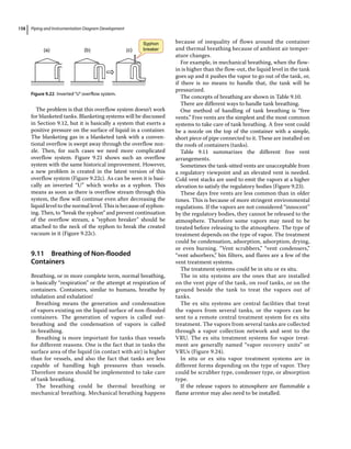
74. Principles of PID Development 55
the flow rates that fail to fill the cylinder of the pump in
one stroke. Partial filling of the cylinder may cause some
damage to mechanical components of the pump in the
long term. This minimum flow is a function of cylinder
volume and stroke speed of a specific pump.
The TDR of a pipe is a bit more complicated. Here the
minimum flow should be defined as the minimum flow
that does not fall into laminar flow, or the minimum flow
that keeps a check valve open. For liquid flows in pipes,
the minimum flow can be interpreted as the minimum
flow that makes the pipe seal (no partial flow pipe)
because a flow smaller than that will freeze in an outdoor
pipe. If the flow contains suspended solids, the minimum
flow should prevent the sedimentation of suspended
solids.
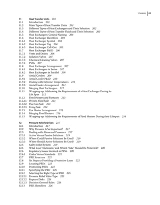
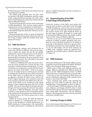
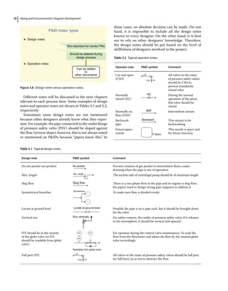
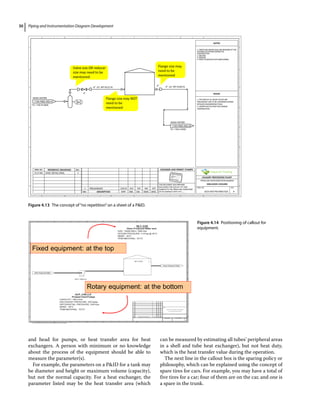
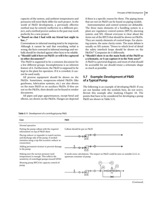
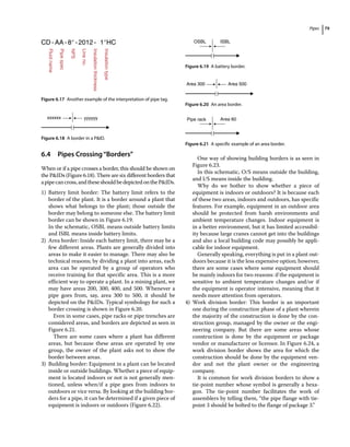
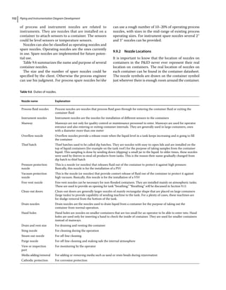
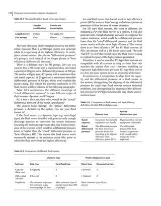
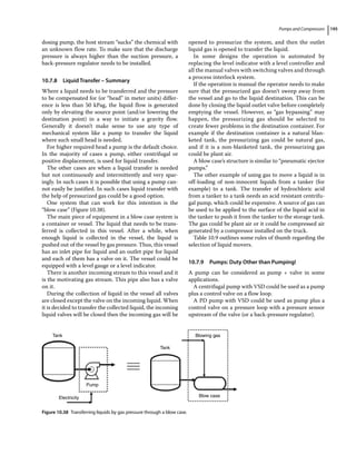
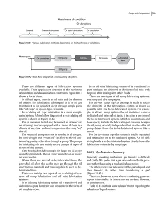
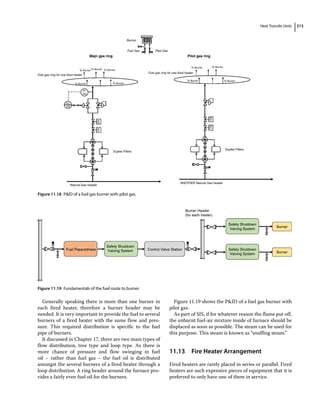
Table 5.5 is a table of typical TDR of some equipment.
Table 5.6 shows the large TDR of storage containers.
The high TDR of these items also explains why contain-
ers are used for surge dampening in plant‐wide control
practices.
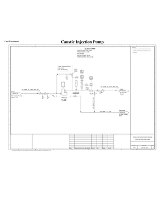
In some cases, deciding on the required TDR needs
additional consideration. One example is a chemical
injection package. TDR is important for chemical injec-
tion packages to ensure that there is no time that chemi-
cal overdoses or underdoses happen, if both of them are
intolerable to the process.
It is popular to expect to see a chemical injection pack-
age provide a TDR of about 100:1 or lower; possibly 10:1
can be provided by stroke adjustment and another 10:1
through VFD. But why is such large TDR is necessary if
the host flow experiences only 2:1? This huge TDR is
generally because of the uncertainty in required chemi-
cal dosage and abundance of chemical producers. If the
dosage is fairly firm and the chemical is a nonproprietary
type, the TDR can be decreased to lower the cost of the
chemical injection system.
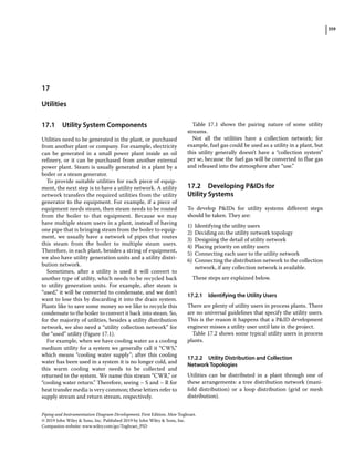
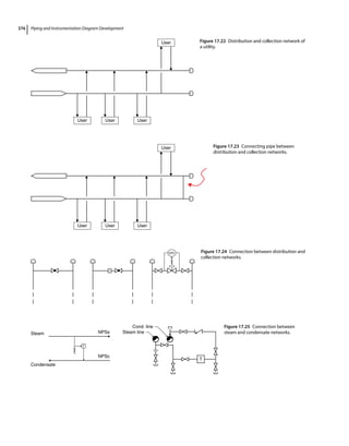
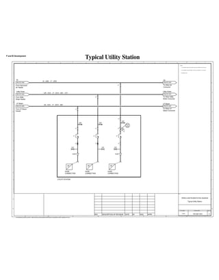
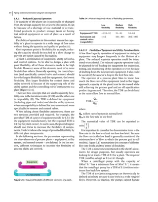
5.4.2.1.2 Flexibility of Utility Networks
The flexibility of utility networks is also defined by TDR.
As mentioned, when a TDR of, for example, 2/1 in a plant
is requested, the TDR of utility network should be higher.
As the utility system needs a large TDR, it generally
needs a container in the utility production area to absorb
the fluctuations caused by the utility usage change in
process areas. Table 5.6 shows the name of these surge
containers in different utility systems.
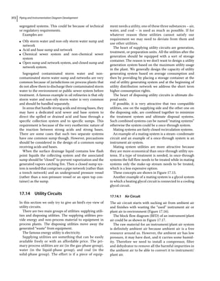
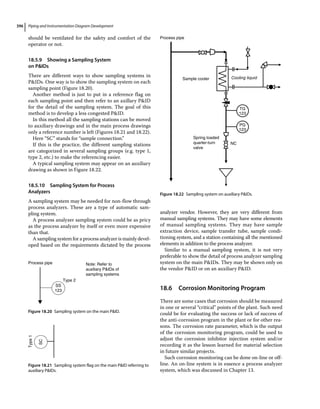
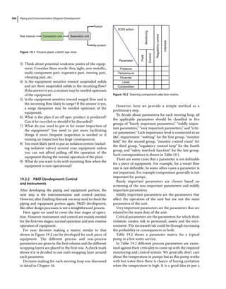
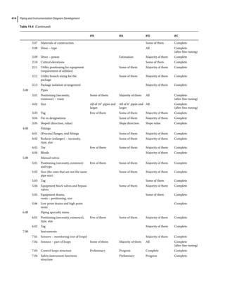
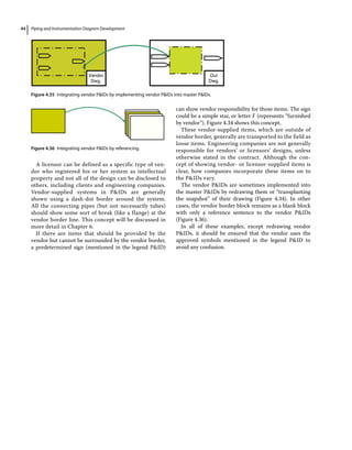
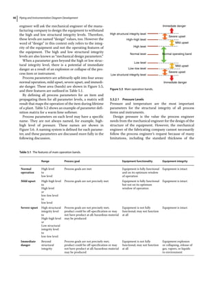
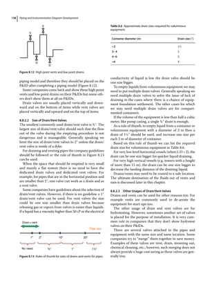
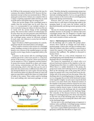
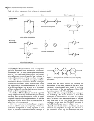
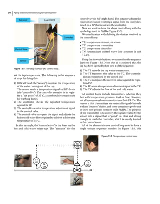
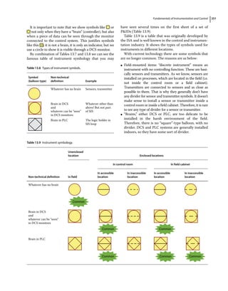
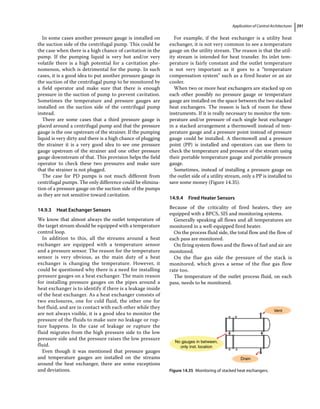
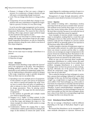
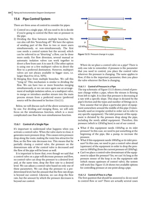
The utility network by itself experiences different levels
of turndown, and consequently it needs different TDR. The
main header can need the minimum TDR, whereas the
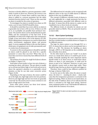
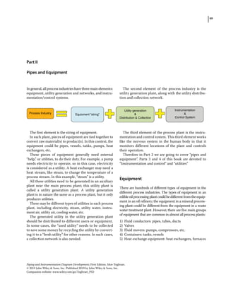
subheads may need a higher or lower ratio (Figure 5.18).
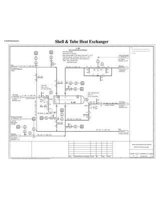
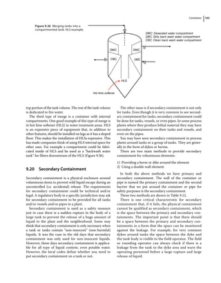
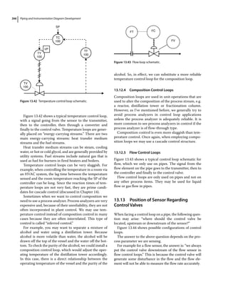
Achieving a high TDR for the utility network and
instruments is not difficult. The utility network is mainly
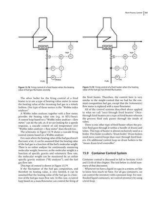
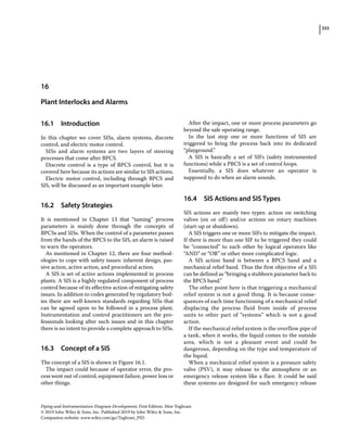
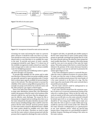
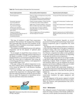
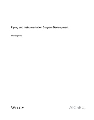
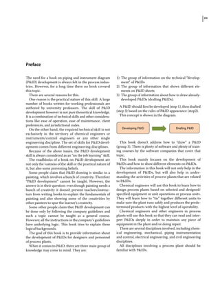
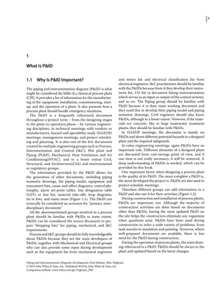
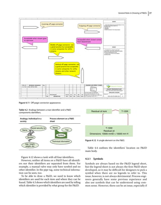
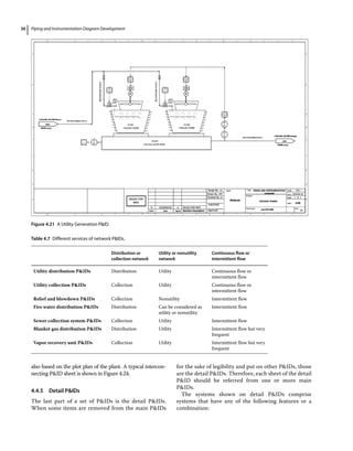
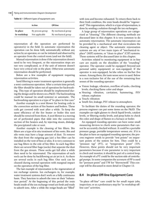
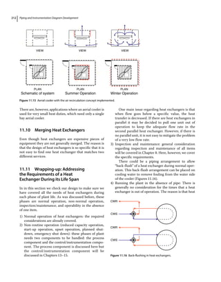
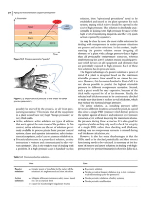
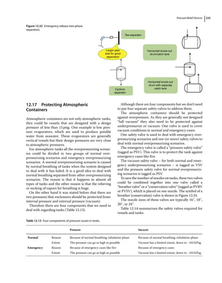
Mechanical relief action
Mechanical relief action
SlS action
SlS action
Alarm
Alarm
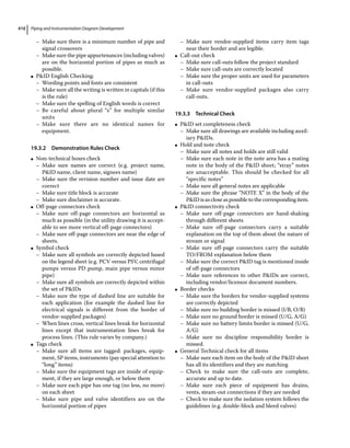
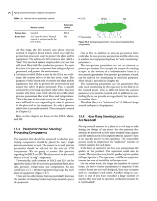
BPCS actions
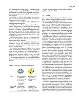
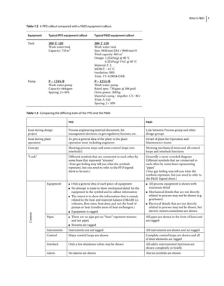
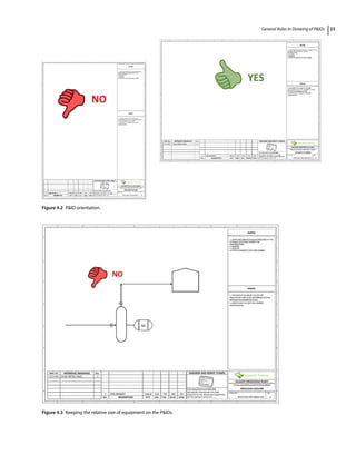
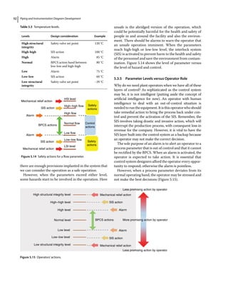
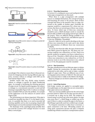
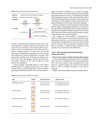
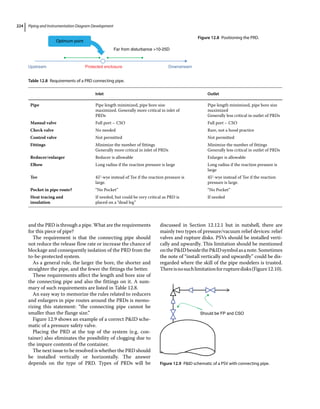
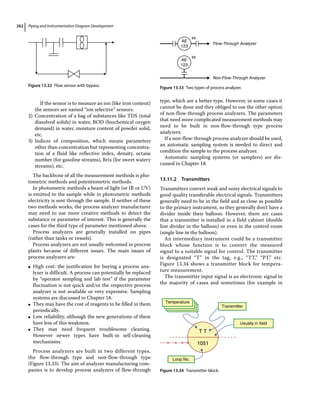
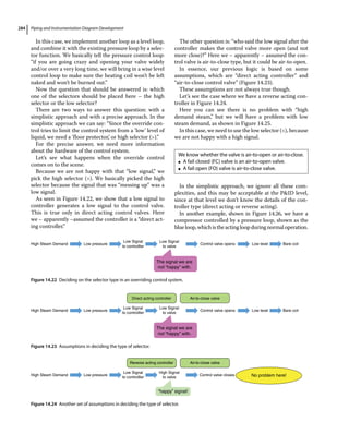
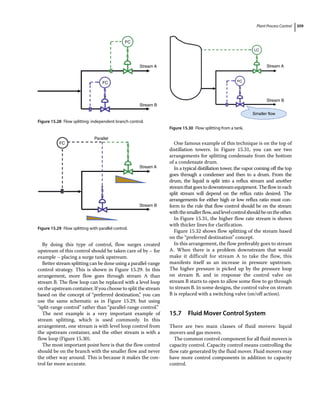
High–high flow
HSl level
High flow
Normal flow
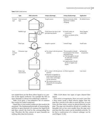
Low flow
Turn-
down
ratio
(TDR)
Low–low flow
LSI level
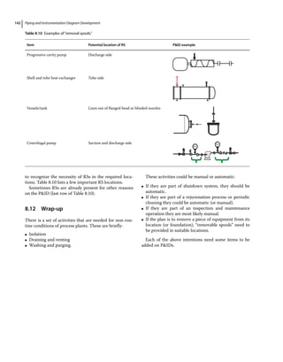
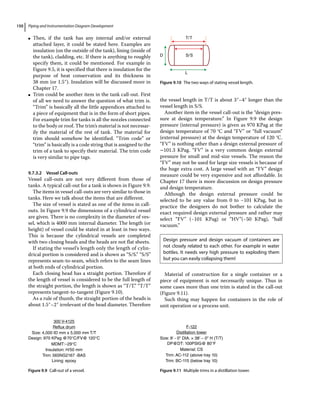
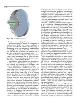
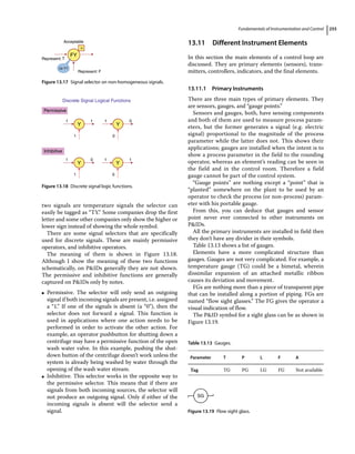
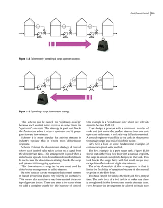
Figure 5.17 Concept of turndown ratio.
Table 5.5 Turndown ratio of some selected equipment.
Item Turndown ratio
Pipe Large but depends on the definition of
maximum and minimum flow.
Storage
containers
(tanks or
vessels)
Very large (maximum is total volume of the
container, but minimum could be dictated by
downstream item. For example a centrifugal
pump dictates a minimum volume to provide
required net positive suction head [NPSH]).
Centrifugal
pump
Typically 3:1–5:1
PD pump Theoretically Infinite
Heat
exchanger
Small, depends on the type (e.g. less than
1.5:1)
Burner Depends on the type between 2:1 to 8:1
Table 5.6 Utility surge container to provide turndown ratio.
Utility Surge container
Instrument air (IA) Air receiver
Utility water (UW) Water tank
Utility steam (US) Steam drum in conventional
boilers (in steam generators
cannot be stored; the system
design should be in a way to
“float” US with other streams.
Utility air (UA) No dedicated container can
“float” with IA
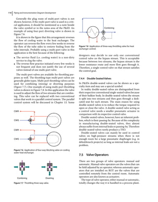
Cooling water (CW) Cooling tower basin
Cooling or heating
glycol
Expansion drum

75. Piping and Instrumentation Diagram Development
56
composed of pipe circuits, which inherently have long
TDR, and instruments (control valves and sensors) have
intrinsically large TDR generally better than 20:1.
5.4.2.1.3 Flexibility of Control Valves and Sensors:
Rangeability
Instruments have a higher level of responsibility than the
equipment and the utility network because their duty is
not limited to normal operation or a band of low to high
levels. They have to be operational in a wider band of
low‐low to high‐high. Therefore, rangeability can be
defined as:
R
Q
Q
Hi Hi
LoLo
where QHi Hi is flow rate of an instrument or control
valve in high‐high level and QLo Lo is the flow rate in low‐
low level.
Table 5.7 is a table of typical rangeability of some
instruments.
5.4.2.1.4 Providing Required Flexibility
There are three main ways that specific flexibility for
plant items can be given: by using items with inherently
high flexibility, placing similar items with a smaller
capacity in parallel, and providing a recirculation route.
One example of using recirculation to provide enough
TDR is the minimum flow line for centrifugal pumps.
Using multiple pieces of equipment in a parallel series to
provide enough TDR is popular in designing sand filters
in the water treatment industry.
1) Using equipment that has inherently higher flexibility.
There are some process elements that have inherently
higher flexibility such as tanks and pipes.
It is not always easy to recognize if a piece of equip-
ment has inherently high or low TDR; however, there
are some guidelines that can be used to determine
this:
–
– Small volume equipment have a slimmer TDR than
larger volume equipment
–
– Equipment with internal baffles (compartmented)
have lower TDR.
An example of this is some gravity separators such
as oil–water separators.
–
– Equipment in gas services may show higher TDR
than the ones in liquid services.
–
– Equipment with internal weir (especially fixed
ones) may have very low TDR.
–
– Equipment that uses some properties of inflow for
its functioning may have lower TDR. Examples are
a cyclone and hydrocyclone. In cyclones, the energy
of the flow is used to generate centrifugal force; less
flow causes less centrifugal force and that may cause
an ineffective system. Another example is conven-
tional burners; the lower fuel to a burner may cause
short flame or even back fire in the burner.
The utility network should have a large TDR, and
they are mainly comprised of pipes in different sizes.
If a control valve is necessary in the network, some-
times it may need to have parallel control valves with
split control because of the large required TDR.
–
– Equipment containing loose porous media may
show lower TDR in liquid services. And the TDR
may be lower when the porous media is built with
larger particles.
Examples of these types of equipment are sand fil-
tration, catalyst contactors, and the like.
Instruments generally have an inherently high
rangeability, which satisfies the plant requirements
most of the time.
2) Using parallel equipment.
Instead of using equipment with the capacity of
100m3
h−1
, use an arrangement of two parallel equip-
ment each with the capacity of 50m3
h−1
By doing
this, a TDR of at least 2:1 can be used (at least because
the equipment may have inherent RDR capability that
may be added to the provided 2:1 TDR).
By using three, 33m3
h−1
pieces of equipment in a
parallel arrangement, a better TDR of 3:1 can be
achieved. This technique has other benefits; the parallel
arrangement provides higher availability for the system
because losing two or three parallel equipment is less
probable that losing just one. Instruments generally
Low turndown ratio
High turndown ratio
Figure 5.18 Map of turndown ratio for a typical utility network.
Table 5.7 Turndown ratio of selected instruments.
Item Turndown ratio
Flow
meter
Depends on type and between 3:1 to 50:1 and
more.
Control
valve
Depends on type and the characteristics, generally
50:1, and less than 100:1

76. Principles of PID Development 57
have a high and suitable flexibility (rangeability). But if
their rangeability is not enough, generally using them in
parallel is the solution. For example, using two control
valves in parallel in a single control loop of “split range”
is example of this technique. However, there are some
disadvantages involved, including the increase in the
capital cost and operating cost.
3) Providing recirculation pipe.
This method is exclusively used for noninstrument
items. Implementing a recirculation pipe from an equip-
ment outlet to its inlet is a popular method to increase
the TDR of a system. The recirculation pipe may need
some control system placed on it to prevent full flow
backward. An example is using a minimum flow line for
a centrifugal pump. A centrifugal pump with the capac-
ity of 100m3
h−1
and a minimum flow of 30m3
h−1
(i.e. a
TDR of 1:3) can be equipped with a minimum flow line
with an appropriate control system to increase its TDR
(Figure 5.23). If the minimum flow line and the control
system are designed to handle a maximum 30m3
h−1
, it
means that the TDR of the pump is theoretically
increased to infinite by zeroing the minimum flow.
However, this method cannot be applied to all types of
equipment. For example, this is not a good technique
to increase the TDR of a furnace or fired heater;
recirculation of fluid around a furnace may increase the
furnace coil temperature, causing it to burn out.
5.4.3 Reduced Efficiency Operation
Reduced efficiency of a piece of equipment or unit may
generate low‐quality or off‐specification products.
If the quality of product is still acceptable, nothing can
be done. Also nothing can be done if there is already a
higher‐than‐needed quality product mixed the low‐­
quality product because this still creates an acceptable
product. In this case, though, a product tank (or any
other product bulk system) is needed to allow the mixing
of high‐quality with low‐quality products.
The low‐quality products can be routed back to an
upstream point to reprocess them to get acceptable
products. They can also be redirected to an off‐specifica-
tion tank and then mixed gradually with overly high‐
quality product. The low‐quality products can be routed
to an off‐specification tank to rerun the batch and turn it
into high‐quality product, returning it back to the system
when complete. Low‐quality products can also be sold to
a third party for further processing to attain the high‐
quality product or other marketable product. Table 5.8
outlines these techniques.
Table 5.8 Options for dealing with a low‐efficiency operation.
Option Schematic
1 Do nothing! No schematic; no any specific addition to
PID
2 Recirculating the off‐specification
product to upstream unit
Feed
Off-spec. product
Unit
3 Redirecting the off‐specification
product to an off‐specification tank
and then returned gradually
Feed
Reservoir
Unit
Off-spec.
product
4 Redirecting the off‐specification
product to an off‐specification
tank, retreat it (by batches) and
then return it
Feed
Reservoir
and
treatment
Unit
Off-spec.
product
5 Redirecting the off‐specification
product to an off‐specification tank
and then sell it to a third party for
retreating it or selling as is
Feed
Reservoir
Unit
Off-spec.
product

77. Piping and Instrumentation Diagram Development
58
These actions can be done manually after an operator
or an automatic control system checks the quality of the
product. Any of the aforementioned solutions can be
used. However, the more important point is that the
cases of low‐efficiency operation should be considered
for each unit that creates a physical or chemical change
on the process stream.
5.4.4 Start‐Up Operations
There are at least two types of start‐up operations: the
first start‐up of a plant after its construction, which is
called commissioning, and the start‐ups after each
shutdown.
The start‐ups after shutdowns can be in two different
types: start‐up after a planned shutdown and start‐up
after emergency shutdowns. A start‐up after an emer-
gency shutdown may have more steps than a start‐up
after a planned shutdown.
Start‐up operations can be assumed to be a severe
capacity reduction case. In this situation, not all the
instruments will work properly because process param-
eters during the start‐up are not necessarily within
their range. However, the operating personnel who are
attending the plant are the resources available and
expected to compensate for the lack of instrument
operability. They will be present as a larger group dur-
ing normal operation.
The commissioning operation is a specific case of a
start‐up. In addition to all issues related to a start‐up, a
commissioning has many other problems related with
poor construction and installation. During the plant
construction, the electric motors may be connected to
Mechanical relief action
Mechanical relief action
SlS action
SlS action
Alarm
Alarm
BPCS actions
High–high flow
HSl level
High flow
Rangeability
(R)
Normal flow
Low flow
Low–low flow
LSI level
Figure 5.19 Concept of rangeability.
Unit
Unit
Vs.
Unit
Figure 5.20 Using parallel equipment to provide a required
turndown ratio.
FC
Split range 0 – 50%
50 – 100%
Figure 5.21 A control valve arrangement in wide rangeability
requirement.
Vs.
Recirculation pump
Unit
Unit
Figure 5.22 Recirculating for increasing TDR.
FC
Figure 5.23 A centrifugal pump minimum flow recirculation to
increase TDR.

78. Principles of PID Development 59
rotate in reverse, the bolts may not be fastened enough,
thus leaking, and there can be a junk left inside pipes.
A good PID should take care of these issues, too. For
example, a temporary suction strainer (TSS) can be
installed on the suction side of centrifugal pumps to
protect the impeller from incoming debris during com-
missioning. The strainers should be removed from the
pipe later.
A general procedure for starting up of a process equip-
ment is as follows:
●
● Venting or draining the system: A system ready to be
started can be filled with process fluid (gas or liquid), it
can be empty, or it can be filled with air. In any case,
the system should be empty at the start.
●
● Inerting: This step can be skipped in some cases. The
goal is to replace any dangerous atmosphere with an
inert and readily removable atmosphere. This is done
by introducing an inert gas to the piece of equipment.
●
● Warming up: This step is needed if the operation tem-
perature of the piece of equipment is different than the
ambient temperature. To do this, a small amount
of process fluid is allowed to into the piece of
equipment.
●
● Partial loading and recirculation: Start‐up operations
can be done by recirculation. Figure 5.24 shows the
basics of this procedure.
If the system is not reversible, the start‐up operation
can be more complicated and case specific.
If the start‐up procedure goes through the recircula-
tion (which is not a rare case), the highest attempt
should be made to avoid using a long pipe for the pur-
pose of start‐up. It is not a sound decision to spend lots
of money for the pipe that is supposed to be used only
during the start‐up. As much as possible, the existing
pipe arrangement should be used for the purpose of
start‐up recirculation, especially when a high‐bore
pipe is needed.
The tendency of using the piping arrangement, which
was implemented for normal operation, for the purpose
of start‐up recirculation is so strong that some process
engineers forget to think about the start‐up operation
during the development of the PID and assume that
they will find a way to accommodate start‐up somehow.
5.4.5 Shutdown
There are two types of plant shutdown: planned and
emergency. The goal of a shutdown is stopping the
­
production of a plant or a unit. However, a planned
shutdown happens based on a prior decision and prepa-
rations, whereas an emergency shutdown occurs because
of ­
circumstances beyond anyone’s control.
The aims of a planned shutdown are upholding oper-
ators’ safety, protecting the hardware asset, and mini-
mizing or preventing product loss. The restart‐up after a
planned shutdown is easy.
An emergency shutdown has the same aims; however,
minimizing or preventing product loss may not be
achievable. One aim of the interlock system is to
­
complete an emergency shutdown in a way similar to a
planned shutdown. During an emergency shutdown, the
main driver of a process plant can be interlock system
(SIS) because in such situations, the operator’s actions
are not reliable.
The reasons for an emergency shutdown are diverse.
However, because every process plant operates based on
cooperation among the elements of equipment, utility
system, and instrumentation and control system, an
emergency shutdown can be classified based on the fail-
ure of each those elements. The error by operators or
other plant personnel is the fourth source of emergency
shutdown.
Failure or rupture of a tank may lead to an emergency
shutdown. Fire in a limited area of a plant may also lead to
an emergency shutdown because of failure in equipment,
utility network, or instrumentation and control system.
One very common emergency shutdown is because of
utility failures. For example, an electricity blackout may
cause an emergency shutdown. In many cases, an emer-
gency shutdown leaves stopped equipment with fluid
contained in them. Such a situation is considered poten-
tially problematic. The main issue about equipment with
fluid in it is setting the fluid inside of the equipment,
making it difficult to restart it.
A winterization concept should be implemented when
developing the PID to deal with this issue. Contrary to
the word winterization, it is not limited to winter time.
Using a winterization tries to prevent the settling of
remained fluid in a piece of equipment because of low
Unit
Normally closed will
be open only for
starting up
Figure 5.24 General procedure for starting up a unit.

79. Piping and Instrumentation Diagram Development
60
temperature, regardless of the season. Winterization will
be discussed in more detail in Chapter 17.
If the equipment cannot emptied, it should be checked
to ensure that the remaining fluid does not create any
problems for restarting the equipment. Restart after a
shutdown is not always easy, and several steps may be
taken to start the plant again.
If high‐inertia equipment continues to run after emer-
gency shutdown, this may cause a problem. For example,
a large centrifugal compressor will be left with rotating
impeller on for several minutes after an emergency shut-
down. During PID development, an available system to
continue the lubrication of the centrifugal compressor
needs to be planned; otherwise, the compressor bearing
may fail quickly.
To summarize, in developing the PID to cover the
shutdown stage of a process plant, a good interlock sys-
tem and winterization, among other project‐specific
items, should be implemented.
5.4.6 Inspection and Maintenance
Inspection, rejuvenation, and maintenance includes a
wide range of activities that will be discussed more in
detail in Chapter 8. Here, this topic is briefly covered.
Because plant items are not eternal, they should be
inspected, and if they need rejuvenation or maintenance,
it should be performed.
Maintenance or rejuvenation can be triggered by any
of three situations: after failure, based on inspection, and
based on time intervals. The first one is termed correc-
tive maintenance; the second one is inspection‐based
preventive maintenance; and the third is time‐based pre-
ventive maintenance.
Therefore, two stages of a process plant are revealed:
inspection and maintenance and the time that a compo-
nent is out of operation because of maintenance. In this
section, the inspection and maintenance are covered,
and in the next section, the period of time an item is out
of operation because of maintenance is discussed.
During PID development, provisions allowing easy
inspection and maintenance should be included.
This stage of the process plant is applicable again to
the equipment, control system, and utility system, and it
needs to be determined which equipment or system
needs maintenance at what frequency and how long it
takes to maintain it. These questions can be answered
quantitatively or qualitatively.
5.4.6.1 Quantitative Approach to Maintenance
Requirement
Answering these questions needs a vast amount of
knowledge, which is generally the territory of a mechani-
cal integrity engineer. However, there are two important
parameters: mean time between failure (MTBF) of the
equipment and mean time to repair (MTTR) the equip-
ment. These two parameters specify the availability of a
piece of equipment.
Table 5.9 outlines some typical values of MTBF and
MTTR for a few items. This table shows that, for exam-
ple, a typical centrifugal pump will fail every 1 to 3 years,
and its maintenance may take between 8 and 16hours.
It is important to know that there is no unique value
for MTBF and MTTR of centrifugal pumps. The param-
eters depend on the pump manufacturer, the type of pro-
cess plant, the environmental parameters (ambient
temperature, air humidity, etc.), and also the skill level of
personnel. Each company may have their own database
to collect the data and estimate MTBF and MTTR of
their equipment and instruments.
5.4.6.2 Qualitative Approach to Maintenance
Requirement
During PID development, a qualitative approach to
the maintenance requirement is needed as it provide a
bigger perspective encompassing all equipment, espe-
cially for the expensive ones. Here is a question we try
to answer qualitatively: what equipment needs more
maintenance?
In process plants, inspection is done on any or all of
the features of a piece of equipment, for example, pro-
cess goal, equipment functionality, and equipment integ-
rity. This means that during inspection, we check if the
process is running smoothly, if a piece of equipment is
functional, or if there is no breakage in the equipment.
The answer can be provided for each goal of inspection:
process, equipment functionality, and equipment integrity.
For the processes that are based on a more probabilis-
tic phenomenon, they may need more frequent inspec-
tions. The examples are burners and vessels that contain
media like sand filters.
A peep hole is generally provided to observe the exist-
ent of flames in burners and sight glasses on the vessels
with media.
For equipment functionality and integrity, the answer
depends on the equipment and the process condition.
It means some equipment inherently needs more
­
maintenance attention, and some process conditions
Table 5.9 Some typical values of MTBF and MTTR for three items.
MTBF (yr) MTTR (hr)
Centrifugal pump 1–3 8–16
Centrifugal compressor 10–20 6–24
Shell and tube heat exchanger 10–20 16–72
MTBF, mean time between failure; MTTR, mean time to repair.

80. Principles of PID Development 61
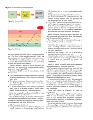
make the equipment needier for maintenance. These
two components are discussed next.
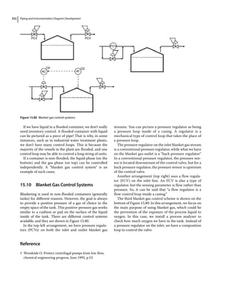
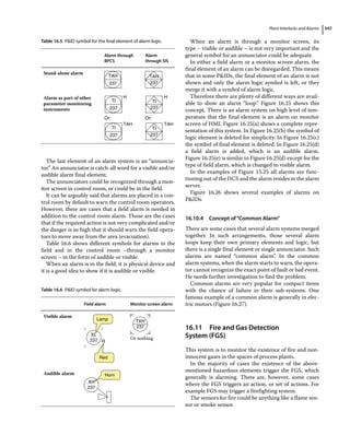
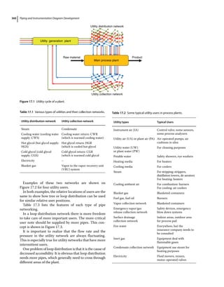
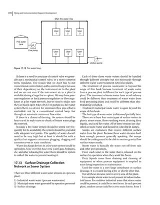
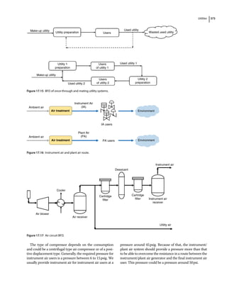
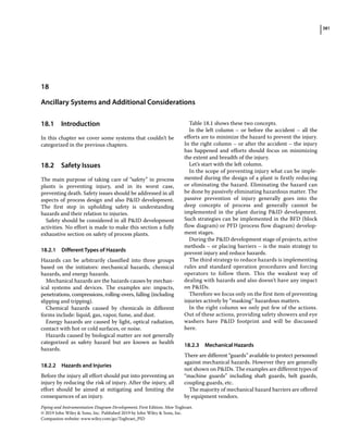
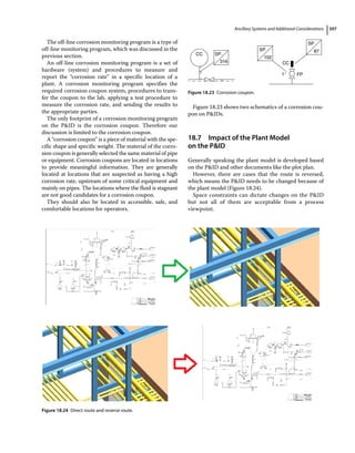
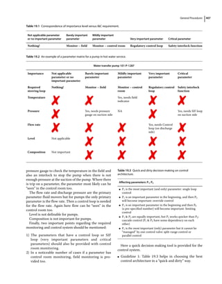
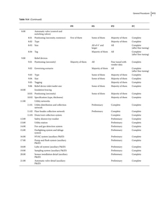
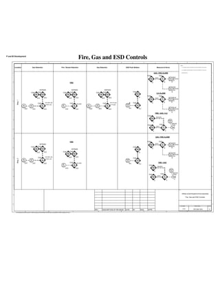
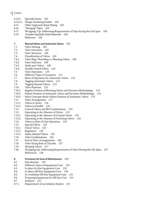
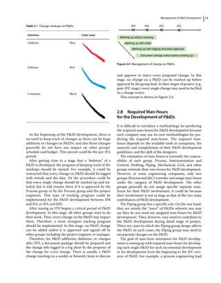
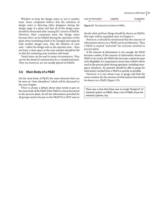
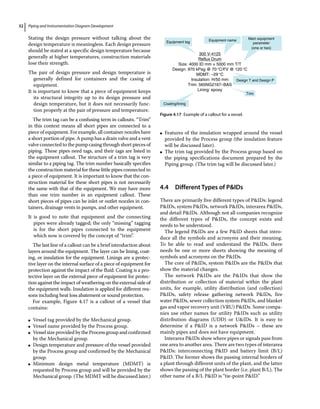
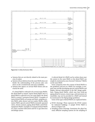
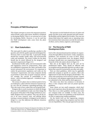
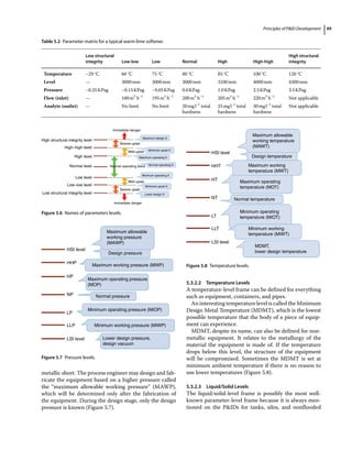
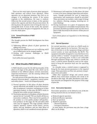
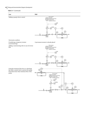
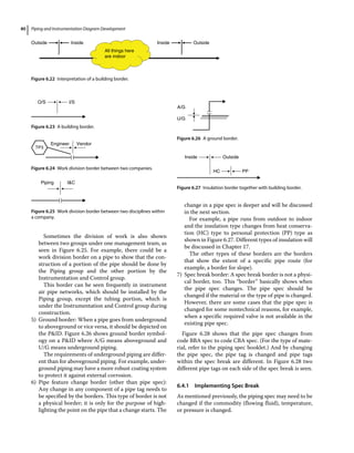
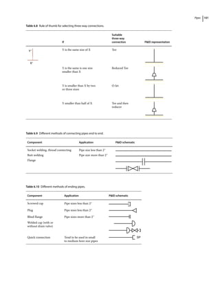
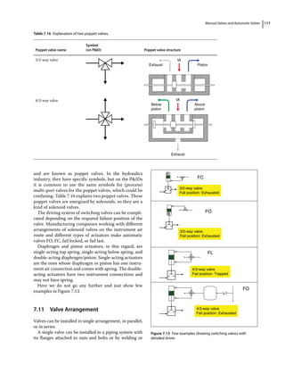
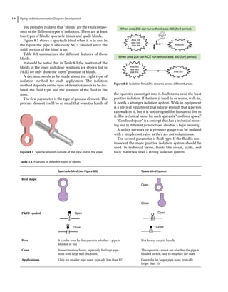
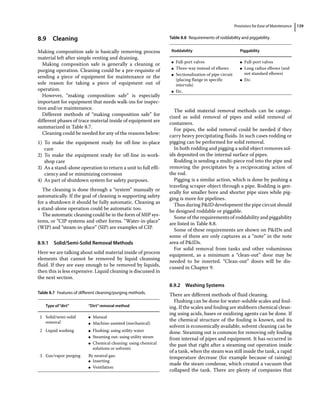
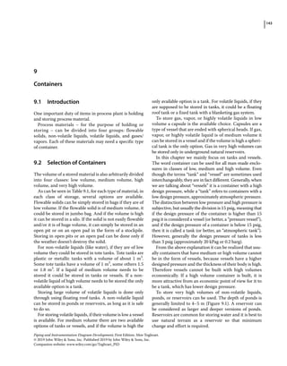
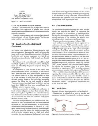
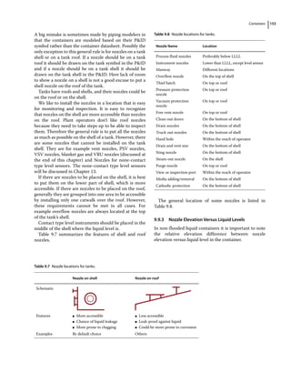
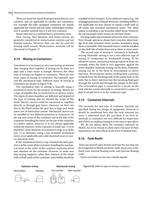
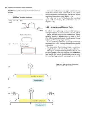
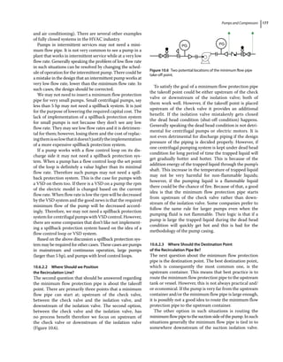
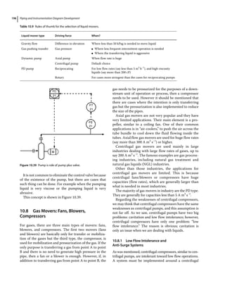
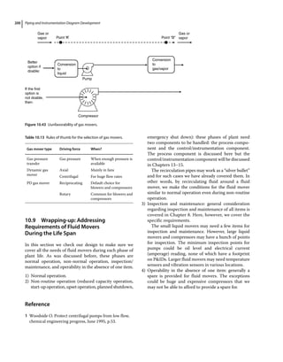
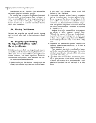
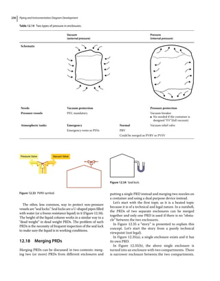
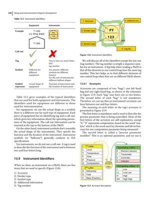
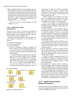
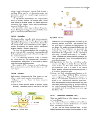
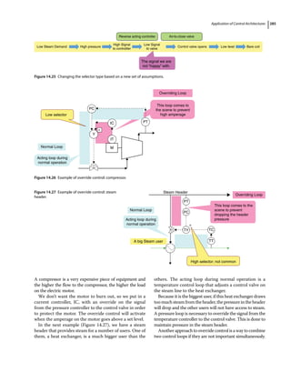
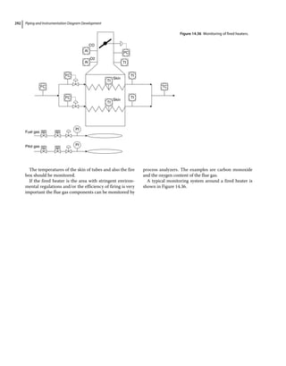
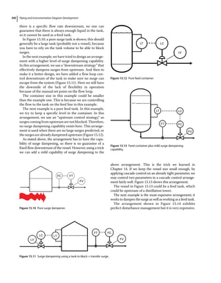
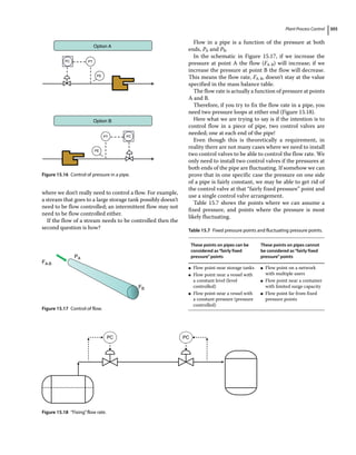
The equipment that are static generally need less
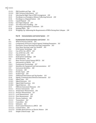
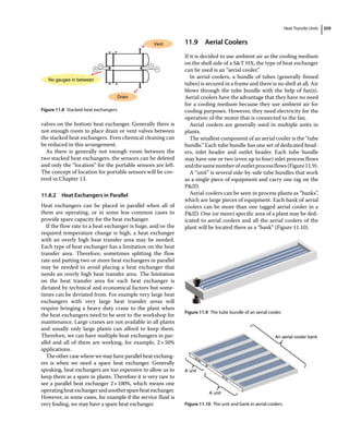
maintenance. Among nonstatic equipment (i.e. dynamic
equipment), the ones with linear (reciprocating) move-
ments may need more maintenance attention than the
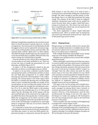
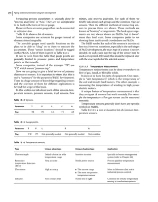
ones with rotary movements (Figure 5.25).
Where there is a rotating shaft in a piece of equipment,
the high rotational speed shafts (high revolutions per
minute [RPMs]) may need more maintenance attention
than low RPM shafts. Pieces of equipment that have tight
clearances may need more inspection and maintenance.
This is especially true if they are being used in services
that are not clean.
When it comes to process and process conditions, the
equipment that works in very high or very low tempera-
tures or pressures may need more maintenance atten-
tion. The equipment that processes non‐innocent fluids
(i.e. highly acidic, precipitating, scaling, fouling, or any
other aggressive fluid) may need more maintenance
attention.
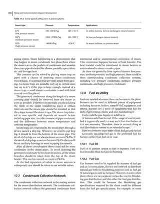
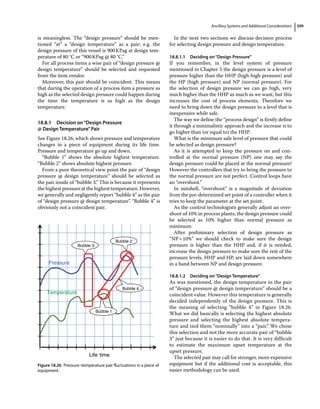
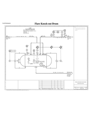
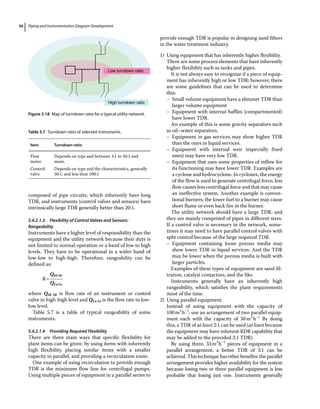
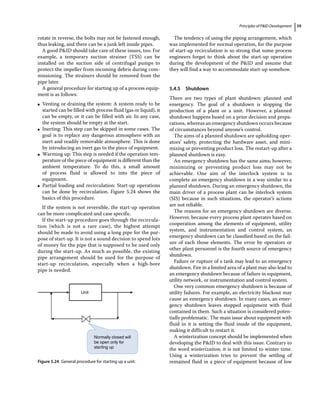
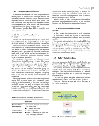
5.4.7 Operability in Absence of One Item
The designer needs to decide the repercussions of equip-
ment loss, which means in the absence of a piece of
equipment, it needs to be decided what will happen to
the rest of unit or plant. The wide range of answers and
decisions include:
1) Do nothing! In this case, the piece of equipment,
unit, or even plant should shut down in the absence of
a piece of equipment or instrument. This option
should be avoided. Sometimes it is inevitable when a
piece of equipment of interest is the main or one of
the main pieces of equipment of the plant.
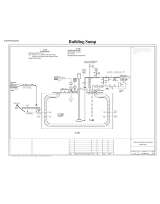
2) Accumulation of fluid in middle containers. In this
solution, placing two containers with enough resi-
dence times upstream and downstream of the absent
component help to prevent the absence of the compo-
nent get “visible” by the rest of plant. In this solution,
the upstream container allows the accumulation of
fluid, and the downstream container provides flow for
the downstream units.
3) Redirecting the in‐flow to a “reservoir” for later
usage. In this solution, the feed to the equipment can
be redirected to a temporary reservoir (like waste
tank or pond) to be processed later by returning it
back to the system. Usually this is solution is not avail-
able for gases or vapors.
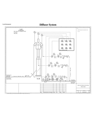
4) Redirecting the in‐flow to an “ultimate disposal”
system. This solution is the same as previous one, but
the flow sent to the external reservoir cannot be
returned. The feed to the equipment can redirected
to a waste‐receiving system, like a flare system. This
option can be considered if the preceding option is
not doable. The previous option is definitely a better
option because valuable materials are not lost.
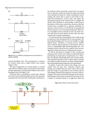
5) Bypassing the absent item. The feed to the equip-
ment can be bypassed temporarily with marginal
impact on the operation of the system, like bypass-
ing a trim heater if being off‐temperature does not
hurt the plant for a short time. There are some cases
that is decided to bypass the equipment or unit when
it is out of operation. This can be done if the lack of
equipment or unit does not affect the process in the
short term.
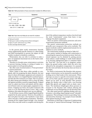
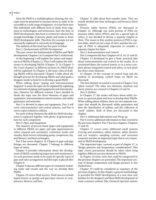
6) The nearly “similar” item in parallel. A nearly simi-
lar system in parallel can take care of the flow that
used to go to the absent system but not necessarily
with the same quality. One example is having a man-
ual throttling valve (e.g. globe valve) in a bypass loop
of a control valve. The other example is placing a
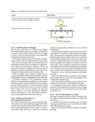
bypass pipe for a pressure safety valve (PSV) together
with a pressure gauge (or pressure gauge point) and a
globe valve. In the case of pulling the PSV out of oper-
ation, an operator will act as a PSV by monitoring the
pressure of the container and being prepared to open
the valve if it is needed.
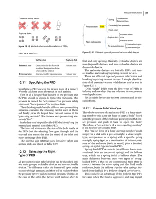
7) The exact “similar” item in parallel. A parallel,
exact replica as spare system can take care of the flow
that used to go to the absent system. This is the most
expensive option. The examples are all spare pumps
or spare heat exchangers (in very fouling services).
Spare equipment are very common for fluid‐moving
equipment as usually the pumps and compressors
cannot be handled otherwise. One important exam-
ple is having two fire pumps in parallel with two dif-
ferent types of drives (i.e. one electromotor and the
other one a diesel drive pump). The spare can be in
different forms.
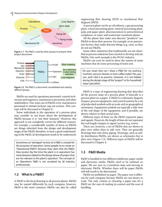
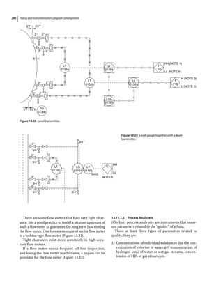
In Table 5.10, the schematics of these options in the
PID are shown.
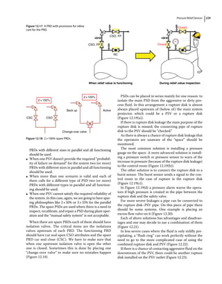
5.4.8 Provision for the Future
The other concept that may affect the development of
the PIDs are provisions for the future. The future
arrangement of a plant is not necessarily similar to the
current arrangement of plant because the future of a
market is not always foreseeable, or if it is foreseeable, it
is not economically justifiable to incorporate it into the
current plant design. However, to minimize the cost of
rearrangement of a plant in the future, some items can be
placed in the plant design and the PID. Therefore,
some “footprints” of future on a PID may be seen; how-
ever, not all plants consider the future.

81. Piping and Instrumentation Diagram Development
62
The future programs can be a planned or unplanned
program. A planned change in a process plant could be
scheduled or unscheduled and yet still be a foreseeable
change.
Different words are used to describe a planned future
program. Revamping is a general term that refers to any
change to a plant. Upgrading means implementing new
inventions or practices to decrease the operating cost or
increase the quality of product(s). Retrofitting means
adding new features to the plant to produce additional
products, better products, or the same product at lower
cost or with less safety concerns. Retrofitting can be
needed because of a change in feed type. Expansion
means increasing a plant capacity to match the new
Table 5.10 Options for dealing with lack of a component.
Option Schematic PID example
1 The lack of item does not generate
any upset in the rest of plant or
whole plant should be shut down Steam
generator
2 The upstream tank stores the flow
in and the downstream tank
provides flow out for a short period
of time
Furnace
3 Redirecting the in‐flow to a
reservoir for later sending it back
Reservoir
Pond
4 The flow‐in is sent permanently for
ultimate disposal and the stream
will be wasted
Ultimate disposal
To flare
5 Bypassing the absent item
Bypass
6 The similar item in parallel
7 The exact replica in parallel

82. Principles of PID Development 63
requirements of the market. Expansion can also be
scheduled on a specific date in future or unscheduled
whenever the market picks up and needs more of a par-
ticular product. Expansion can be done by adding a new
“train” or adding or upsizing several (hopefully not all)
pieces of equipment. In this context, a train is a similar
plant with the same capacity next to the original plant
and which may share some of the same resources as the
original plant. A plant can be designed and built based
on the training concept because of a limited available
budget or other reasons. Different trains of a plant may
have cross piping to each other to increase the reliability
of the plant (Figure 5.26).
It is very common that multiple trains of a plant share
the same utility system (including utility generation plant
and utility distribution and collection network). In such
cases, all the utility generation plant (e.g. boilers, coolers,
potable treatment package, utility networks) should be
upsized, and the utility network be ready and extended
through the future train. The upsized pipes may have
plenty of blind flanges at different locations of utility net-
works and process headers.
An unplanned future program is categorized in all
debottleneck activities, rehabilitation, or optimization.
No design is perfect, and to bring a plant design even
near perfection may lengthen the project duration
beyond economically accepted measures. Therefore,
almost always, the designers do their best to design a
plant within the allotted time for the design, and they
leave the additional fine‐tuning for later and after
start‐up of the plant. There is a better chance to fine‐
tune a design during the operations of a plant rather
than before its start‐up. However, a specific debottle-
neck activity is not always needed; there are cases in
which the plant owners are comfortable with the design
and they do not do any debottlenecking on the plant
currently operating.
Rehabilitation is one common example of an
unplanned future program. Rehabilitation means
replacing old equipment with new equipment or
refurbishing old equipment for the purpose of decreas-
ing the operating cost or increasing the quality of
products.
Unplanned future programs do not have any footprint
on a PID until they are initiated.
5.5 ­
Conflicting Check and Merging
Opportunities Check
This step has two substeps: checking if a conflict is result
of the functionality of added items and checking if some
of added items can be merged into one item to save
money.
5.5.1 Conflict Check
This step is making sure that no added element within
one stage of the plant’s life cycle jeopardizes another
item’s goal. For example, adding a bypass with a manual
block valve for a safety‐related switching valve for the
purpose of making the plant operational when the
switching valve is out for maintenance (point 5) could
jeopardize the intent of the switching valve’s operation in
a safety instrumented system (the bypass could left open
and therefore is a safety flaw).
5.5.2 Merging Opportunities Check
Merging can be done in two different levels: merging dif-
ferent components including equipment, containers,
pipes, or instrument or merging different items on one
specific component. The former is the opportunity to
use one pump, instead of two pumps, to handle two ser-
vices. The latter is the opportunity to use one nozzle on
a tank as an overflow nozzle and vent nozzle.
This step is deciding whether the added items or com-
ponents can be merged with each other. This is checking
if a single shared item or component can address multi-
ple requirements of the different plant life cycles or not.
The quick answer to this question is to merge the items
or components and use the time‐shared item as much as
possible to save money. In simpler terms, for the sake of
saving capital and operational costs, the required items
or components should be shared. It is better to put more
than one duty as much as possible on the shoulders of
each added item or components. However, shared items
are more difficult to fit into the design, may be confusing
to operators, are more prone to cross‐contamination,
and can generate a big shutdown caused by a small ­failure
(redundancy issue).
A common example of merging multiple components
in a plant happens in batches and intermittent opera-
tions. If you have a pump operating in an intermittent
mode, you may be able to put another duty on the
­
shoulder of this pump when it is freed from its main
duty. It means that some components in such operations
can be used for different duties in different time spans.
Merging items are doable when one item is function-
ing in a time phase other than that of the similar item.
Static equipment
Dynamic items: Rotary equipment
Dynamic items: reciprocating equipment
Figure 5.25 Necessity of inspection and maintenance for
equipment.

83. Piping and Instrumentation Diagram Development
64
For example, if an item was added only for the ease of
maintenance, another duty may be placed on its shoul-
ders during normal operation.
Later in this book, each piece of equipment and oppor-
tunities for merging them are discussed.
5.6 ­Dealing with Common
Challenges in PID Development
During the development of a PID there are occasion-
ally some challenges to find a better option among the
available options. Sometimes these challenges are in the
designer’s mind and are resolved easily, but sometimes a
challenge can be the subject of heated debates between
stakeholders. Following are a few listed and discussed.
●
● “Should I add this item or not?”
The components and items should be added to give
the operator enough flexibility. A plant with not
enough resources is difficult to operate, and it is also
the case for a plant with more than enough pipe cir-
cuits, control valves, alarms, and SIS actions. For
example, a plant with too many alarms will overload
the operator, which results in operators losing a sense
of urgency in the case of an alarm (Figure 5.27).
However, the designer should be careful of not falling
in the trap of “adding does not hurt!” This is a popular
statement when PID developers try to bypass the
complete evaluation of the need for an item in the sys-
tem and placing it in the system regardless. However,
although adding an item might not increase the capital
cost of the project (if it is small and inexpensive), it will
increase the operating cost because of the required
inspection, maintenance, probable utility or chemical
usage, and so on. In addition to that, any new item in
the system is an opportunity for mistakes, cross con-
tamination, and leaks.
●
● “Based on my past experience…”
The inherent creativity required in developing PIDs
may become to hinder, if for every single case one
refers to past experience. Every past experience should
reevaluated and tailored before being applied to new
situations. Unlikely as it may seem, the “this is what
has been done before” mentality is not the most effi-
cient way to develop PID. On the other hand, tech-
nological innovations, availability of materials, quality
of raw material, and the required quality of products,
Train 1
Train 2
Unit A
Unit A' Unit B' Unit C' Unit D'
Unit B Unit C Unit D
Crossover Crossover Crossover Crossover
Crossover
Product
Product
Feed
Feed
Figure 5.26 A“train”in a plant.
Few tools
Bad operable
plant
Confusion
Flexibility
in operation
Too many tools Figure 5.27 The“sweet spot”for providing items for a
plant.

84. Principles of PID Development 65
capacity of the system, and ambient temperatures and
pressures will most likely differ for each project. In the
world of PID development, a previously effective
method may be entirely ineffective in a different pro-
ject, and a method proven useless in the past may work
perfectly for a new project.
●
● “Based on chat I had with my friend last night in
bar…”
Conversations in informal meeting tend to be imprecise.
Although it cannot be said that everything verbal is
wrong, the facts conveyed in informal meetings and ver-
bally should be checked against other facts to be reliable.
●
● “Should I add it here on PID. or will it be captured
in other documents?”
The PID is supposed to be a common document for
a few different groups. Incompleteness is an inherent
feature of it. Furthermore, the PID is supposed to be
kept in the plant for operators. If it is crowded, it can-
not be used easily.
All process equipment should be shown on the
PIDs. Sometimes, nonprocess‐related PIDs (like
gearboxes, lubrication systems, etc.) are also shown
on the main PID or on auxiliary PIDs. If they are
not on the PIDs, their details can be found in vendor
documents.
All pipes and pipe appurtenances, except bend and
elbows, are shown on the PIDs. Flanges are depicted
if there is a specific reason for them. The piping items
that are not on PID can be found on piping models.
Instrumentation and control systems are debatable.
The three main elements of a handling system in a
plant are: regulatory control system (BPCS), alarming
system, and SIS. Almost everyone is clear about the
items out of the BPCS that should be shown on PIDs.
They are mainly elements of control loops. For alarm-
ing system, the same clarity exists. The main debate is
usually on SIS system: “Down to which level of detail
the safety interlock loops should be shown on the
PIDs?” Companies do it differently.
●
● “Should I show it on the main body of the PID as
a schematic, or I can capture it in the Note area?”
A PID is a pictorial diagram, and most of what should
be accessible for use should retain a schematic shape
as much as possible.
5.7 ­
Example: Development of PID
of a Typical Pump
The following is an example of developing PID. If you
are not familiar with the symbols here, do not worry.
Revisit this example after studying Chapter 10. The
points that have to be considered for developing a pump
PID are shown in Table 5.11.
Table 5.11 Development of a centrifugal pump PID.
Case PID
Normal operation
Putting the pump callout with the required
information on top of PID sheet
Callout should be put on PID
Placing reducer or expander to match suction
and discharge side of the pump, if needed
(mention using a top‐flat eccentric reducer at
connection)
Adding permanent strainer to prevent damage
to the pump
Making sure the suction pressure (and
temperature) is enough. This reflects the
sensitivity of centrifugal pumps toward NPSH
It needs some calculations. The impact on PID could be seen on suitable LLLL in
upstream container of pump.
Showing pump BPCS for capacity control of
pump
FC
FT
FV
FE
FO
(Continued)

85. Piping and Instrumentation Diagram Development
66
Table 5.11 (Continued)
Case PID
Adding a pump’s driver control
FC
FT
M
PM
MCC
115
HS
HS
H/O/A
S/S
S/S command
Run status
Common trouble alarm
L/R status stop
Shutdown command
FV
FE
FO
Nonroutine condition
Considering a temporary strainer
(commissioning)
A permanent strainer is already placed
Adding a nonreturning valve in case of reverse
flow
FC
FT
M
PM
MCC
115
HS
HS
H/O/A
S/S
S/S command
Run status
Common trouble alarm
L/R status stop
Shutdown command
FV
FE
FO
Using the minimum flow line on a discharge
line with a control valve to protect the pump
from flows lower than minimum flow of the
pump
FC
FT
FT
FE
PM
MCC
115
HS
HS
H/O/A
S/S
S/S command
Run status
Common trouble alarm
L/R status stop
Shutdown command
FV
FE
FC
FV
FO
FO
M

86. Principles of PID Development 67
(Continued)
Case PID
Showing the pump SIS or alarming system to
protect the pump from an abnormal condition
(such as seal leakage monitoring system)
FC
FT
FT
FE
PM
MCC
I
115
HS
HS
H/O/A
S/S
S/S command
Run status
Common trouble alarm
L/R status stop
Shutdown command
FV
FE
FC
FV
FO
FO
M
436
Maintenance and inspection
Adding a pressure gauge in discharge or
suction
FC
FT
FT
FE
PG
PM
MCC
I
115
HS
HS
H/O/A
S/S
S/S command
Run status
Common trouble alarm
L/R status stop
Shutdown command
FV
FE
FC
FV
FO
FO
M
436
PG
Adding a block valve in suction and discharge
lines (such as a gate valve) to isolate the pump
during the maintenance
FC
FT
FT
FE
PG
PM
MCC
I
115
HS
HS
H/O/A
S/S
S/S command
Run status
Common trouble alarm
L/R status stop
Shutdown command
FV
FE
FE
FV
FO
FO
M
436
PG
Table 5.11 (Continued)

87. Piping and Instrumentation Diagram Development
68
Case PID
Consider vent and drain valves in pump
suction and discharge sides’ pump casing
FC
FT
FT
FE
PG
PM
MCC
I
115
HS
HS
H/O/A
S/S
S/S command
Run status
Common trouble alarm
L/R status stop
Shutdown command
FV
FE
FC
FV
FO
FO
M
436
PG
Consider piping spool pieces for assembling
or dismantling purposes
It is already created and exists
Pump insulation for personal protection Service temperature is 40ºC and no need for personal protection insulation
Production interruption
Define the pump sparing philosophy Based on RAM analysis, a second pump with the same arrangement is added to the
current sketch (2×100%)
BPCS, basic process control system; NPSH, net positive suction head; SIS, Safety Instrumented System; RAM, Reliability, Availability and
Maintainability.
Table 5.11 (Continued)

88. 69
Piping and Instrumentation Diagram Development, First Edition. Moe Toghraei.
© 2019 John Wiley Sons, Inc. Published 2019 by John Wiley Sons, Inc.
Companion website: www.wiley.com/go/Toghraei_PID
Part II
Pipes and Equipment
In general, all process industries have three main elements:
equipment, utility generation and networks, and instru-
mentation/control systems.
Process Industry Equioment “string”
Utility generation
Distribution Collection
Instrumentation
Control System
The first element is the string of equipment.
In each plant, pieces of equipment are tied together to
convert raw material(s) to product(s). In this context, the
equipment could be pipes, vessels, tanks, pumps, heat
exchangers, etc.
These pieces of equipment generally need external
“help,” or utilities, to do their duty. For example, a pump
needs electricity to operate, so in this case, electricity
is considered as a utility. A heat exchanger may need a
heat stream, like steam, to change the temperature of a
process stream. In this example, “steam” is a utility.
All these utilities need to be generated in an auxiliary
plant near the main process plant; this utility plant is
called a utility generation plant. A utility generation
plant is in nature the same as a process plant, but it only
produces utilities.
There may be different types of utilities in each process
plant, including electricity, steam, utility water, instru-
ment air, utility air, cooling water, etc.
The generated utility in the utility generation plant
should be distributed to different users or equipment.
In some cases, the “used utility” needs to be collected
to save some money by recycling the utility by convert-
ing it to a “fresh utility” for other reasons. In such cases,
a collection network is also needed.
The second element of the process industry is the
utility generation plant, along with the utility distribu-
tion and collection network.
The third element of the process plant is the instru-
mentation and control system. This third element works
like the nervous system in the human body in that it
monitors different locations of the plant and controls
their operation.
Therefore in Part 2 we are going to cover “pipes and
equipment”. Parts 3 and 4 of this book are devoted to
“Instrumentation and control” and “utilities”
­Equipment
There are hundreds of different types of equipment in the
different process industries. The types of equipment in an
edibleoilprocessingplantcouldbedifferentfromtheequip-
ment in an oil refinery; the equipment in a mineral process-
ing plant could be different from the equipment in a waste
water treatment plant. However, there are five main groups
of equipment that are common in almost all process plants:
1) Fluid conductors: pipes, tubes, ducts
2) Valves
3) Fluid movers: pumps, compressors, etc.
4) Containers: tanks, vessels
5) Heat exchange equipment: heat exchangers, furnaces

89. Piping and Instrumentation Diagram Development
70
In this book, we focus on these items because by learning
aboutthem,themajorityofitemswillbecovered.Additionally,
it will give you enough fundamental knowledge to under-
stand other equipment in your specific industry.
Foreachoftheabove“items”theseaspectswillbediscussed.
Their function and the specific features of them, their
identifiers on PIDs, Their naming, their different types
and the general rules to choose amongst them, the differ-
ent arrangements of them, series or parallel, opportunities
to merge similar items to save money, and the require-
ments of items for all the stages of its life in a process plant.
Part 2, has seven chapters from Chapters 6–12.
In Chapter 6 we will cover pipes and briefly bulk solid
handling systems.
Chapter 7 covers valves, either manual or automatic.
However the role of automatic valves in process plants
will be discussed in Chapter 13.
Chapter 8 talks about the stages of an elements’ life:
inspection and maintenance. In Chapter 5 four stages of
elements were briefly discussed: normal operation, non‐
routine operation, inspection and maintenance, and
finally the absence of an element. While other life stages
of elements are covered when discussing each element
the inspection and maintenance stage needs specific
attention. Chapter 8 is a chapter devoted to this
concept.
In Chapter 9 we will cover containers, including tanks
and vessels.
Fluid movers will be discussed in Chapter 10.
Fluid movers include pumps, fans, blowers, and
compressors.
Chapter 11 talks about different heat transfer equip-
ment. These include heat exchangers and furnaces.
Chapter 12 covers pressure release devices.

90. Piping and Instrumentation Diagram Development, First Edition. Moe Toghraei.
© 2019 John Wiley Sons, Inc. Published 2019 by John Wiley Sons, Inc.
Companion website: www.wiley.com/go/Toghraei_PID
71
6.1 ­
Fluid Conductors: Pipes,
Tubes, and Ducts
In process industries, to transfer fluid from point A to
point B (e.g. equipment A to equipment B), a fluid
­
conductor is needed. Pipe is the most common type of
fluid conductor as it can transfer liquid, vapor, gas, or
flowable solid. The fabrication process of pipes is differ-
ent from tubes. For a small fluid flow, tubes are used,
while for low‐pressure gases or air, ducts. The other fluid
conductors are channels, chutes, and so on (Table 6.1).
It is not difficult to transfer fluids, liquid, gases, and
vapor, but flowable solids is. The word flowable is used
for a noncontinuous version of solids. These solids could
be in the form of granules, pellets, flake, powder, beads,
chunk, and so on. They could be sugar or tomato in food
industries or ore in mineral processing. Usually the
smaller the solid particles, the easier they are to trans-
port. To transfer a stream of iron ore in chunk form, we
may need a bucket elevator rather than piping. Chutes
are used for vertical or downward transfer of solids and
semisolid materials. To summarize, transferring solids
are generally done by equipment rather than by a simple
conductor.
In this chapter, the main focus is on pipes.
6.2 ­Pipe Identifiers
As discussed in Chapter 4, the identifiers of pipes on
PIDs are pipe symbols, pipe tags, and stream names on
the off‐page connectors.
6.2.1 Pipe Symbol
The symbol for pipe is a line (Table 6.2). On PIDs it is
preferable to show pipes as vertical or horizontal lines
rather than oblique. There are two features related to
lines: their thickness and their arrowhead. On PIDs,
the thickness of lines gives more information about the
pipe. A thick line represents a primary pipe, and a thin
line means a nonprimary pipe. The decision whether a
pipe is primary depends on the purpose of the plant.
Generally, primary pipes are used in the main feed and
product of the plant, while nonprimary pipes are for
other streams. It is important to know that the thickness
of the line does not necessarily specify the diameter of
the pipe. A thin line could be a 2‐inch pipe, a 6‐inch pipe,
or even a 20‐inch pipe. However, primary pipes do gen-
erally tend to be large bore pipes.
The other feature of line for pipe symbols is the arrow-
head. The arrowhead shows the direction of flow in pipes
during the routine operation. However, the question is,
in which situations should the arrowhead be shown? The
general rule is that the arrowhead should be shown in
two cases:
1) Where there is a change in the direction of the line
(Figure 6.1).
2) In the inlet of equipment (Figure 6.2).
It is important to consider we generally do not put
an arrowhead on the inlet of valves or instruments
(Figure 6.3). Some companies also do not put arrow-
heads on short loops around process or instrument items
(Figure 6.4).
There are cases in which a pipe has different flow
directions during different phases of routine operation.
Because the arrowhead shows the direction of flow dur-
ing routine operation, normal operation could be one
stage of routine operation. For example, a sand filter that
works in a semicontinuous mode may have different
operation phases: filtration, backwashing, and retention.
Then there are pipes that carry flows in a different direc-
tion in different phases of operation. Thus bidirectional
lines may exist (Figure 6.5).
6.2.2 Pipe Tag
The second pipe identifier is a pipe tag. Pipe tags should
be assigned to each piece of pipe and shown on PIDs.
The anatomy of pipe tag is specified by the project
6
Pipes

91. Piping and Instrumentation Diagram Development
72
­
guidelines. Different information packs in the pipe tag
will be discussed in Section 6.4.
A sample pipe tag is shown in Figure 6.6.
All the tagged pipes will be eventually listed in a docu-
ment called a line list or line designation table (LDT).
Three questions should be answered: Which flow
conductors should be tagged? Which span of pipe route
can be considered one piece of pipe? And, how is the
pipe tag shown on a PID? These questions are
answered here.
Table 6.1 Different fluid conductors.
Conductor Suitable services Applicability
Pipe Liquids, vapors,
gases, or
flowable solids
By default choice
Tube Liquids, vapors,
or gases
For smaller flow rate
streams, for very high
pressure streams
Hose Liquids, vapors,
or gases
For small to medium flow
rate streams when
portability is needed
Duct Gases Only for low‐pressure
gases
Channel Innocent liquids For innocent liquids
(generally water)
Trench Innocent liquids For small flow rate streams
when liquid is innocent
Chute Flowable solids For downward vertical
transfer of bulk solids
Solid transfer
equipment
Not very
flowable solids
For not easily pushed
solids
Table 6.2 Symbol for fluid conductors.
PID symbol
Tube Not generally shown
Hose
Duct
Channel
Trench
Chute
Figure 6.1 Showing an arrowhead on direction change.
Figure 6.2 Showing an arrowhead on inlet of equipment.
Figure 6.3 No arrowhead on inlet of valves and instruments.
No arrow
No arrow
No arrow
Figure 6.4 No arrowhead short bypasses.
Figure 6.5 Bidirectional lines.
PW-04 -210 -AQ2 -4″ -ST (2 -1/4″)
Figure 6.6 A sample pipe tag.

92. Pipes 73
6.2.2.1 Do All Pipes Need to be Tagged?
Not all flow conductors on a PID set are tagged.
Generally speaking, only pipes are tagged. The question
to answer if a piece of flow conductor needs to be tagged
is: Does it need to be hydrostatically (or pneumatically)
tested before being put into service?
If the answer to this question is no, the flow conductor
does not really need to be tagged unless it is long enough.
One main use of pipe tags is for documentation of
hydrotesting, which checks the integrity of a piping cir-
cuit. After the performing the hydrotest, all the tag
names of the pipes in a piping circuit that pass the test
should be recorded. If a pipe does not carry a tag, it may
be missed for hydrotesting, which is a big mistake.
Table 6.3 outlines some example of pipes that are
not generally tagged. Hydrotesting is performed on a larger
integrated pipe, so these untagged pipes will be still tested.
In another perspective, some stakeholders believe
PID’s in an operating plant shouldn’t carry pipe tags at
all! Plant operators claim that PIDs are too crowded to
be used during operation as some information should
have been eliminated from the last revision of PIDs
before issuance for use, for example, the pipe tags
because they are not useful during plant operation.
However, pipe tags are a very critical piece of informa-
tion in critical plants like nuclear power plants.
6.2.2.2 Which Span of Pipe Route can
be Considered One Piece of Pipe?
It is a bad common practice to overly assign pipe tags.
This results in too many additional tagging that further
lengthens the line list and also leads to increase in the
cost of pipe hydrotesting. However, while it is fine to
excessively assign pipe tags, it should be mentioned
that this is not generally considered as an error in PID
development.
A tag should be assigned to a pipe with clear start point
and end point. The best start and end points are equip-
ment. This means the equipment should be first identi-
fied before pipe tags are assigned. Sometimes it is difficult
to find a border equipment. In such cases, another pipe
could be considered the border for the pipe of interest,
but this should be the middle of the pipe and not the
end of pipe. Then it should be checked if the primary
selected pipe span should be divided into pieces -depends
on service spec- and a unique pipe tag assigned to each
piece or all the selected pipes span can carry one pipe tag.
Therefore, it can be said that assigning a pipe tag has
two steps.
Step 1: Pipe tags should be assigned to a pipe, regard-
less of length, between two pieces of equipment or the
middle point of another pipe.
Step 2: Breaking the pipe down may be need to be done
if temperature, pressure, or flowing fluid is changed.
It is important to know that change in temperature,
pressure, or flowing fluid do not always warrant a change
in pipe tag. This concept will be discussed in more detail
in section 6.3.3.
6.2.2.3 How is the Pipe Tag Shown on a PID?
Pipe tags are generally shown as lines. Preferably, they
are shown on the horizontal part of lines on a PID and
above them.
As a general rule, repetition of a pipe tag is not allowed.
Pipe tag is generally put once on each sheet of a PID
and at the beginning of the pipe.
Figure 6.7 shows good and bad examples of indicating
pipe tags.
Table 6.3 Two examples of pipes that may not assigned pipe tags.
Option PID schematic
Short piece of pipes connecting process to drain or
vent valve where the valves are plugged or blinded
No pipe tag assigned
Bypass pipes around control valves
No pipe tag assigned

93. Piping and Instrumentation Diagram Development
74
6.2.3 Pipe Off‐Page Connector
The third pipe identifier is pipe off‐page connector.
Wherever a pipe is introduced or removed from a PID
sheet, it should carry an off‐page connector with a set of
information specified by the project.
Pipes on PIDs are shown as lines. Because a plant is a
large set of interconnected equipment and generally
does not fit onto one sheet, there are some pipes that go
from one PID sheet to another. Off‐page connectors
are arrow‐shaped symbols that appear at the edge of
PID sheets and show the continuity of each pipe. Off‐
page connectors are determined per project and are dif-
ferent within each company. Figures 6.8 and 6.9 show
samples of an off‐page connector for an outgoing pipe
and an incoming pipe, respectively.
6.3 ­Pipe Tag Anatomy
A tag number bears many information about a pipe. The
anatomy of a pipe tag varies from company to company;
however, the following information can usually be found
in a pipe tag:
6.3.1 Area or Project Number
Possibly the first component of a pipe tag is a number
or letter that shows the area where a pipe is located. If
a pipe goes from one area to another area, generally
the area that is mentioned in the pipe tag is its origin.
The area designation could be like 06, 21, or AB. The
area number could be between one to three figures
or letters.
6.3.2 Commodity Acronym
The commodity name is basically the fluid that pipe is
conveying. The acronym could be between two and three
or more letters; however, using the acronym is not an
arbitrary choice by the designer. For example, if the con-
veying fluid is water, the designer cannot arbitrarily
choose to use the acronym of WAT, without consulting a
commodity table.
Commodity acronyms are specific in each plant and
project, hence the variation. For example, fire water can
be FW or, in some companies, FWA. Table 6.4 lists those
that are universally used among plants.
There are also some common rules in choosing an
acronym for commodities. For example, H, M, and L at
the beginning of utility codes mean high, medium and
low. It is also common to see an S or R as the last letter,
meaning supply and return, respectively. The two types
of acronyms, S‐ending acronyms and R‐ending acronyms
are widely used for utility pipes, which will be discussed
in more detail.
6.3.3 Pipe Material Specification Code
In essence, this code is an acronym that specifies the
construction material and thickness of the pipe of inter-
est. It is simply called a pipe specification (spec) or pipe
class. Each pipe spec is typically a string of two to four
letters or numbers or a combination of them. Each com-
pany has its own pipe tag anatomy per pipe class. For
example, a pipe class could be A2S. Companies try to
develop pipe class anatomies that are more meaningful
for the designer or reader of the PID.
Best
Not common
6″-PE-BC-1043-1.5″ HC-GT
6″-PE-BC-1043-1.5″ HC-GT
6″-PE-BC-1043-1.5″
HC-GT
Not good
Figure 6.7 Good and bad examples of showing pipe tags.
Destination PID no.
Destination equipment
Stream name
Edge of PID sheet
Sour gas
PID-600-1390
To treater
Figure 6.8 A leaving off‐page connector for pipe.
Source PID no.
Stream name
Source equipment
Treated gas
PID-500-1256
From treater
Edge of PID sheet
Figure 6.9 An incoming off‐page connector for pipe.

94. Pipes 75
Because the pipe spec is just an acronym for the pipe
feature, one may expect another document that outlines
the detail of each pipe class. This is the Piping Material
Specification Table. There could be less than 20 to more
than few hundreds pipe specs in a Piping Material
Specification Table of a project or plant. Figure 6.10
shows one page of a piping specification table, which
belongs to imaginary pipe spec of A0.
A Piping Material Specification Table is a large docu-
ment, and thus it has a table of contents. The content are
called a Piping Material Spec Summary, which is shown
in Figure 6.11.
The duty of the designer is choosing the suitable pipe
spec for each pipe in the PID. To do that, three pieces
of information are needed: the name of flowing fluid, its
required design temperature, and its required design
pressure (Figure 6.12).
The designer may start with checking the piping spec
summary to find the available specs for the commodity
of interest. He/she may find two to three different suita-
ble pipe specs suitable based on the commodity and the
temperature range. Then the designer needs to pick one
Table 6.4 Commodity acronyms and their meaning.
Acronym Fluid name
NG Natural gas
FW Fire water
IA Instrument air
UA Utility air
PA Plant air
D Drain
V Vent
UW Utility water
LPS Low‐pressure steam
MPS Medium‐pressure steam
HPS High‐pressure steam
HGS Heating glycol supply
HGR Heating glycol return
CWS Cooling water supply
CWR Cooling water return
Figure 6.10 An excerpt of A0 pipe spec table.

95. Piping and Instrumentation Diagram Development
76
of them based on the pressure of service (Figure 6.12).
Thus, the designer needs to go through the picked piping
specs, study the design pressures and design tempera-
tures, decide which one matches the required design
pressure and design temperature of the pipe, and select
that one as the suitable pipe spec.
The detailed procedure is as follows.
Consider the required design temperature of fluid in
pipe: T0. Do interpolation between the commodity
temperature–pressure range mentioned in the pipe
spec of interest, (T1,P1) and (T2,P2), and find the cor-
responding pressure, P0. If P0 is between P1 and P2,
pick the current pipe spec; otherwise go to a pipe spec
with the same commodity but with higher pressure rat-
ing (Figure 6.13).
After selecting the piping spec, there is one important
point that should be considered, but it is commonly
overlooked. After selecting each piping spec, all the
pages related to the selected piping spec should be read
to check the limitation of the selected piping spec.
Piping Spec RATING TEMP. RANGE (°C) SERVICE
A0 150 –29 to 260 Lime slurry
A1 150 –29 to 93 Instrument/Utility Air
A2 150 –29 to 120 Lime, Mg(0H)2
A3 150 –46 to 0 Sweet H.C. Low Temp.
A4 150 –46 to 0 Sour H.C. Low Temp.
A5 150 0 to 60 Demineralized Water
A6 150 –46 TO 93 Potble water
A7 150 10 to 260 L.P.Steam/Cond/BD
A8 150 –41 to 149 Lube, Seal Oil
A9 150 –46 to 399 Sweet Hydrocarbon
A10 150 0 to 38 Steam/Condensate
B0 150 0 to 30 Chemical Injection
B1 150 –29 to 93 Hydrochloric acid
B2 150 0 to 93 Nitric Acid acid
B3 150 –29 to 93 NaOH 40%
B4 150 –29 to 93 Sweet Gas, Wet CO2
B5 150 10 to 204 Sour Gas, Wet CO2 rich
B6 150 –29 to 260 Buried Fuel Gas
B7 150 –29 to 204 Produced Gas, Wet CO2
C0 150 –29 to 204 Glycol Tracing
C1 150 0 to 100 Caustic 50%
C2 150 0 to 93 Produced Salt Water
C3 150 0 to 93 Brackish Water
C4 300 –29 to 260 Heavy oil, Sweet
C5 300 –46 to 260 Heavy oil, Sour
C6 300 –46 to 204 Sour H.C. Low Temp.
C7 300 10 to 370 Steam/Cond/BFW/Glycol
C8 300 10 to 204 Sour Gas, Wet CO2 rich
C9 300 0 to 260 Produced Emulsion P/L
D0 300 –29 to 260 Sour Hydrocarbon
D1 300 –29 to 204 Sour Off Gas P/L
D2 300 0 to 100 Raw Water
Figure 6.11 A sample piping material spec summary.
Carrying fluid
temperature
pressure
Pipe spec
Figure 6.12 Functionality of pipe spec.

96. Pipes 77
The limitations could be the available pipe sizes or una-
vailability of some valves in the spec.
There are some cases that we are looking for some-
thing which is not available in the selected pipe spec.
There are at least four ways to deal with this issue:
1) Change the whole pipe spec by changing the interpre-
tation of the piping spec commodity in a new, less
radical way and move the fluid name to another less
restrictive pipe spec.
2) Change the pipe spec to a less restrictive but still
acceptable spec (a more rigid pipe spec).
3) Change the process design to obey the restrictions of
the current pipe spec.
4) Ask the material group to update the current piping
spec to cover the item of request.
It means there could be a specific piping spec for the
utility water that has pipes only from 2 to 10inches when
you are looking for a 16‐inch pipe in the plant.
The solutions are:
1) Is there another less restrictive pipe spec, for exam-
ple, for raw water? Does it have 16‐inch pipe in it? If
the answer is yes, use it and change all the pipe specs
to that one.
2) Is there another less restrictive, but more expensive
pipe spec, for example, for potable water? Does it
have 16‐inch pipe in it? If the answer is yes, use it and
put spec breaks for the 16‐inch pipe to use this less
restrictive but more expensive pipe spec.
3) Can you replace the 16‐inch pipe with two 12‐inch
pipes in parallel to get over the limitation in the exist-
ing pipe spec?
4) As a last resort, ask the material group to update the
piping spec table and extend their piping spec to cover
the item of request (i.e.16‐inch pipe). This solution is
not the best solution because companies are usually
not willing to change their piping spec and changing
the piping spec may take a few weeks to a few months.
The other limitation could be unavailability of some
valves. In some piping specs, some specific valve types are
not available. For example, in one piping spec, there could
be no ball valve. So, if this is the specific pipe spec, it needs
to be ensured that no ball valve is installed on the pipe. If
there is a need to put a ball valve, the preceding solution
can be used. An additional solution for valves is changing
the valve to a similar valve with an actuator. Using this
trick, the valves become beyond the piping specs and are
transferred to the Instrumentation and Control group
who may accept and approve the requested valve.
6.3.4 Pipe Size
The pipe size, or pipe diameter, to carry a fluid from
point A to point B is already specified during the design
phase of project. However, it is a good idea to have some
practical understanding about these parameters.
Pipe size is generally mentioned as part of a pipe tag.
However, the way that the pipe size is mentioned is dif-
ferent. Without going through different pipe standards,
generally, in North America the pipe size is reported as
nominal pipe size (NPS), which is an approximate size
and not necessarily beyond the pipe diameter. NPS is
generally stated in inches and an 18‐inch pipe can be
written as 18in. or 18″ pipe. Another way of stating
Piping material spec
Out steam:
Commodity: Water
T= T0 °C
P= P0 kPag
Commodity: Water
T=T1→ T2 °C
P= P1→ P2 kPag
Commodity: xxxxx
Commodity: xxxxx
Commodity: xxxxx
Commodity: xxxxx
Commodity: xxxxx
Figure 6.13 Specifying pipe spec.

97. Piping and Instrumentation Diagram Development
78
pipe diameter is nominal diameter (DN) stated in mil-
limeters (mm).
The NPS is at least less than 1inch and goes up to more
than 36inches.
Less than 1inch, the only available circular cross sec-
tion fluid conductors are tubes, and more than 2inches,
pipes. The designer should specify the size because pipes
and tubes are available in sizes between 1 and 2inches
(Figure 6.14).
The difference between pipes and tubes on a PID is
the lack of pipe tag for tubes. A pipe tag is something
only for pipes; tubes are not tagged.
There are some NPSs that are not common and are not
easily found in the market. Some of the sizes are: 1 ¼″, 2
½″, 3 ½″, 4 ½″, 5″, 7″, 9″, 14″, 22″, 26″, 28″, 32″, and 34″.
Using these sizes is acceptable only if they are supposed
to be used in long lengths. For example, a pipeline of a
14″ pipe could be acceptable as a special order for a pipe
manufacturing company that fabricates such lengths.
Pipelines tend to be on the higher side on NPSs, say,
larger than 28″. It totally makes sense because the capital
cost for developing a pipeline is expensive, and to help
recover the invested money faster, it is better to use large
bore pipes as pipeline. However, there are some cases
when using a small bore size pipe as pipeline is inevita-
ble. For example, produced water is to be transferred
from an oil–extraction site to a far disposal well. The
pipeline size could be 6″ or even 4″ and depends on the
flow rate. Making the pipe bore larger does not help
the project financially.
Pipe sizes between 6″ and 26″ are common as main (or
primary) piping in process plants. The nonprimary pip-
ing in process plants could be 6″ to 2″ pipes.
The 2‐inch pipe is generally assumed to be the mini-
mum practical pipe size within process plants for dif-
ferent reasons. For example, a 2″ pipe is assumed as the
minimum pipe size for gravity flow pipes. This is to
make sure that the empty portion of the gravity flow
pipe is not pressurized. If a pipe is supposed to be
routed through a pipe rack, again its minimum pipe
size is 2″. A pipe smaller than 2″ likely sags when it is
laid down on a pipe rack because the pipe rack legs are
placed in standard distances and the “weak” pipes may
sag on pipe racks (Figure 6.15).
These tubes (bore size less than 1″) are used as instru-
ment air and steam tracing of pipes. Tube sizes of 1/8″,
¼″, 3/8″, and ½″ are common in the instrumentation
world. The tube sizes of 3/8″, 1/2″, and ¾″ are common
as steam tracing tubes and also for pump seal
arrangements.
6.3.5 Pipe Sequential Number
This is a sequence number that specifies every single
pipe in a plant.
6.3.6 Other Pipe Tag Information
The following can also be included in the pipe tags. Some
are discussed in other chapters of this book. Figures 6.16
and 6.17 show two examples of pipe tags.
●
● Insulation type and thickness (Chapter 17).
●
● Heat tracing type (Chapter 17).
●
● Whether the pipe is underground or aboveground.
Figure 6.15 A smaller‐than‐2″ pipe on pipe rack.
Oh, here’s a 1″ pipe that needs to go through a ­
paperback;
what we can do?
One solution is to put an “enlarger,” increase the pipe
size to 2″, send it over the pipe rack, and, where it comes
off of pipe rack, put a reducer and decrease the pipes
size from 2″ to the same 1″ pipe. The increase of pipe
size decreases the fluid velocity and it needs to be
acceptable.
PW-04-210-AQ2-4″-ST (2-1/4″)
Commodity
Unit
no.
Line
no.
Pipe
spec
NPS
Steam
tracing
No.
of
tracers
Size
of
tracers
Figure 6.16 An example of the interpretation of pipe tags.
Pipe
Tube
1″ 2″
Figure 6.14 Availability of pipes and tubes.

98. Pipes 79
6.4 ­Pipes Crossing“Borders”
When or if a pipe crosses a border, this should be shown on
the PIDs (Figure 6.18). There are six different borders that
apipecancross,andtheseshouldbedepictedonthePIDs.
1) Battery limit border: The battery limit refers to the
border of the plant. It is a border around a plant that
shows what belongs to the plant; those outside the
border may belong to someone else. The battery limit
border can be shown in Figure 6.19.
In the schematic, OSBL means outside battery limits
and ISBL means inside battery limits.
2) Area border: Inside each battery limit, there may be a
few different areas. Plants are generally divided into
areas to make it easier to manage. There may also be
technical reasons; by dividing a plant into areas, each
area can be operated by a group of operators who
receive training for that specific area. This is a more
efficient way to operate a plant. In a mining plant, we
may have areas 200, 300, 400, and 500. Whenever a
pipe goes from, say, area 300 to 500, it should be
depicted on the PIDs. Typical symbology for such a
border crossing is shown in Figure 6.20.
Even in some cases, pipe racks or pipe trenches are
considered areas, and borders are depicted as seen in
Figure 6.21.
There are some cases where a plant has different
areas, but because these areas are operated by one
group, the owner of the plant asks not to show the
border between areas.
3) Building border: Equipment in a plant can be located
inside or outside buildings. Whether a piece of equip-
ment is located indoors or not is not generally men-
tioned, unless when/if a pipe goes from indoors to
outdoors or vice versa. By looking at the building bor-
ders for a pipe, it can be determined if a given piece of
equipment is indoors or outdoors (Figure 6.22).
One way of showing building borders is as seen in
Figure 6.23.
In this schematic, O/S means outside the building,
and I/S means inside the building.
Why do we bother to show whether a piece of
equipment is indoors or outdoors? It is because each
of these two areas, indoors and outdoors, has specific
features. For example, equipment in an outdoor area
should be protected from harsh environments and
ambient temperature changes. Indoor equipment is
in a better environment, but it has limited accessibil-
ity because large cranes cannot get into the buildings
and also a local building code may possibly be appli-
cable for indoor equipment.
Generally speaking, everything is put in a plant out-
doors because it is the less expensive option; however,
there are some cases where some equipment should
be mainly indoors for two reasons: if the equipment is
sensitive to ambient temperature changes and/or if
the equipment is operator intensive, meaning that it
needs more attention from operators.
4) Work division border: This border is an important
one during the construction phase of a plant wherein
the majority of the construction is done by the con-
struction group, managed by the owner or the engi-
neering company. But there are some areas whose
construction is done by the equipment or package
vendor or manufacturer or licensor. In Figure 6.24, a
work division border shows the area for which the
construction should be done by the equipment ven-
dor and not the plant owner or the engineering
company.
It is common for work division borders to show a
tie‐point number whose symbol is generally a hexa-
gon. The tie‐point number facilitates the work of
assemblers by telling them, “the pipe flange with tie‐
point 3 should be bolted to the flange of package 3.”
CD - AA- 8″-2012- 1″HC
Fluid
name
Line
no.
Pipe
spec
NPS
Insulation
thickness
Insulation
type
Figure 6.17 Another example of the interpretation of pipe tag.
xxxxxx yyyyyy
Figure 6.18 A border in a PID.
ISBL
OSBL
Figure 6.19 A battery border.
Area 300 Area 500
Figure 6.20 An area border.
Pipe rack Area 60
Figure 6.21 A specific example of an area border.

99. Piping and Instrumentation Diagram Development
80
Sometimes the division of work is also shown
between two groups under one management team, as
seen in Figure 6.25. For example, there could be a
work division border on a pipe to show that the con-
struction of a portion of the pipe should be done by
the Piping group and the other portion by the
Instrumentation and Control group.
This border can be seen frequently in instrument
air pipe networks, which should be installed by the
Piping group, except the tubing portion, which is
under the Instrumentation and Control group during
construction.
5) Ground border: When a pipe goes from underground
to aboveground or vice versa, it should be depicted on
the PID. Figure 6.26 shows ground border symbol-
ogy on a PID where A/G means aboveground and
U/G means underground piping.
The requirements of underground piping are differ-
ent than for aboveground piping. For example, under-
ground piping may have a more robust coating system
to protect it against external corrosion.
6) Pipe feature change border (other than pipe spec):
Any change in any component of a pipe tag needs to
be specified by the borders. This type of border is not
a physical border; it is only for the purpose of high-
lighting the point on the pipe that a change starts. The
change in a pipe spec is deeper and will be discussed
in the next section.
For example, a pipe runs from outdoor to indoor
and the insulation type changes from heat conserva-
tion (HC) type to personal protection (PP) type as
shown in Figure 6.27. Different types of insulation will
be discussed in Chapter 17.
The other types of these borders are the borders
that show the extent of a specific pipe route (for
example, a border for slope).
7) Spec break border: A spec break border is not a physi-
cal border, too. This “border” basically shows when
the pipe spec changes. The pipe spec should be
changed if the material or the type of pipe is changed.
However, there are some cases that the pipe spec is
changed for some nontechnical reasons, for example,
when a specific required valve is not available in the
existing pipe spec.
Figure 6.28 shows that the pipe spec changes from
code BBA spec to code CBA spec. (For the type of mate-
rial, refer to the piping spec booklet.) And by changing
the pipe spec, the pipe tag is changed and pipe tags
within the spec break are different. In Figure 6.28 two
different pipe tags on each side of the spec break is seen.
6.4.1 Implementing Spec Break
As mentioned previously, the piping spec may need to be
changed if the commodity (flowing fluid), temperature,
or pressure is changed.
Outside Outside
Inside Inside
All things here
are indoor
Figure 6.22 Interpretation of a building border.
O/S I/S
Figure 6.23 A building border.
Engineer Vendor
TP3
Figure 6.24 Work division border between two companies.
Piping IC
Figure 6.25 Work division border between two disciplines within
a company.
A/G
U/G
Figure 6.26 A ground border.
Inside
HC PP
Outside
Figure 6.27 Insulation border together with building border.

100. Pipes 81
But is this spec break only a nonphysical border or
does it have some representation on a pipe like a flange?
In a majority of border cases, only a flange is enough on
a border, but in a spec break, the border could be more
complicated. There are at least three different types of
borders for spec break: flange (Figure 6.29a), blocking
valve (Figure 6.29b), and blocking valve‐check valve
(Figure 6.29c).
A process engineer decides about the type of spec bor-
der based on judgment or consultation with the project
documents. As a rule of thumb, a process engineer
decides by default to use a flange for spec break. But if
the spec is changed to a robust spec, the designer may
choose to use a blocking valve or even blocking valve‐
check valve combination for spec break border.
For Figures 6.29b and c, the question that arises is
which pipe spec should cover the border system (valves)?
Or where should the pipe spec border be, on the right
side or left side of the valves (Figure 6.30)?
The common practice is to always cover the valves
with the more robust pipe spec. For example, in
Figure 6.30, the designer should investigate if spec A or
spec B is more robust. The more robust one should be
included in the PID.
But the question is how we can recognize which is
more robust or less robust. This is not always easy, so it
is recommended to consult with a piping material engi-
neer on the project.
Figure 6.31 shows a pipe spec border at the middle of a
pipe, which is wrong because it should be at least on a
2″-CH-5327-BBA
BBA CBA
2″-CH-5007-CBA
Figure 6.28 Pipe spec border and its effect on the
pipe tag.
A B
(a)
(b)
(c)
A B
A B
Figure 6.29 (a–c) Pipe spec break border systems.
Spec A
Spec B
Spec A
Spec B
(b)
(a)
Or
Figure 6.30 (a, b) Options for placing a pipe spec border on the
border system.
Spec A
Spec B
Spec A
Spec B
(b)
(a)
Figure 6.31 (a, b) Mistakes in placing a pipe spec border.

101. Piping and Instrumentation Diagram Development
82
flange. It also shows a pipe spec border at the middle of a
valve. Do we want to have these manufactured?
6.4.2 Reasons for a Spec Break
As it was mentioned, the pipe spec may need to be
changed if the type of flowing fluid, the temperature, or
the pressure of flowing fluid is changed. These changes
together with other potential reasons for a change are
listed in Table 6.5.
The question may arises: will the natural gradual pres-
sure decreases in the pipe along the flow may cause the
need for a spec break from high pressure to low pressure
somewhere along the pipes? The answer to this is not
generally so. During the normal operation of a plant, if
the flows are not so high and the pressure drops are mild,
then the designer does not need to change the pipe spec.
However, this general rule has at least one exception; in
blowdown pipes, the pipe spec may need to be changed
for two reasons: the very high flow rate in blowdown
pipes that creates a high pressure drop and the long
length of blowdown pipes. These two makes the change
in pipe spec from high pressure to low pressure econom-
ically justifiable.
The pipe spec break border is placed by default at the
first point of temperature, pressure, or commodity
change that warrants the pipe spec change.
For example, in Figure 6.32, a control valve severely
dropped the pressure that the downstream piping could
be with a less stringent pipe spec. The upstream pipe
spec is AWC, and the less stringent, AWB. The spec
break border is placed right on the pressure change point
and also because AWC is the more exacting spec, the
valve is covered with AWC.
However, there are some cases that the concept of an
extension of spec break to upstream should be applied.
What this means is that under certain conditions the
pipe spec break border is shifted to somewhere (but not
very far from) upstream of the change point.
In another example, in Figure 6.33, stream 1 is a water
stream and stream 2 is an acid that is injected to the
stream 1. AWB is the acid resistant pipe spec, and AWC
is the water pipe spec. Here instead of placing a spec
break border on the arrow‐pointed point, which is the
point that the commodity changed, we placed the spec
break border on upstream and on the first blocking valve
of the acid pipe.
Table 6.6 is outlines different cases of a pipe spec break
extension.
6.5 ­Goal of Piping
The goal of piping is transferring a fluid from one point
to the other point in the required magnitude or flow rate
(volumetric flow rate, mass flow rate).
However this goal will not be achieved until these
requirements are satisfied:
●
● Pipe connection between points A and B.
●
● Flow goes in the right direction from point A to point
B with the predetermined flow rate.
●
● The fluid is delivered to the downstream system (des-
tination, or point B) at the required pressure.
Generally these requirements are checked during the
design of the upstream and downstream equipment of
the pipe. There are, however, cases that can be missed
because they are considered so simple that calculations
are not needed.
Table 6.5 Three reasons for spec break.
Option Decrease Increase
Fluid change Addition of new fluid to the flow of pipe
Pressure Partially closed valve or
control calve or restriction
orifice (RO) on the pipe
Pump or
compressor on the
pipe
Temperature Heat exchanger(cooler) on
the pipe
Addition of cold fluid to the
pipe flow
Heat exchanger
(heater) or fired
heater on the pipe
Addition of hot
fluid to the pipe
flow
AWC AWB
Figure 6.32 Pipe spec break because of a severe pressure drop by
a control valve.
AWB
AWC
AWC
AWC
Stream 2
Stream 1
Figure 6.33 Pipe spec break because of a change in commodity.

102. Pipes 83
After transferring fluid from point A to point B, point
A should be able to manage the lack of fluid, and point B
should be able to manage the accumulation of fluid and
pressurization. The various ways to deal with this issue
will be discussed in Chapter 9.
The following sections discuss the requirements of the
piping.
6.5.1 Magnitude of Flow in Pipe
Providing a specific flow rate in a pipe is not a duty of
the PID developer. It is, however, better to have a PID
developer who also knows the fundamental of fluid flow to
check the accuracy of the design while developing a PID.
The flow in a pipe cannot be set per our “wish” or the
value we have in our mind or the “request” we men-
tioned in our mass balance table. The fluid flow is
determined with a specific magnitude dictated by a
pressure drive, which is a function of inlet pressure,
outlet pressure, and pipe resistance. From a theoretical
point of view, all flows can be applied in all pipes (with
whatever pipe bore) as long as there is enough pressure
drive. Therefore, a specific flow can be initiated in a
piece of pipe as long as a specific pressure drive is
applied to the pipe. Out of the three parameters that
affect pressure drive, the inlet and outlet pressures are
within the control of the designer. A PID developer
can do a cursory check during the PID development
Table 6.6 Concept of a pipe spec break extension.
Changed
parameter
Can the parameter penetrate to
upstream?
Extension of spec break to
upstream Example
Fluid type The changed fluid does not transfer
to upstream point unless there are
pressure fluctuations.
When a nonaggressive fluid
changed to an aggressive fluid
The injected acid to a water stream may
momentarily go upstream because of the
pressure fluctuation
Severe material pipe spec is extended up to
the first blocking valve on the water pipe
Pressure The pressure does not transfer to a
high‐pressure upstream point
Rare; there are cases,
however, that pressure can go
upstream
The idle pump can be pressurized by the
operating pump in operating spare pumps in
parallel
Suction pressure spec.
Discharge pressure spec.
High‐pressure pipe spec is in pump discharge
pipes but are extended up to the first
blocking valve on the suction side pipe
Temperature The changed temperature can go
upstream through conduction or
convection
For metallic pipes when the
temperature drop is huge
Temperature drop after RO on a
depressurization pipe
RO
21
Extension
Low temperature spec.
High temperature spec.
Low pressure spec.
High pressure spec.
Low temperature pipe spec starts from 600 to
900mm upstream of the RO.
RO, restriction orifice.
Sample tube with a high‐viscosity oil
In a project, a few sampling points are provided to
take a sample from the oil accumulated in a water tank.
Later, a client noticed there was no room near the tank
for a sampling station. The sampling station and all the
sampling tubes were placed far from the tank, which
caused an additional 200m to the distance of the sam-
pling tubes.The PID was updated based on this change,
but later during operation, operators realized that high‐
viscosity oil cannot get through the long narrow tube.

103. Piping and Instrumentation Diagram Development
84
to make sure there is enough high pressure at a pipe
inlet and enough low pressure at a pipe outlet to create
the required flow rate.
Pipe resistance is generally beyond the control of the
designer because it depends on the pipe material selected
by the piping material specialist, the pipe diameter
defined by economical measures, and the pipe length
indicated in the plant plot plan.
6.5.2 Direction of Flow in Pipe
On PIDs, each line representing a pipe usually has
an arrowhead to show the direction of flow in the
pipe based on the designed normal operation of the
plant. However, these arrowheads can be confusing. As
mentioned previously, flow always goes from a high‐
pressure (energy) point to a low‐pressure (energy) point.
Therefore, showing an arrowhead on a pipe does not
guarantee that the flow always goes in the direction
depicted on the PID. The direction of flow is based on
the source and destination energies, irrespective of the
designer’s intention.
From here forward, the discussion will be based on
pressure rather than energy because in the majority of
cases to manipulate energy of a point, the pressure of
that point must be manipulated.
For example, if there is a pipe connecting point A to
point B (both at the same elevation) and the process
design is such that the pressure at point A is higher than
the pressure at point B, then the flow goes from point A
to point B. However, if there is a control valve down-
stream of point A, then this control valve may drop the
pressure at point A to a value lower than the pressure at
point B. If this is the case, the flow will reverse back to
point A rather than going to point B. This is an example
of an action of a control valve. However, there could be
several things that can change the pressure and eventu-
ally impact the flow direction. For example, a plugged
filter can cause the pressure to drop and change the
flow direction.
So, if there is a chance of a reverse flow in every single
pipe, does a backflow prevention system like a check
valve need to be installed? The answer is no. A backflow
prevention system ensures the right flow direction.
There are generally two cases where backflow preven-
tion systems are placed: one is when the reverse flow
damages a piece of equipment and the other is when the
reverse flow is more probable.
If the direction of flow in a pipe is crucial and reverse
flow is detrimental, then a backflow preventer should be
used. For example, it is common to see check valves on
the discharge side of centrifugal pumps and compressors
because reverse flow damages the bearing of the shaft
and also the electric motor.
How can a reverse flow be determined as more proba-
ble? The process engineer needs to review the PID.
Some claim that there is no chance of a reverse flow in
the primary (i.e. main and large bore) pipes. While it is
true in a majority of cases (this is why there are fewer
check valves on large‐bore pipes), there are some excep-
tions. Meanwhile, others say there is a high probability of
reverse flow in intermittent flow pipes.
Different backflow prevention systems will be dis-
cussed later in this chapter.
6.5.3 Providing Fluid with Enough Pressure
at the Inlet
The pressure of a stream in a piece of pipe decreases
gradually in the direction of flow. Therefore, if a specific
pressure of PB is planned at the destination point, there
needs to be enough pressure at the point A, or PA. PA
should definitely be higher than PB. Point A may already
have a pressure higher than point B, or it needs to be
pressurized to a pressure higher than point B pressure.
Therefore, the pressure in point B is out of human con-
trol. If the pressure in point B is lower than required, the
pressure should be increased somewhere along the pipe
and upstream of point B. If the pressure in point B is
higher than required, the pressure should be decreased
somewhere along the pipe and upstream of point B.
Increasing pressure can be done by pumps or com-
pressors and decreasing pressure can be done by control
valve or regulator. These items will be discussed in
Chapters 7 and 10.
Every time the pressure of a stream is changed, the
flow magnitude of stream will be changed, and vice
versa. Such dependency always creates an issue in plant
design because of preferred adjustment to pressure and
flow rate independently due to their individual impor-
tance. Whenever pressure is decreased, the flow will be
decreased, too, and designers have to make sure that the
decreased flow rate is acceptable.
6.6 ­Piping Arrangements
Piping arrangements primarily can be classified as sin-
gle‐point border or multipoint border. Therefore, a pipe
could be in different arrangements:
●
● Single‐source, single‐destination pipe (Figure 6.34a).
●
● Single‐source,multiple‐destinationpipe(Figure6.34b).
●
● Multiple‐source, single‐destination pipe (Figure 6.34c).
●
● Multiple‐source,multiple‐destinationpipe(Figure6.34d).
There are requirements that need to be addressed
­
during the PID development of pipes. The easiest pipe
arrangement is single‐source, single‐destination pipe.

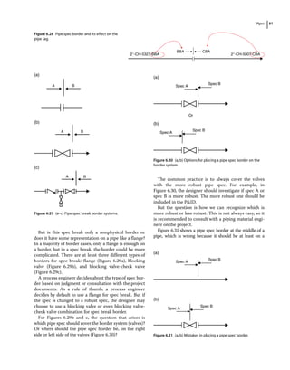
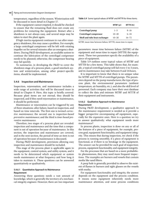
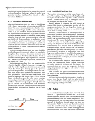
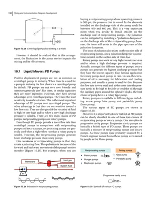
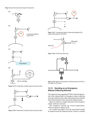
104. Pipes 85
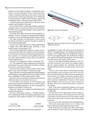
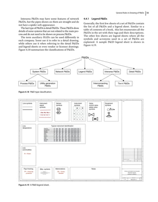
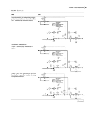
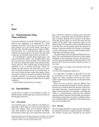
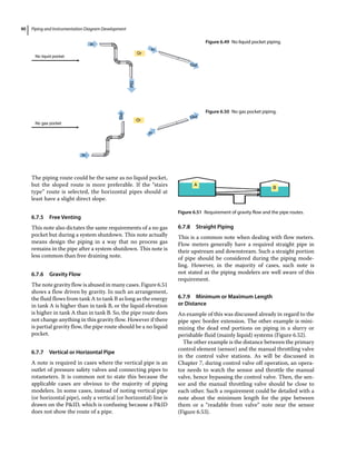
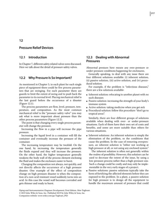
In this arrangement, the first thing to be considered is
making sure that the flow goes in the direction intended.
For all the cases of a single‐source, multiple‐destination
pipe, multiple‐source, single‐destination pipe, and multiple‐
source, multiple‐destination pipe having multiple points
as source or destination is common. For simplicity, only the
cases that have multiple destinations will be discussed.
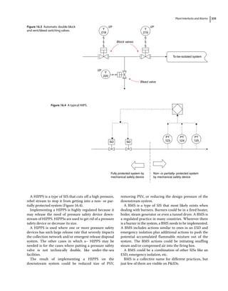
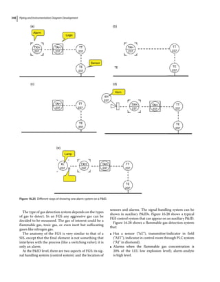
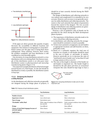
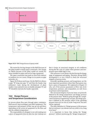
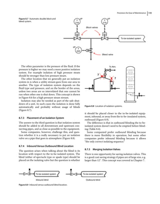
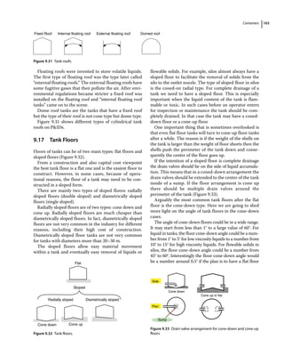
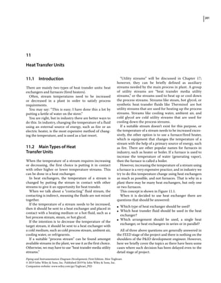
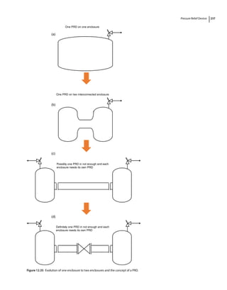
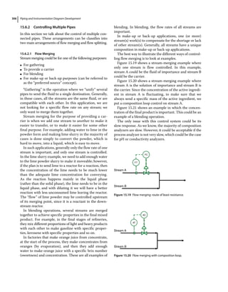
For these cases (as seen in Figure 6.35), the process
requirement could be one of these goals: diverting or
distributing the flow.
In diverting the flow, the goal is to transfer the flow to
only one user at a time, while in distributing the flow, the
goal is to direct the flow with different magnitudes to
multiple users at the same time.
It means that in a multipoint source or destination in
addition to making sure the flow is in the right direction,
secondary goals should also be achieved.
The following sections explain how to satisfy the
requirement of different pipe arrangements.
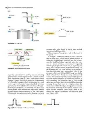
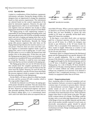
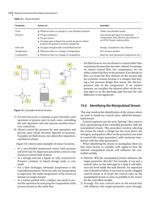
6.6.1 Backflow Prevention Systems [1]
When faced with the issue of reverse flow in pipes, the
process design engineer usually uses a check valve to
prevent the reverse flow. However, using a check valve is
not the best method to prevent reverse flow. There are at
least four different techniques to prevent backflow,
which will be discussed based on their level of effective-
ness in preventing reverse flow.
#1 Air Gap: An air gap is the best way to prevent back-
flow. When an air gap is placed in a flow route there is
absolutely no backflow in the system. However, this
method has some disadvantages. The first is that an air
gap is only applicable for liquid streams; they do not
work on gas streams. The second is that there could be
contamination of the liquid because the stream is
exposed to the environment. Therefore, the environ-
ment should be clean, or the cost of cleaning up the con-
tamination should be factored in. The other downside of
an air gap is that if the weather is cold, there is a chance
of freezing and system failure. However, if somehow all
the disadvantages of an air gap are resolved, it provides
one of the best backflow prevention techniques. An air
gap could be placed in a pipe route or in a tank, and both
are shown in Figure 6.36. It is common to see an air gap
in potable water piping where there is a chance of back-
flow and contamination of portable water with other
contaminated waters.
#5 Backflow‐Preventing Device: Backflow‐preventing
device is a type of device that can be used in clean ser-
vices and is common in water streams. In the casing of a
backflow preventing device, there are two check valves in
series and one pressure safety valve between two check
valves in one casing. If a backflow‐preventing device is
used in a PID, it should be tagged as a specialty item
(SP item) (Figure 6.37).
#2 Inverted U: An inverted U is another way to prevent
reverse flow in a pipe. This method also works only on
liquid streams. By creating a specific arrangement in a
pipe, the backflow of a liquid stream can be prevented.
This arrangement is a vertical upside down U. The height
of this inverted U depends on the pressure of liquid flow
when reversing back. Because of that, in some cases in
which reverse flow pressure is high, the height of the
upside down U will be beyond a practical value. In such
cases, an inverted U cannot be used (Figure 6.38).
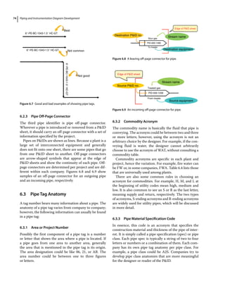
#3 Check Valve: Check valves are the most common
way of preventing backflow. By placing a single check
valve and reverse flow, either a liquid stream or gas
stream will be prevented. However, a check valve always
leaks when trying to prevent backflow. Generally it is
assumed that the conventional swing check valve leaks
about 10% of the flow. The other important parameter
A0
(a)
(b)
(c)
(d)
B0
B1
B0
B0
B0
B1
B2
B2
A0
A0
A1
A1
A2
A2
A0
Figure 6.34 (a–d) Different piping arrangements.
A B
C
D
Figure 6.35 Multiple‐destination pipe arrangement.

105. Piping and Instrumentation Diagram Development
86
regarding a check valve is cracking pressure. Cracking
pressure is the minimum pressure that a stream needs to
have to be able to open up a check valve when a stream
flows in a straight direction. It means that if the pressure
of a flow is low enough, a check valve may not be a good
choice to prevent backflow because the check valve may
prevent even the straight flow. Because check valves gen-
erally leak at backflow, it is commonly said that check
valves prevent liquid backflow, but they cannot prevent
pressure penetration to upstream of the check valve.
This concept is very important when deciding whether a
pressure safety valve should be placed when a check
valve is involved (Figure 6.39).
Different types of check valves will be discussed in
Chapter 7.
#4 Multiple Check Valves: There are some cases that
two or three check valves can be placed in series to
make sure the backflow is prevented and also to mini-
mize the backflow leakage especially when the pres-
sure of a stream is high. A conventional swing check
valve may leak up to 10% of flow rate, so by placing two
swing check valves in series, the backflow leakage can
be decreased only 1%. If the pressure of the stream is
less than 3000 kpag, use a single check valve. If the
pressure is between 3000 and 7000 kpag, use double
check valves. If more than that, a swing of three check
valve is the most appropriate arrangement to prevent
backflow. Some companies go further and indicate in
their guidelines that whenever two or three check
valves are used on a pipe, these should be dissimilar,
meaning if one check valve is swing type, then the
other one should be flow type. This guideline is meant
to maximize reliability of the system because when
there are two dissimilar check valves, there is less
chance that both of check valves will jam at the same
time (Figure 6.40).
Check valve Check valve
PSV
PID symbol
Figure 6.37 Backflow preventing device.
PID symbol
Or
Note: Inverted “U”
Figure 6.38 Inverted U for backflow prevention.
Tank inlet
(a)
(b)
Tank inlet
Air gap
Air gap
Tank outlet
Tank outlet
PID symbol
PID symbol
Note: Air gap
Note: Air gap
Figure 6.36 (a, b) Air gap.

106. Pipes 87
6.6.2 Diversion of Flow
The diverting of flow can easily be done by using several
valves or a few multiway valves. One arrangement can be
seen in Figure 6.41. In this arrangement, diverting valves
work together to send the flow to destination C, B, or D.
Each three‐way valve could be replaced with two con-
ventional (two‐way) blocking valves. The multiway
valves will be discussed in Chapter 7.
6.6.3 Distribution of Flow
The distribution of flow is more difficult. From a purely
theoretical point of view, it can be said that the solution
is manipulating the branches’ diameter and length to get
to the desired flow rate. This solution, however, is not
practical. The length of pipes is generally out of the con-
trol of the process engineer. The designer needs to needs
to follow plant layout, which dictates the pipe lengths.
Therefore, even though this solution may be financially
attractive, it is not practical.
One magic bullet solution is to put control valves on all
branches except one. This solution is shown in
Figure 6.42. However, this solution can be expensive,
especially when large bore pipes (larger than 12″) are
being used.
One branch can always be left without a control valve
because when the flow rates of other branches are regu-
lated by control valves, the flow rate of last branch will be
regulated automatically.
It is important to consider that the branch without a
control valve cannot be the route with maximum resist-
ance. It means that when deciding on the branch without
a control valve, that the branch does not get a minimum
flow because the flow cannot be regulated in a pipe with
constraints.
One alternative solution that only works when the
intention is to distribute the flow evenly is to use sym-
metrical piping. The schematic in Figure 6.43 shows this
solution.
The distribution of flow is not uncommon and
­
wherever there is parallel operating equipment, this
requirement should be met. A note stating, “Symmetrical
Piping,” as in Figure 6.44 shows how this is used.
However, there are still some clients who prefer the
control valve solution for applications like parallel heat
exchangers and who are willing to pay the extra cost
for that.
Placing a control valve to handle the flow distribution
is known as active distribution, and when it is handled
through symmetrical piping, it is known as passive
distribution.
The best symmetrical piping arrangement for a precise
flow distribution is the type in which the main pipe
(before distribution) is perpendicular to the distribution
header. However, in practice there is generally not
enough room to implement such a concept. In practice,
the main pipe could be connected to the distribution
header after a run parallel to the distribution header and
after an elbow. This arrangement generates a deviation
from an evenly distribution goal.
Air coolers are a type of equipment that require good
distribution because of their multiple inlets (and out-
lets). This will be discussed in more detail in Chapter 11.
Figure 6.39 Check valve.
(a)
(b)
Figure 6.40 (a, b) Multiple check valves.
A B
C
D
Figure 6.41 Diverting flow in a multiple‐destination pipe route.
A B
C
D
Figure 6.42 Distributing flow in multiple‐destination pipe route
by control valves.
A
B
D
C
Figure 6.43 Distributing flow in multiple‐destination pipe route
through symmetrical piping.

107. Piping and Instrumentation Diagram Development
88
6.7 ­Pipe Route
Generally speaking, the real pipe route cannot be seen on
the PIDs. There are cases, however, that a special route
should be considered for some routes based on engineering
considerations. Such special pipe routes should be formally
communicated with the Piping group (to develop proper
pipe models and isometric drawings) to make sure they will
be implemented in the plant during construction.
Because this route cannot be shown on the PID, such
special requirements for pipe route should be captured
on the PIDs in the Notes.
A few of these special requirements are sloped, no liq-
uid pocket, no gas pocket, free draining, vertical, hori-
zontal, and minimum length or distance.
6.7.1 Slope
The slope on pipes can be important for horizontal pipes
if a liquid or a two‐phase flows with a liquid component
flowing inside of them. There is no slope for vertical pipes,
and slopes on gas flows are not important. Generally
speaking, horizontal pipes are used without a slope for
different reasons, including the difficulty in handling the
pipe elevation and pipe supports. Therefore, by default
no horizontal pipe will ever have a slope.
There are two features that should be specified on a
pipe symbol: the direction of slope and the slope
magnitude.
The slope direction is the direction of flow (direct
slope) or against the flow (reverse slope). The slope
direction is shown on a pipe with a triangle symbol in
Figure 6.45.
The other feature of a slope is its magnitude. From
theoretical point of view, a slope can be specified by a
percentage, by a fraction, or by the angle. However,
angles (e.g. in degree) are not used to specify slope. A
slope is specified either by a percentage or more practi-
cally by a fraction based on standard lengths of a pipe.
The slope magnitude can be specified on the slope sym-
bol on the PID as 0.5% or 2/12. Here, 12 feet is the
standard length of pipes (Figure 6.46).
Level signal
From LT-1159
From wash water tank
To wash water tank
PID-300-1001
Min. flow
PID-300-1001
To wash water pre-heater
Wash water
PID-300-1003
Wash water Symmetric piping
Seal flush plan 21
WAT-AA-8″-3015
3/4″ 3/4″
2″
1″
1″
1″
1″
1″
3/4″
M M
3/4″
1″
1″
1″
1″ 1″
6×4
6×4
6×4
300-P-130 300-P-140
8×6 8×6
6×4
TSS TSS
3″
4×3 4×3
FO
FC
IS OS
FC
130
FV
130
LC
131
LV
131
FE
130
FE
140
PG
130
PG
141
PG
140
PG
131
WAT-AA-4″-3014
WAT
-
AA
-
4″
-
3017
WAT
-
AA
-
6″
-
3018
WAT
-
AA
-
6″
-
3016
WAT
-
AA
-
8″
-
3016
PID-300-1001
Figure 6.44 An example of symmetrical piping.
Figure 6.45 Slope symbol on pipes.
0.2%
Figure 6.46 Slope symbol and slope magnitude on pipe.

108. Pipes 89
The direction of the slope can be decided during PID
development, but slope magnitude should be calculated
during the design.
The goal of sloping a pipe is to prevent stagnant liquid.
In making a decision on the slope direction, the general
rule is to put the slope toward the more tolerant resource.
For example, in Figure 6.47a, there is a need to slope
the pipe in the outlet of pressure safety valves in liquid
services or two‐phase services (potentially or actually).
In the majority of cases, the outlet flange of pressure
safety valves dictates the horizontal pipe, and also the
flow through the pressure safety valves are not continu-
ous (the pressure safety valves will be opened during
emergencies). Therefore, the outlet pipe should be
sloped. It is not wise to have the remaining liquid stay at
the outlet of the pressure safety valve, because the accu-
mulated liquid at the outlet of pressure safety valve
impacts its operation (refer to Chapter 12 for more
details). Therefore, the slope of this pipe should be away
of the pressure safety valve outlet.
Similar logic is used to put slope on a horizontal pipe,
that is, normally no flow (NNF). This pipe goes to a ves-
sel that is considered a more tolerant system for contain-
ing liquid; therefore, the slope is toward the vessel.
Another example is in steam piping. In steam distribu-
tion networks, there is always a chance of generating
condensation in the pipe. Therefore, steam traps are
installed at specific intervals to remove condensation
from the steam flow, and the pipe is sloped toward each
steam trap (Figure 6.48).
The concept of a steam trap will be discussed later in
this chapter.
The last example is the pipe that directs released fluid
from a pressure safety valve to a collection flare header
(discussed more in Chapter 12). After collecting the
release from different safety devices, the flare headers
direct the liquid to the knockout drum before going to
the flare. As the liquid knockout drum is placed to cap-
ture the liquid from the release gas, it is more tolerant to
liquid and the main header is generally sloped toward the
liquid knockout drum.
If the slope calculation is missed during the design
phase of project, the process engineer responsible for
PID development may decide to put a slope magnitude
on pipes with triangles on them based on rule of thumbs.
The minimum practical slope is about 0.08%, but the
slope of the pipes can go up to 5%. The typical range of a
slope is 0.5% and the typical range is between 0.2 to 1.0%.
For hard‐to‐move or high‐viscosity liquids, 2–3% is not
rare. Underground pipes tend to be at the lower side at
0.2–0.5%. The reason is that if the slope of underground
pipe is a large value, the pipe will be in deep ground at the
destination point. Choosing a lower slope value is more
important when the pipe is long or the underground
water level is high (like near lakes).
6.7.2 No Liquid Pocket
A pipe fully carrying a liquid flow with the chance of
excursion of gas or vapor can be a candidate for no liquid
pocket, means “design in a way that liquid pockets natu-
rally flow and exit the pipe route during the routine
operation of the system”. This phrase directs the pipe
modeler to design a pipe route wherein the gas flow
­
cannot trap a pocket of liquid anywhere in the pipe route
(Figure 6.49). To respond to this requirement, a piping
modeler specifies a pipe route that is vertically down-
ward or has a direct slope.
6.7.3 No Gas Pocket
A pipe fully carrying a gas or vapor flow with the chance
of generation of liquid can be considered no gas/vapor
pocket if the intention is to avoid a stagnant gas pocket
in the pipe during the routine operation of the system.
The term no gas/vapor pocket directs the pipe modeler
to design a pipe route that the liquid flow cannot trap a
pocket of gas anywhere in the pipe route (Figure 6.50).
To respond to this requirement, a piping modeler speci-
fies a pipe route that is vertically upward or has a reverse
slope.
6.7.4 Free Draining (Self‐Draining)
This note dictates the same requirements of no liquid
pocket but during a system shutdown. This note
­
actually means to do the piping in a way that no
­
liquid remains in the pipe after a system shutdown.
NNF
(a) (b)
Figure 6.47 (a, b) Two examples of sloped pipe.
T
Steam
Condensate
Figure 6.48 Example of sloped pipe in steam pipe.

109. Piping and Instrumentation Diagram Development
90
The piping route could be the same as no liquid pocket,
but the sloped route is more preferable. If the “stairs
type” route is selected, the horizontal pipes should at
least have a slight direct slope.
6.7.5 Free Venting
This note also dictates the same requirements of a no gas
pocket but during a system shutdown. This note actually
means design the piping in a way that no process gas
remains in the pipe after a system shutdown. This note is
less common than free draining note.
6.7.6 Gravity Flow
The note gravity flow is abused in many cases. Figure 6.51
shows a flow driven by gravity. In such an arrangement,
the fluid flows from tank A to tank B as long as the energy
in tank A is higher than in tank B, or the liquid elevation
is higher in tank A than in tank B. So, the pipe route does
not change anything in this gravity flow. However if there
is partial gravity flow, the pipe route should be a no liquid
pocket.
6.7.7 Vertical or Horizontal Pipe
A note is required in cases where the vertical pipe is an
outlet of pressure safety valves and connecting pipes to
rotameters. It is common not to state this because the
applicable cases are obvious to the majority of piping
modelers. In some cases, instead of noting vertical pipe
(or horizontal pipe), only a vertical (or horizontal) line is
drawn on the PID, which is confusing because a PID
does not show the route of a pipe.
6.7.8 Straight Piping
This is a common note when dealing with flow meters.
Flow meters generally have a required straight pipe in
their upstream and downstream. Such a straight portion
of pipe should be considered during the piping mode-
ling. However, in the majority of cases, such note is
not stated as the piping modelers are well aware of this
requirement.
6.7.9 Minimum or Maximum Length
or Distance
An example of this was discussed already in regard to the
pipe spec border extension. The other example is mini-
mizing the dead end portions on piping in a slurry or
perishable fluid (mainly liquid) systems (Figure 6.52).
The other example is the distance between the primary
control element (sensor) and the manual throttling valve
in the control valve stations. As will be discussed in
Chapter 7, during control valve off operation, an opera-
tor needs to watch the sensor and throttle the manual
valve, hence bypassing the control valve. Then, the sen-
sor and the manual throttling valve should be close to
each other. Such a requirement could be detailed with a
note about the minimum length for the pipe between
them or a “readable from valve” note near the sensor
(Figure 6.53).
No liquid pocket
In
In
Or
Out
Out
Figure 6.49 No liquid pocket piping.
No gas pocket
In
In
Or
Out
Out
Figure 6.50 No gas pocket piping.
A
B
Figure 6.51 Requirement of gravity flow and the pipe routes.

110. Pipes 91
6.7.10 Other Special Pipe Routes
A U‐shape on a PID does not actually represent the
installing of a U‐shaped pipe. If a piece of pipe with spe-
cial routing will be provided by a vendor, the data sheet
will show the details of the pipe. However, if the special
pipe route will be fabricated by Piping staff in field, it
should be mentioned in the PIDs through a note. It is
common to ignore the note and show the real pipe rout-
ing on the PID by relying on the knowledge of the pipe
modeler.
6.8 ­Piping Movement
A piping circuit can be moved slightly during operation
because of different reasons. One cause of a moving pipe
circuit is thermal expansion and the other is equipment
movement.
Because of the high temperature of service fluid or
temperature variation of ambient air, thermal expan-
sion can expand the piping circuit. Such expansion can
lead to breaks in the pipes if there are no provisions to
handle that.
Equipment movement is another reason for pipe
movement. If a piece of equipment connected to a pipe is
moving, then pipe will move. Again, if this pipe move-
ment is not planned for and stopped in time, the pipe will
be break. There are two main types of equipment that
may cause movement: rotary machine vibration and set-
tlement of big footprint equipment.
Equipment like pumps, compressors, and centrifuges
may continuously vibrate. This vibration will transfer to
all connected pipes if it is not mitigated. However, with
today’s technology and placement of equipment on the
skids, the vibration of equipment is rarely a problem.
The well‐known example of a big footprint equipment
are large tanks. Tanks with a large diameter are consid-
ered big footprint equipment. Several years after tank
fabrication, one side of the tank may settle higher or
lower than the other side of the tank. This may lead to a
marginally tilted tank and the connected pipes are dis-
placed and will eventually break. Tanks settle due to the
nonhomogenous nature of the soil and the imperfect
foundation of the tank. Such settlement is not uncom-
mon and can often be seen in buildings throughout the
world. A few years after a new house is built, some cracks
can appear in different locations of the house, and this is
a result of the settlement of the house.
There are two ways that pipe movement can be
mitigated:
1) Shifting movement: By placing expansion loops on a
pipe circuit, the unwelcomed movement of pipe is
transferred to the elbows, which can handle those
movements better than a straight pipe. Expansion
loops could be in the form of horizontal U‐shapes
(Figure 6.54).
2) Isolation of equipment: By isolation of the pipe circuit
from the moving equipment, the movement will not
be transferred to the pipe circuit. Flexible connec-
tions are used to isolate a piece of equipment. Flexible
connections have symbols, and they are shown in
Figure 6.55 and should be tagged as a SP item in the
Normally
closed
Min.
Min.
Figure 6.52 Min. length of a note to eliminate dead end.
FC
Fit
Readable
Figure 6.53 Min. length of a note for control valve stations.
Figure 6.54 Expansion loop in pipes.
Figure 6.55 Flexible connection on a large bore pipe connected
to a tank.

111. Piping and Instrumentation Diagram Development
92
PIDs. For example, some company guidelines ask
for connecting pipes larger than 4 or 6in. through
flexible connections when they are connected to
tanks to absorb the settlement of the tank. Small bore
pipes are waived from this guideline because they can
handle a few tank settlement by creating a sagging in
the pipe.
Figure 6.56 shows a flexible connection on the inlet of
a centrifugal compressor, although it is not common
these days.
Flexible connections used to have a bad reputation
regarding leakage. But now there are better flexible joints
in the market.
6.9 ­Dealing with Unwanted
Two‐Phase Flow in Pipes
The design and implementation of systems in two‐phase
flows are more difficult than single‐flow pipes. There
are, however, cases in which a two‐phase flow is
inevitable.
When the flow is intended to be a single flow, but then
it turns out to be a two‐phase flow, the piping design is
based on a single phase, and the two‐phase flow should
be eliminated. There are three types of two‐phase flows:
liquid–gas, gas–liquid, and solid–liquid.
6.9.1 Liquid–Gas Two‐Phase Flow
In a liquid–gas two‐phase flow, there is a chance of liquid
droplets in the main stream of gas or vapor. The problem
arises when transferring a gas or vapor because a liquid
can be generated and that is problematic.
Such unwanted two‐phase flows may happen at differ-
ent times. One is when gas comes off of a liquid surface,
like in liquid–gas separators. The other case is when
transferring hot vapors, like steam.
The first step in dealing with this problem is to prevent
the creation of a two‐phase flow. For example, when
transferring a wet gas, heat trace (dashed line beside the
main line) may be used. This solution can be seen in
Figure 6.57.
The next method is to remove the generated liquid
phase from the gas phase as soon as possible before the
creation of a slug of liquids. One example is using a
demister in a gas–liquid separator vessel as shown in
Figure 6.58. For gas streams that come off of a liquid sur-
face, there is always the chance of carrying liquid drop-
lets over into the gas stream.
The other example is using steam trap in steam distri-
bution piping networks. Steam traps remove water con-
densation from the steam (Figure 6.59).
In Figure 6.60, a steam trap is shown as a square with
letter T at the middle. Steam traps should be installed at
predetermined distances on steam transfer pipes, and
the pipes should be sloped toward the stream traps.
Failure to install a condensation removal system in steam
pipes may lead to steam hammering, which may break
the pipes.
There are other symbols can be used on PIDs for
steam traps if the intention is to use the exact type of
steam trap (Figure 6.61).
M
Figure 6.56 Flexible connection on the inlet of centrifugal
compressor.
Figure 6.57 Heat tracing to prevent the generation of
condensation.
Figure 6.58 Demister to prevent carrying over of liquid droplet.
Steam +Condensate Steam trap Steam
Figure 6.59 Stream trap action.

112. Pipes 93
In these applications, steam traps are installed on ver-
tical short pieces of trim pipe known as a steam trap
installation on “drip legs.” Steam traps, however, can be
installed on main pipes. The arrangement of a steam
trap in such an application is more complicated than the
steam trap on a drip leg.
Steam traps need a strainer on the upstream to protect
them from jamming (will be discussed in more detail in
the next section). Drip legs already have a mud column
on their bottom and the steam traps installed on them do
not need a strainer.
They also may need an isolation valve (Chapter 7) for
steam trap inspection, cleaning, or maintenance.
However, adding a bypass pipe loop is always debatable
and will need to be considered fully (Figure 6.62).
In the absence of a steam trap, the isolation valves are
closed and the bypass valve is open, and then the two‐
phase flow bypasses the steam trap and goes down-
stream. It should be ensured that the piping and
equipment in downstream does not damage the pipes or
equipment. In many cases, companies forbid providing a
bypass for steam traps.
Steam traps are a compact version of a two‐phase sep-
arator, which does not need a control system and it only
works on condensate two‐phase streams. This is shown
in Figure 6.63.
Usage of slug catchers can be explained with the same
logic. Slug catchers are a common piece of equipment in
natural gas pipelines. Within the natural gas transfer
through the pipeline, some less volatile components of
the natural gas turn into liquid. Therefore, at some
points, the pipeline may have a two‐phase flow. Although
the natural gas pipeline may be designed to handle the
two‐phase flow of gas–liquid, this not the case for the
equipment downstream of a pipeline. Therefore, there
could be a slug catcher at the end of natural gas pipeline
to remove the liquid portion of the stream from the gas
portion.
The next solution is directing the created liquid phase
to more tolerant system. A liquid phase together with gas
phase is not good for pipes, but the liquid phase can be
redirected to a liquid tank, which is a system that can
handle (and is designed to contain) liquid. In Figure 6.64,
the pipe sloped toward the tank to direct the generated
liquid back to the tank.
The other solution is to ignore it. With this solution
whenever a branch is used from a steam header, the con-
necting point is put on the top of the header to make sure
the generated condensation is not drawn from the header
and the user only receives the steam. The example is
when branches hook up on a flare header or branches
from a bit wet plant air. Generally, the connection point
between the branches of the header is on the top of the
header. Only a note can capture this point on the PID.
In such cases, using some fitting in the pipe route
should be avoided. For example, concentric reducers are
harmful in two‐phase flow streams. The concentric
reducers may change the two‐phase flow from a less
Steam
+Condensate Steam
T
Figure 6.60 Steam trap in steam pipes.
General type T
Thermodynamic type
Inverted bucket type
Figure 6.61 PID symbols for different types of steam traps.
T
NC
? ? ? ?
Figure 6.62 Bypass for steam traps.
Steam+Condensate
T
Condensate
Steam
Figure 6.63 Steam trap function concept.
Figure 6.64 Sloped pipe to direct the liquid phase to more
tolerant system.

113. Piping and Instrumentation Diagram Development
94
­
detrimental regime of dispersed to a more detrimental
regime of slug flow. If placing a reducer is needed on a
potential two‐phase liquid–gas flow, it should be a flat‐
on‐bottom (FOB) one.
6.9.2 Gas–Liquid Two‐Phase Flow
Gas–liquid two‐phase flows may occur in liquid flows
with a chance of generating or ingressing gas bubbles in
them. This issue is much easier to solve than the previ-
ous case because the gas bubbles have a natural ten-
dency to go up. Therefore, they can be removed from
the liquid flow easily. Gas bubbles go up and accumulate
in the corner areas of piping. A gas release system can be
placed in those high point areas to remove the collected
gas bubbles. If the accumulation of gas bubbles is not
very much, the gas release system can be a simple vent
valve. If the accumulation of gas is higher, a gas release
valve or even an automatic time‐driven valve can be
placed. Installing air release valves are common in water
pipes (Figure 6.65).
In these cases, using fittings in the pipe route should be
avoided; for example, concentric reducers are harmful in
two‐phase flow streams. Concentric reducers may
change a two‐phase flow from a less harmful flow to a
more hazardous slug flow. If placing a reducer is needed
on a potential two‐phase gas‐liquid flow, it should be a
flat‐on‐top (FOT) one.
Such unwanted two‐phase flows may happen mainly
when the liquid is cold and is in contact with a gas (or
air). The colder liquid can dissolve more gases, and
when the stream goes through pipes, the pressure
gradually drops and the dissolved gases turn into bub-
bles. Such issue is more problematic in pipelines with
long pipe lengths. One of the cases of gas–liquid flow
could be in suction side pumps when trying to pump a
liquid with dissolved gases. The other case in which an
unwanted gas–liquid flow may be created is when liq-
uid flow with dissolved gases goes through filters or
packed columns. In such situations, each streamline
has a random route; the longer streamlines experience
more pressure drops and the dissolved gas turn into
bubbles.
6.9.3 Solid–Liquid Two‐Phase Flow
The solutions to this issue are similar to gas–liquid solu-
tions. One is getting over the existence of solid phase and
taking the branch from the top of the header, wherever
there is a need for reducer using an FOB type of reducer
on the pipe or making the pipe vertical.
Another solution is removing the solids through a
strainer. This strainer is not a process step, but only for
equipment protection. The bad thing about strainers is
that they are often overlooked, and no one removes and
cleans them when they are full.
Removing a suspended solid by installing a strainer is
unnecessary unless the downstream piece of equipment
has a tight clearances that may plugged and jammed
quickly (e.g. centrifugal pumps, PD pumps, steam traps,
some types of flow meters like turbine flow meters.)
Such unwanted two‐phase flows may happen when
dealing with dirty services. However, the flow during the
commissioning of a process plant is generally dirty.
Commissioning is the first start‐up after the construc-
tion of a plant. Therefore, the fluids in pipes carry debris,
leaves, sandwich wrappers, or used welding rods. Such
large suspended solids can be harmful to the equipment.
Thus, in some cases, even when the flow is clean during
the normal operation of the plant, it could be dirty dur-
ing the commissioning.
The strainers that are placed for the purpose of pro-
tecting the downstream during normal operation
are called permanent strainers, and the strainers for
commissioning are known as temporary strainers.
Temporary strainers are supposed to be removed after
commissioning.
Table 6.7 shows the application of different strainers
for temporary and permanent applications for small and
large bore pipes.
It is important to note that strainers are not installed to
protect items that are already built, but rather to deal
with suspended solids. For example, a strainer upstream
of a slurry pump can be questionable.
6.10 ­Tubes
As was mentioned previously, tubes are pipes with sizes
less than 2″. A general rule of thumb is that a PID lacks
callouts for tubes. However, there are cases where some
tubes may be shown, but they are still not tagged. A well‐
known example is instrument air tubing. Instrument air
generally is distributed through pipes, and they are
shown on the PIDs. However, near the instrument air
users (like control valves), the instrument air pipe is
connected to a manifold that is used as starting point for
several instrument tubes to the instruments. These tubes
Air release valve
Figure 6.65 Air release valve.

114. Pipes 95
are generally not shown unless inside of a control loop
(Figure 6.66).
A “footprint” of tubes may be seen in hot fluid tracers
for piping circuits. When a pipe is steam traced or hot
glycol traced, it can be recognized from the pipe tag or
from a little symbol on the pipe. The symbol generally has
a short line that represents the heat‐tracing tubes. In
other cases, the heat‐tracing tubes may be shown as a
parallel dashed line beside the process pipe. Later, that
dashed line will represent an electrical signal, but this
dashed line representing tracers will not be confused with
the electrical signals because the tracers always are shown
beside the pipes following their routes (Figure 6.67).
The tubing that goes inside of some instruments, like
sensors, is also shown. These narrow tubes are called the
capillary and are shown in Figure 6.68. More information
about this will be provided in Chapter 13.
The other situation that a tube may be used is when
discussing a circular cross section fluid conductors
inside heat transfer equipment. Heat exchanger tubes
and fire‐heated tubes are example of these applications.
6.11 ­Double–Wall Pipes
Double‐wall pipes are available for different reasons.
One application of double‐wall pipes are when jacketing
is needed. For example, in heat jacking, a heating media,
like steam, flows into the annular space, whereas the
main stream flows into the internal pipe of double‐wall
Table 6.7 Applications of different types of strainers for protection.
Pipe size Temporary Permanent
NPS3″ Y‐type strainer T‐type strainer
NPS6″ Cone‐type strainer
Or
Bucket‐type strainer
Instrument air tube
I/P
PC
21
PT
21
PE
21
PY
21
PV
21
Figure 6.66 Instrument air tube inside of control loops.
Tracer (tube conducting hot fluid)
Tracer (tube conducting hot fluid)
Or
Figure 6.67 Fluid heat traced pipe.

115. Piping and Instrumentation Diagram Development
96
pipe. As a rule of thumb, when the temperature differ-
ence between the transferring fluid and the ambient
temperature is more than 100–150°C, insulation is not
effective and heat jacketing (e.g. steam jacketing) should
be used. One example of using double‐wall pipe for this
purpose is transferring molten sulfur.
The other application of double‐wall pipes are when
the intention is to provide a secondary containment
for pipes. Secondary containment will be discussed in
Chapter 9, but in a nutshell, it is an additional enclosing
wall around the process fluid. One example of using
­
double‐wall pipe for this purpose is transferring of toxic
fluids.
The last application mentioned here is using a double‐
wall pipe, whereas the annular space kept under vacuum
works as an insulation layer around the main internal
pipe. This application is more common to provide cold
insulation rather than hot insulation. One example of
using double‐wall pipe for this purpose is cryogenic
ethane. Double‐wall pipes can be tagged separate (each
pipe, inner and outer separately) or within a single tag
(Figure 6.69).
6.12 ­Pipes for Special
Arrangements
Pipes can be placed to provide different features.
6.12.1 Piping for Bypassing
One of the available options when a piece of equipment
isoutofoperationisprovidingabypassforit(Figure6.70).
The bypass pipe could be smaller than the main pipe size
(e.g. one size smaller) because there is no pressure drop
creating an item on it.
The bypass pipe should have at least one blocking
valve on it near its beginning. If the bypass pipe is long or
there is a fear of dead leg, it may need another blocking
valve near its end.
By providing a bypass pipe, the flow automatically goes
through it because the pipe directs the flow to down-
stream, which has a lower pressure. However, if there is
any chance of using the bypass pipe during the normal
operation of the unit, it may need to be equipped with a
check valve to prevent backflow.
Such bypass pipe is needed for closed recirculating sys-
tems (Figure 6.71). This is to give flexibility to the fluid to
the system in recirculating mode or bypassing the unit.
6.12.2 Piping for Recirculation
Recirculation can be needed for different reasons. It may
be part of the normal operation of a unit for recycling
and increasing the efficiency of the unit. Recirculation
may be needed for starting up or cleaning a unit. If recir-
culation is needed during normal operation, the unit
most likely needs to be equipped with a recirculating
pump or a recirculating compressor (Figure 6.72).
6.12.3 Piping for Units in Series
When two (or more) units are in series, the last one gen-
erally works as a trimmer. It is common to see a bypass
LIT
Capillary (narrow tube)
Figure 6.68 Tubes or capillaries for instruments.
Liquid sulfur
From MELTER
5-PID-5.00-1256
S-023-11341-6”x8”-lh-STJ
Figure 6.69 Tagging a double‐wall pipe.
16″
14″
Unit
Figure 6.70 Unit bypass pipe.
16″
16″
14″ Unit
Figure 6.71 Recirculation bypass pipe.

116. Pipes 97
pipe around the trimmer unit. This bypass pipe can be
used during the start‐up of the plant when there is no
real need to bring all the units in operation at once, and
the trimmer unit can be bypassed (Figure 6.73).
6.12.4 Piping for Units in Parallel
Units can be placed in parallel, and their piping is a bit
tricky. Here we want to focus on the pipe sizes in such
arrangement.
It is obvious that if there are two similar equipment in
parallel and one of them is the operating piece of equip-
ment and the other, a spare one (it means 2 × 100%
sparing philosophy), the pipe size does not change after
splitting. This concept is shown in Figure 6.74.
But if both pumps are operating (it means 2×50%
sparing philosophy), the flow splitting on the inlet side of
the pipes in a way that each pump will receive half of the
flow. Here the rule of thumb says that the size of each
branch is 2 of the size of main header, as shown in
Figure 6.75. Based on this, when a pipe flow is branched
to three even flows, the size of each branch would be 3
of the size of main header.
6.12.5 Piping for Pressure Equalization
The pipe for pressure transfer or pressure equalization
can be much smaller than the main pipe size (i.e. two or
three size smaller).
The pipe for pressure equalization can be connected to
two sides of blocking valves for ease of opening or
between two tanks to allow initiating the liquid flow
between them.
6.13 ­
Pipe Size Rule of Thumbs
It is not easy to tell from a PID whether the pipe size
is correct. However, when two or more pipes are con-
nected to each other, it is easier to check the accuracy
of pipe sizing.
Below are some cases through which the pipe size can
be checked:
1) When two (or more) pipes are merging together, the
resultant pipe may have a larger size. Here the word
may is used because there are some cases that this
rule is not valid. For example, when a 2″ pipe is
merged to a 20″ pipe, the size of pipe after connection
of the 2″ pipe is less likely to be changed to a larger
size, like 22″.
2) When a pipe is split into two or more branches, the
size of branches may be smaller than the main pipe.
6.14 ­Pipe Appurtenances
Pipe appurtenances are mainly classified into three
main groups of valves: fittings, process items, and non-
process items.
Valves are piping components that actively affect
flows. Active means they should have a movable part.
A gate valve has a moving stem. A check valve has a
moving flap.
Fittings are piping appurtenances that passively affect
flows. Examples of fittings are elbows and reducers.
Process items are piping appurtenances that are
installed on piping and change some process feature of
the flow. Examples are strainers and silencers. Process
items generally tagged in PIDs as SP item.
Recirculation pump
(b)
(a)
Unit
Unit
Figure 6.72 (a, b) Unit recirculation pipe.
Unit 1 Unit 2
Figure 6.73 Series units pipes.
Unit 1
X″
X″
X″
Unit 2
2×100%
Figure 6.74 Pipe sizes of parallel units, a spare one operating.
Unit 1
X″.(2)0.5
X″.(2)0.5
X″
Unit 2
2×50%
Figure 6.75 Pipe sizes of parallel units, both operating.

117. Piping and Instrumentation Diagram Development
98
Nonprocess items are the items that do nothing to
flowing fluids. Different types of pipe supports and pipe
hangers can be classified in this group. Because they are
not generally shown on the PID, they are not discussed
here. The only nonprocess item that we discuss here is an
insulation joint.
Fittings and special items are discussed in this chapter,
and valves will be discussed in Chapter 7.
6.14.1 Pipe Fittings
Fittings are generally not shown on PIDs except for
four different groups of fittings: reducers and enlargers,
three‐way connections, end‐of‐pipe systems, and pro-
cess flanges. If there should be specific fitting on a pipe
and it cannot be shown on the PID, it can be covered in
the Note area of the PID sheet.
6.14.1.1 Pipe Direction Change
No pipe direction change can be seen on PID. However,
there could be some cases in which the process dictates
using or not using a specific type of pipe direction change
fitting. In such cases, the requirement is put in a note
about the pipe route on the PID.
The most common pipe direction change is a 90‐
degree redirection fitting; however, a 45‐degree fitting is
available, too. A 90‐degree elbow can be standard, short,
or long.
The piping designer always chooses the standard
elbow except in specific cases. When the space is tight, a
short radius rather than standard radius is used. The
long radius is placed only if the PID developer requests
it. The process designer may ask for long radius for spe-
cific cases like slurry piping. The standard radius elbows
are quickly abraded in some slurry piping, and it is wise
to use long radius.
6.14.1.2 Reducers (Enlargers)
The goal in using reducers or enlargers is to increase or
decrease the pipe size (pipe diameter). There are at least
four situations that reducers or enlargers are used.
The first situation is in the case of tying‐in one or more
pipes to another pipe and branching a pipe to more pipes.
In these situations, a reducer or enlarger needs to be used
(depends on the case) to keep the same velocity in the
pipe after adding or deducting fluid flow from the pipe.
If a pipe needs to be branched off to other pipes, it
means that a portion of the flow will be directed from the
main pipe (header) to other pipes, leading to the decrease
in the flow in the main pipe. If the diameter of the pipe is
not decreased, the velocity of fluid in the pipe will be
decreased, which is not a good idea. Therefore, the
reducer is used to adjust the pipe size with the new
reduced flow rate in the main pipe or header. The reducer
should always be placed after pipe branches and not
before them. This can be seen in Figure 6.76a.
In a tying‐in situation, there are one or more pipes that
merge in the main pipe or header. In this situation, the
flow rate of the main header is increased after the addi-
tion of flow through the tying‐in pipes. Again in this
case, an enlarger is used. The important point here is
that the enlarger should be placed before the tying‐in
pipes not after them, as in Figure 6.76b.
The second situation that a reducer or enlarger is used
is when a pipe is connected to a piece of equipment or
instrument. There are some cases that the equipment
flanges do not match the pipe flanges; therefore, a
reducer or enlarger needs to be able to connect pipe to a
piece of equipment, such as connecting suction piping to
a centrifugal pump or connecting discharge piping to the
centrifugal pump. Other examples are piping connec-
tions to inlets or outlet of pressure safety valves and the
pipes upstream or downstream of some control valves.
These examples are shown in Figure 6.77.
We can size a pipe to make sure it matches the equip-
ment or instrument flanges, and by doing this, the
requirement of reducer or enlarger may be waived.
However, this is not always feasible. Equipment and
instruments are sized and manufactured based on the
best equipment or instrument. The sizing criteria for
­
sizing a piece of equipment or instrument are not
(a)
(b)
Figure 6.76 (a, b) Tying‐in and branching‐off piping arrangement.
(a) (b) (c)
Figure 6.77 (a–c) Examples of reducer applications to match the
manufacturers.

118. Pipes 99
­
necessarily the same sizing with those for pipe sizing.
This is why pipe sizes do not always match the equip-
ment or instrument flanges.
The third situation that we need to put enlarger or
reducer is to support specific mechanical strength for a
piece of pipe. For example, if a pipe should go over a pipe
rack, it should be a minimum of 2″ in size, because, as a
rule of thumb, if a pipe is smaller than 2″, it will sag when
it goes over the pipe rack and may need additional support
to prevent this sagging. However, such additional support
is not always available. There are some cases that a process
engineer sizes a pipe and later uses a size less than 2″, for
example, 1 ½″ pipe that goes from point A to point B.
However, if this pipe goes over the pipe rack, an enlarger
may possibly need to be put on the pipe to increase its size
from 1 ½″ to 2″ just before going over the pipe rack. And
after coming down from a pipe rack, a reducer may be
used to change the pipe size back to what the process engi-
neer designed. This example shows a case where both
reducer and enlarger were used to support the specific
mechanical strength of a piece of pipe (Figure 6.78).
The fourth situation is using a reducer or an enlarger
for process purposes. When a pipe is narrower, the veloc-
ity is higher, and vice versa. There are some cases in
which pipes connected to equipment and the pipe is
enlarged before connecting to the equipment possibly to
shorten the fluid jet length inside the equipment if the
long jet disturbs the process inside. In other cases,
enlarging a pipe before connecting it to a tank to reduce
or eliminate the generated electrostatic charge is espe-
cially important when dealing with flammable liquids. If
the inlet nozzle of a tank is narrow, an electrostatic
charge may generated and cause fire.
However, the process engineer is not always neutral
about using reducer or enlarger. Using an enlarger, the
velocity of fluid goes below the acceptable value, making
it unusable. In slurry piping, if the fluid flow velocity
goes below a specific value, sedimentation occurs and
that may lead to the plugging of the pipe.
The symbol for reducers and enlargers are trapezoid.
The sizes of reducers are mentioned below each reducer
or enlarger symbol in a PID. The way the size is shown
is to mention the larger side of reducer or enlarger and a
multiplication sign (×) and the smaller size of the enlarger
or reducer. The examples are shown in Figure 6.79.
However, during the PID development, sometimes a
process engineer asks, What size of reducers or enlargers
are available? Can a reducer be used that reduces the
pipe size from 20″ to 1″? This is best answered by refer-
ring to piping documents; however, it is a good idea
to have a rule of thumb to have some idea about the
available reducer and enlargers. Generally speaking,
the minimum size that a reducer can decrease the size
of a pipe is half of that pipe size. It means with a 20″ pipe,
the reducer, which can be changed more severely, this
pipe size is 20/2 or 10″, which is 20 multiplied to 10
reducers. It means for this case, the available reducers
are: 20×18, 20×16, 20×14, 20×12, and 20×10″.
Reducers and enlargers have two main types: concen-
tric and eccentric (Figure 6.80). Concentric reducers are
less expensive than the more common reducers because
it is a symmetrical piece and fabricating symmetrical
things is cheaper than fabricating nonsymmetrical
things. Therefore, concentric reducers or enlargers are
used unless instructed otherwise.
The difference between concentric and eccentric
reducers is important only in horizontal pipes. When
using eccentric reducers (on horizontal pipes), it should
be cleared if the flat portion is at the bottom or at the top
of the fitting. The position of flat portion of reducers or
enlargers is shown through the symbol or by acronyms of
FOT or FOB near the symbol or both per the company
guidelines (Figure 6.81).
What should be done when the less expensive concen-
tric reducer (or enlarger) cannot be used and the more
expensive eccentric ones have to be used instead?
One main reason is the cost of adjusting pipe supports
for changing the pipe size because of concentric reducer/
enlarger. When/if we use concentric reducer or enlarger,
the pipe supports and hangers should be adjusted
Pipe rack
Figure 6.78 Reducer applications for pipe sturdiness.
4×2 4×2
Figure 6.79 Reducer or enlarger size on PID.
Concentric Eccentric
Figure 6.80 Two types of reducers.
6×4
FOT
10×8
FOB
Figure 6.81 Showing eccentric reducers on PIDs

119. Piping and Instrumentation Diagram Development
100
accordingly. If for whatever reason there is financial con-
straint for designing and also buying different pipe sup-
ports, eccentric reducer or enlarger with FOB can be
used instead (Figure 6.82).
Another reason that may dictate using eccentric
reducer or enlarger is specific for liquid transferring
pipes. An example is facilitating the draining operation
of a pipe circuit. For liquid transferring pipes, the reducer
or enlarger is a conventional concentric is used and full
draining is impossible (Figure 6.83). A reducer or enlarger
that is installed FOB can solve the problem. An example
of this application is for the reducers of control valves
(Figure 6.84).
The full draining is not always important. If the pipe is
a small bore (possibly less than 4″) or the liquid is inno-
cent, it is possible that there is no need to provide full
draining capability such as also in pumping a liquid with
dissolvedgasesasitwasdiscussedpreviously(Figure6.85).
The discharge of the centrifugal pump possibly does
not need the eccentric FOT enlarger because it is most
likely a vertical pipe.
6.14.1.3 Three‐Way Connections
In Section 6.9, a multipoint source and multipoint desti-
nation pipe arrangements are discussed.
When there is a pipe arrangement with multiple
sources or multiple destinations, the concept of tying‐in
and branching off comes to the picture. Both of these
concepts boil down to the question: How is a pipe con-
nected to the middle of another pipe? Generally the
response would be a requirement for a three‐way con-
nection. But there are several types of three‐way connec-
tions. To know which type of three‐way connection
should be used, a PID developer needs to consult the
branch table available in the piping material spec table of
the project. There are different fittings available to do
that including tee’s, reduced‐tee’s, and different types of
O‐lets (e.g. Weldolets, Threadolet).
However, Table 6.8 can be used in deciding on the type
of three‐way connection to be used, and it also shows
the representation of different three‐way connections
on PIDs.
As can be seen from the table, the type of intersection
from PID cannot be figured out. The three‐way con-
nection could be a tee, reduced tee, or O‐let. There is no
specific symbol to recognize a tee from a reduced tee or
from an O‐let. Therefore, a PID will not show whether
a three‐way connection is a tee, reduced tee, or O‐let. If
someone wants to see if the intersection is tee, reduced
tee, or O‐let, the piping spec must be consulted.
6.14.1.4 Pipe Connections
The pipe manufacturers do not fabricate pipes in infinite
lengths. During the construction, the pipes should be
connected to each other, end to end, to make a suitable
length of a pipe route. There are different ways of con-
necting pipes and are shown in Table 6.9. The only type of
pipe connection that is visible on the PID is the flange.
However, flanges are not shown unless there is specific
need for them.
6.14.1.5 End‐of‐Pipe Systems
End‐of‐pipe systems are applied to uncoupled pipes.
Uncoupled pipes are the pipes that are not connected to
other pipes and are not extended.
There are several available options for the end‐of‐pipe
provision listed in Table 6.10. For pipe sizes less than 2″,
a screwed cap or plug can be used. The tendency is
toward using a screwed cap in the newer plants. For pipe
sizes more than 2″, a blind flange or welded cap can be
used. If there is a plan to extend the pipe in the future, a
blind flange is generally used, but a welded cap is enough.
If a frequent connection to other hose is necessary, a
quick connection is the best. Off‐loading systems are
using quick connections because the plan is frequent
transferring of fluid to and from a transportation system.
Figure 6.82 Need for eccentric reducer to use identical pipe
supports.
Figure 6.83 Using FOB eccentric reducer or enlarger to satisfy full
draining of liquid pipes.
Figure 6.84 Using FOB eccentric reducer for control valve.
Figure 6.85 Using FOT eccentric reducer in suction of centrifugal
pump.

120. Pipes 101
Table 6.8 Rule of thumb for selecting three‐way connections.
If
Suitable
three‐way
connection PID representation
Y″
X″
Y is the same size of X Tee
Y is the same is one size
smaller than X
Reduced Tee
Y is smaller than X by two
or three sizes
O‐let
Y smaller than half of X Tee and then
reducer
Table 6.9 Different methods of connecting pipes end to end.
Component Application PID schematic
Socket welding, thread connecting Pipe size less than 2″
Butt welding Pipe size more than 2″
Flange
Table 6.10 Different methods of ending pipes.
Component Application PID schematic
Screwed cap Pipe sizes less than 2″
Plug Pipe sizes less than 2″
Blind flange Pipe sizes more than 2″
Welded cap (with or
without drain valve)
Quick connection Tend to be used in small
to medium bore size pipes
SP

121. Piping and Instrumentation Diagram Development
102
6.14.2 Specialty Items
A plant is a combination of three hardware: equipment,
instruments, and pipes. During the design of plant, the
designers have an opportunity to design the equipment
based on their process requirements. The instruments
are selected based on the control requirement of the
plant by instrument engineers. However, for pipe and
pipe appurtenances, there is no such freedom. The pro-
cess engineer must use whatever size of pipe or other
piping items desired for the plant and put it on the PID.
The Piping group in each engineering company is
responsible for purchasing piping and piping items, and
they generally provide a list of all the acceptable standard
types and sizes of piping and piping items that can be
used in each project. This list is part of a document called
a Piping Material Specification. Basically the Piping
group tells process engineers that only items on the
Piping Material Specification list must be used on a cer-
tain project. However, there are some cases that a pro-
cess engineer or instrument engineer needs a piece of
piping item, and it is not in piping spec. In such cases,
the first option is to try to replace the desired item with
another item in the piping spec. If that does not work,
the Piping group may agree to this as an exception. These
exceptions are considered SP items and definitely cannot
be a long list. Therefore, it could be every non‐equip-
ment item that has not been included in the piping spec.
The Piping group does not care for SP items because
they already know the complete specification of each
item in the piping spec, and it is easy for them to buy the
items from the market. However, for each SP item, the
person who asked for a specific SP item (more than likely
the process engineer) needs to prepare a data sheet for
the item and submit it to the Piping group.
On the PID, a SP item is shown as a little box beside
the item, and the acronym SP with a number, which is
the a tag number (Figure 6.86).
To decide if an element is an SP items, the piping spec
of the project should be consulted. That also means that
there is no universal rule that a non‐slam check valve is a
SP item. However, an experienced engineer may know
that, generally speaking, where there is a check valve in
the project’s piping specs, it is a conventional check
valve, and if non‐slam check valves are required, they are
most likely SP items. When a process engineer includes
an element as an SP item, he/she needs to be aware that
he/she does not have flexibility to choose the sizes
needed as SP items are generally off‐the‐shelf items.
Figure 6.87 shows few examples.
In this figure, a non‐slam check valve, an injection
quill for a chemical injection system, and a flexible
joint are all SP items. In a PID, the designer may
decide to put definition of the SP item beside the
symbol. This is acceptable if the definition is one to
three words in length. Otherwise it is better to not
put the SP item definition on a PID and keep it only
on the SP item data sheet.
Sometimes, there is a dispute between the Mechanical
group and the Piping group if one specific element is SP
item or actually equipment. This is a valid dispute
because if the element is a piece of equipment, it should
be tagged and bought by the Mechanical group, and if it
is an SP item, it should be tagged and bought by the
Piping group. As a rule of thumb, SP items should be
small items on the pipe, meaning elements with less than
0.5m3
in volume without any utility connection and
without any complexity in its structure. If an element is
small but it has a complicated structure, it is better to
classify it as equipment rather than an SP item.
6.14.2.1 Flange‐Insulating Gasket
Here, insulating refers to electrical insulation and not
heat insulation. Galvanic corrosion is arguably the most
common type of corrosion in process plants. Galvanic
or electrochemical corrosion happens when two dis-
similar metals are put in contact with each other.
However, there are some cases that mating flanges are
not similar from material point of view. These situations
happen when there is a spec break in the pipe. The spec
break is almost always on a flange. The flange could be
for pipe, valve, or any other pipe appurtenance. One side
of the flange is from one metallic material, and the other
side is from another metallic material. In such cases, an
electrically nonconductive gasket should be placed
between two mating faces of the flange to prevent elec-
trochemical corrosion. Flange‐insulating gaskets can be
tagged as SP items.
SP
SP
Figure 6.86 Specialty item tags.
SP
SP
SP
Non-slam Injection quill Flex. joint
Figure 6.87 Specialty item examples.

122. Pipes 103
6.15 ­
Other Approach about Piping
In the ordinary approach, pipes are seen as a means of
connecting equipment and containers to each other.
However, the other approach sees pipe circuits in the
background and equipment and other items placed on
the pipe circuits. In this approach, whenever the PID
developer decides to put an item on a pipe, it needs to
be put on at the “best” place. The best place is decided
based on technical and economic measures. Economic
measures direct the PID developer to put the item
wherever is cheaper. Inexpensive options could be a
result of a smaller size item or items in more typical tem-
perature and pressure ranges of operation.
This economical measure may show it is better to
install a valve downstream of a reducer (smaller size) and
not upstream, if the technical measures allows both of
them (Table 6.11). This economic measure may show it
is better to install a flow meter upstream of a centrifugal
compressor (lower pressure) and not downstream, if the
technical measures allows both of them (Table 6.11).
6.16 ­“Merging”Pipes
Pipes are not generally merged. Pipes within process plant
are almost always for a dedicated service. The only impor-
tant exception is by batch, by semi‐batch, and by intermit-
tent operations. In such operations, one single pipe route
may be used for more than one service. For example, in
sand filters, there could be a piece of pipe that during nor-
mal operations carries the dirty water, and during the back
wash, the same piece of pipe carries backwash water.
For a pipeline, it is another story. In pipelines, it is
common to see merged pipes, meaning a single pipeline
may be used to carry different fluids in different time
slots rather than having a dedicated pipeline for each
single fluid. The high cost of developing pipelines justi-
fies using it as shared resource. The important thing
when using a pipe or pipeline as a shared facility is the
cleaning after each use. Without cleaning, there is a
chance of contamination of transferring fluids in pipes
or pipelines.
6.17 ­Wrapping–Up: Addressing
Requirements of Pipe during
the Life Span
In this section, the design is checked to make sure all the
needs of pipes during each phases of plant life are func-
tional. As it was discussed, these phases are: normal
operation, non‐normal operation, inspection or mainte-
nance, and operation in the absence of one item.
1) Normal operation of pipe: The required considera-
tions are already covered.
2) Nonroutine operation (reduced capacity operation,
start‐up operation, upset operation, planned shut-
down, emergency shutdown): This phase of the plant
needs two components to be handled – process and
control and instrumentation. The process component
is discussed here, but the control and instrumentation
component will be discussed in Chapters 13–15.
Generally speaking, pipes do not need to be consid-
ered much during the PID development to cover
nonroutine operations. Pipes are robust items that
can handle different conditions easily.
3) Inspection and maintenance: General consideration
regarding inspection and maintenance of all items
will be covered in Chapter 8. Here, however, we cover
the specific requirements.
4) Pipe are robust items and do not need much attention
during the operation.
Table 6.11 Finding better items for replacing other items.
Better choice Worse choice
Deciding to put an element upstream or
downstream of a reducer
Deciding to put an element upstream or
downstream of a centrifugal compressor
M
M

123. Piping and Instrumentation Diagram Development
104
5) Running plant in absence of pipe: There is generally no
consideration for the times that a piece of pipe is out of
operation because pipes are less prone to breaking.
When a piece of pipe is out of operation, sometimes a
temporary hose is placed to handle the same work.
6.18 ­
Transferring Bulk Solid Materials
However, transferring solid material is more difficult
than transferring liquids and gases. Because of that, there
are plenty of methods to transfer solids, which is suitable
for a limited range of applications.
Transferring solids is more common in plants whose
raw materials are not liquids. The examples are mineral
processing plants and food processing plants.
In the other plants, solid transferring may be used
if the product is solid or there are materials in solid
form.
The first attempt is to design the plant in a more verti-
cal arrangement to transfer the solid by gravity. That is
why it is not unusual to see a solid processing plant
installed in stacked form or with inclined chutes. A com-
mon example is grain processing facilities. This is the
best solution to minimize the use of or ease the use of
solid‐transferring equipment.
Table 6.12 is a nonexhaustive list of bulk solid material
transfer methods. Because solid materials do not go
through the equipment by themselves, plenty of these
solid‐transferring equipment are used as part of other
equipment, for example, belt conveyor–dryer, screw
conveyor–smasher, etc.
­Reference
1 Stephen J. Emery. “Protecting against backflow in
process lines.” Nov. 28, 1990 Chemical Engineering
Magazine.
Table 6.12 Bulk solid transfer methods.
Bulk solid transfer method Explanation Example
Pneumatic transferring in pipes Transferring small size, nonsticky
solids by air
Transferring gypsum powder
Hydraulic transferring in pipes Transferring small size of solids by air Transferring resin beads in ion exchange
systems with ex situ regeneration
Hydraulic transferring in channels Transferring medium to large size of
solids by air
Transferring trees in rivers, Tomato
transferring in tomato‐processing plant
Screw conveyor Transferring very small size, nonsticky
solids, for flowable solids
Transferring starch
Belt conveyor Transferring solids, not necessarily
nonsticky
Transferring solid sulfur
Bucket elevator Transferring large to very large size of
solids by buckets
Transferring ores

124. 105
Piping and Instrumentation Diagram Development, First Edition. Moe Toghraei.
© 2019 John Wiley Sons, Inc. Published 2019 by John Wiley Sons, Inc.
Companion website: www.wiley.com/go/Toghraei_PID
Valves are a type of pipe appurtenances. Other pipe
appurtenances, fittings, and specialty items were already
discussed in Chapter 6.
7.1 ­Valve Naming
Valves are named based on their action on the service
fluid (e.g. throttling valve, stopping (blocking) valve, or
diverting valve) or based on their operating mechanism
(e.g. motor‐operated, solenoid, or manual valve).
Valves can also be named based on their plug type;
they can be a gate, globe, or butterfly valve. Valves can
also be named based on the valve’s location in the piping
(e.g. foot or root valve) or on its duty in the process (e.g.
shutdown, blowdown, or flow control valve).
7.2 ­Valve Functions
Valves are piping appurtenances that actively affect
flows. Active means the valve has a movable part. For
example, a gate valve has a moving stem, and a check
valve has a moving flap.
Any valve with moving mechanism that does not take
order from the outside of the valve can be categorized as
special valve. Check valves, air release valves, and excess
flow valves are examples of special valves. Special valves
are a large group of valves that have specific function. A
few subgroups of special valves will be discussed at the
end of this chapter. Special valves are diverse, which
makes it difficult to classify them, but other valves can be
easily categorized.
7.3 ­Valve Structure
Valves have two main parts: the operator and the plug
(see Figure 7.1). The valve operator is the part that takes
orders from an external source to act on the fluid flow.
The external orders could be an operator’s hand or a
nonhuman actuator. The valve plug is the part of the
valve whose internal portion is in contact with the
fluid. A valve plug can be built such that the valve is
designed either as a throttling valve, an isolation valve,
or a diverting valve.
The valve operator is connected to the valve plug by a
piece of rod called the stem. The stem can move up and
down or can turn depending on the type of the valve.
It is important not to get confused with plug: a plug
is a part in all valves and a plug valve is a specific type
of valve too.
7.4 ­Classification of Valves
There are at least three ways to classify valves: based on
the action of the service fluid and their functions, based
on the number of ports, and based on the number of
seats.
The function of non‐special valves in processing
industries could be any of the following:
1) Adjusting flow valves
2) Stopping flow valves
Valves that adjust flow are valves that change the
magnitude of flow in the pipes. These valves are called
throttling valves. In these valves the valve plug is respon­
sible for changing the magnitude of flow. In theory the
valve plugs can take infinite position between fully open
and fully closed, and hence valves can be categorized as
either partially closed or partially open valves. The
movement of the stem can change the plug position
manually by an operator or via a remotely operated oper­
ator. These so‐called valve operators will be discussed
later in this chapter.
On the other hand valves that stop flow are valves
whose plug can only remain in fully closed or fully open
position. In both positions the valve allows a stream to
flow. Therefore these valves are called blocking valves.
7
Manual Valves and Automatic Valves

125. Piping and Instrumentation Diagram Development
106
A valve is either throttling or blocking based on the
structure and shape of the valve’s plug. These plugs are
discussed later in this chapter.
When placing a non‐special valve in a system, the first
question is if a throttling or blocking valve should be used.
Since each calls for different types of valves, a wrong
decision may cause internal valve leakage (passing‐by) or
premature failure of the valve. The design process engi­
neer can decide whether the suitable duty of valve is
throttling or blocking for a specific situation.
Furthermore valves can also be classified according to
the number of ports: two‐port or multi‐port valves. The
most common valves are the two‐port valves, which have
only two ports (i.e. one inlet and one outlet). However,
multi‐port valves have more than two ports, possibly
three or four. They also have more than one inlet or
outlet ports. Also they can be called by various names
depending on the function of the valve.
Table 7.1 shows the four types of valves and their ­specific
function. Based on the table a two‐port stopping valve
is called an isolation valve. A two‐port adjusting valve is
called an adjusting valve. A multi‐port stopping valve
is called a diverting valve. A multi‐port adjusting valve is
called an adjusting‐diverting valve. The two‐port valves
are by‐default valves, and although the term “two‐port” is
not stated, it is generally assumed to be two‐port valve.
Diverting valves are valves that divert the flow from
one destination to another. Each diverting valve can be
replaced with two or more blocking valves in a specific
arrangement. Adjusting‐diverting valves are valves that
divert a portion of flow from one destination to another.
Each adjusting‐diverting valve can be replaced with two
or more throttling valves in a specific arrangement.
Multi‐port valves have no advantage over the two‐port
valves except saving space and money. They are not as
robust as two‐port valves. Through the use of multi‐
port valves, a huge cost saving is gained specially if using
remotely operated valves (ROT). The remotely operated
valves will be discussed later, but in a nutshell, they are
actually valve actuators. When it is supposed to use
remotely operated valves, merging few of them together
and using multi‐port valve generates a big saving as the
saving in valve actuators are big.
7.4.1 Valve Plug: Throttling vs. Blocking Valves
Throttling valves can adjust the flow anywhere from 0%
(fully closed valve and no flow) to 100% (fully open valve
and full flow). However, the performance of the majority
of these valves is best when they operate between 20
and 80% of flow.
In contrast, blocking valves allow for full flow or no
flow at all. Although using a blocking valve in a throttling
application is possible, it is detrimental to the valve inter­
nals in the long term. Throttling valves can also be used
for isolation purposes, and although this does not
damage the valve internals, they do not generally provide
a tight shutoff (TSO). Blocking valves can be purchased
as a TSO type. The concept is outlined in Table 7.2.
Table 7.1 Valve action vs. the number of ports.
Conventional
(two‐port) Multi‐port
Stopping flow Blocking valve Diverting valve
Adjusting flow Adjusting valve Adjusting‐diverting valve
Table 7.2 Features of throttling vs. blocking valves.
Throttling Blocking
Application Throttling Stopping (blocking, on/off)
Stem travel: appropriate
positions
0–100% wide (20–80%) Zero OR 100% wide
Passing by? Generally no tight shutoff (Could be) tight shutoff
Example A fully open valve may allow, for example,
45m3
h−1
of flow; then a fully closed valve
creates zero flow
A fully open valve may allow, for example, 45m3
h−1
of flow; a partially closed valve may allow, for example,
30m3
h−1
of flow
Interchangeability? Can also be used in blocking applications Cannot be used in throttling applications
Valve operator
Valve plug
Figure 7.1 Structure of a typical valve.

126. Manual Valves and Automatic Valves 107
A valve could be throttling type or a blocking type
depends on the plug structure. A valve can be named
gate, globe, or butterfly type but each of them belongs to
one the groups of throttling or blocking valves.
Gate valves are the workhorses of the industry as
blocking valves. They have a “gate” that goes up or down
and provides a blocking function. Other blocking valves
are ball valves and plug valves. Ball valves are inherently
blocking valves. These have a ball with a cylindrical hole
that rotates in a room. Plug valves can be considered the
grandfather of ball valves. They are similar to ball valves,
but they have a truncated cone inside instead of a ball.
Globe valves are the type of valve used in the industry
for throttling applications. In globe valves a disk adjusts
the flow that is perpendicular to it. Other types of throt­
tling valves are V‐port ball valves and characterized plug
valves.
By changing the shape of the cylindrical hole to a
V‐port hole, a ball valve can be turned into a throttling
type. Using this trick, an inherently blocking‐type ball
valve can be converted into a throttling valve. By cutting
a “characterized” or “segmented” hole, a new throttling
valve can be created. This can be seen in Figure 7.2.
The same trick, that is, cutting a characterized hole in
the plug of a plug valve, can be used to convert a blocking
plug valve to a throttling plug valve.
If the bore through the sphere is the same size as the
nominal size of the valve, the valve is a full port ball valve.
If the bore is one pipe size smaller than the nominal size,
it is a standard port ball valve.
(3) Butterfly valves have characteristics of both throt­
tling and blocking valves, and they can be used for both
purposes; however, because they have high passing‐by
(internal leakage), they are not recommended for blocking
purposes, especially in high‐pressure streams or danger­
ous fluid service (flammable, toxic, etc.). A butterfly valve
does work better as a control valve when the surface of its
disk is not flat and is carefully contoured. Therefore, con­
toured butterfly valves are excellent as throttling valves.
Table 7.3 outlines a non‐exhaustive list of valves in two
applications in process plants: blocking and throttling.
On the PID each valve has a symbol that defined on
the legend sheet of the PID set. However, the symbols
are different from each other in different companies. A
typical list of valve symbols is shown in Table 7.4.
It is important to know that valve functionality, throt­
tling or blocking, is not a stepwise characteristic; they are
rather fuzzier features, meaning a gate valve is not purely
a blocking valve and a globe valve is not purely throttling
valve. This means that a gate valve has more blocking
characteristics than throttling characteristics and a globe
valve has more throttling than blocking characteristics.
With that in mind, it could be said that conventional
butterfly valves have fairly the same level of blocking and
throttling characteristics. This concept is outlined in
Figure 7.3.
Blocking ball valve Throttling ball valve
(V-port ball valve)
Figure 7.2 Two different plugs in ball valves that make it a
blocking or throttling valve.
Table 7.3 Non‐exhaustive list of valves.
Blocking Throttling
Workhorse Gate valve
(Conventional)
ball valve
Butterfly valve
Globe valve
(Full port) ball Valve
Butterfly valve
V‐port ball valve
Characterized plug valve
Others Plug valve Pinch valve
Needle valve
Diaphragm valve
Table 7.4 Valve symbols on PIDs.
Blocking Symbol Throttling Symbol
Gate valve Globe valve
Ball valve Butterfly valve
Plug valve V‐port ball valve
Butterfly valve Characterized plug
valve
Pinch Valve Needle Valve
Diaphragm valve Ball valve (full port)
Angle valve
Can be used as general valve symbol too.

127. Piping and Instrumentation Diagram Development
108
Throttling Blocking
Butterfly Ball Plug Gate
Globe
needle
Characterized ball
characterized plug
Figure 7.3 Valve spectrum regarding their functionality.
In majority of cases, a blocking valve can be considered
a throttling valve only by limiting its range of operation.
It is generally said that butterfly valves work well as valve
in 30–70% of their range.
7.4.2 Valve Selection
There are plenty of resources to help designers find
the appropriate type of valve. A quick‐and‐dirty outline
to find the most suitable type of valve for a specific
­application follows.
The first step is deciding if the valve should be blocking
or throttling. The process designer decides the type of
valve (blocking or throttling) based on the expected func­
tionality of the valve. Generally speaking, the majority
of manual valves in process plants are blocking types.
If there are manual throttling valves, they are mainly on
non‐primary pipes. The automatic valves (or remotely
operated valves) could be either blocking or throttling
depending on the expected function of the valve.
Figures 7.4 and 7.5 show the rules of thumb for decid­
ing on the plug type of valves based on required size and
the environment.
Generally speaking, a gate valve is used as default
choice for a blocking valve, unless it is for very small
sizes (e.g. 3″) that a ball valve is used because miniature
gate valves are expensive. Plug valves could be used in all
the ranges, but they are not as common as gate or ball
valves.
A globe valve is used for a throttling valve, unless it is for
large sizes (e.g. 4″ or 6″) that a butterfly valve is used
because large globe valves are expensive. In smaller sizes a
specific type of globe valve, a needle valve, is used. When
a high pressure drop is needed (e.g. more than 1000KPa),
a specific type of globe valve, an angle valve, can be used.
Characterized plugs, characterized balls, pinches, and
diaphragm valves can be used in all ranges depending on
service and availability.
Figure 7.5 shows the rule of thumb for deciding on the
plug type of valves based on service fluid. There are a
wide variety of available options when the service fluid is
nonaggressive or “innocent.” Butterfly valves are com­
mon in water services, and plug valves are commonly
used for hydrocarbon gases. There are two cases in
which a specific type of valve should be used: aggressive
fluid (e.g. acids, slurries) and uncontaminated fluids (e.g.
streams intended for human consumption).
The most paramount thing when dealing with aggres­
sive or uncontaminated fluids is that no contact between
valve internals (valve trim) and the service fluid is allowed.
Pinch valves and diaphragm valves are the two types of
valves suitable for aggressive and innocent fluids. In a
pinch valve the service fluid is completely isolated from
the valve internals by directing it through an elastic pipe
inside the valve. The diaphragm valve is similar to a pinch
valve (in this respect), but only partially isolates the
service fluid from the valve internals.
Temperature and pressure are other factors to consider
in making a decision on the plug type of valve. If a valve has
polymeric elements (i.e. diaphragm, pinch, and sleeved
plug valves), it has a temperature limitation on its applica­
tion. Deciding which valve to use is dependent on the valve
operators, which will be discussed later in this chapter.
7.4.3 Multi‐port Valves
Multi‐port valves could be either a blocking or throttling
type. Multi‐port blocking valves are better known as
diverting valves. Throttling‐type multi‐port valves are
also available, but they are less common than blocking‐
type multi‐port valves.
Multi‐port valves are not generally listed in a compa­
ny’s piping spec document. If this is the case, it should
Blocking valves
Ball Gate
Plug
3″
Needle
Globe
Butterfly
Plug Ball
Pinch Diaphragm
3″ 6″
Throttling valves
Figure 7.4 Rule of thumb for valve selection based on
functionality and size.
Innocent fluid Aggressive fluid
Gate Globe Butterfly Ball Plug
Water Hydrocarbon gas
Pinch
diaphragm
To-be-pampered fluid
Figure 7.5 Rule of thumb for valve selection based on
environment.

128. Manual Valves and Automatic Valves 109
be tagged as specialty item on the PID. Three‐ and
four‐port multi‐port valves are the most common types,
and they are generally available in sizes less than 6″ at
affordable prices. Multi‐port valves tend to be used in
cleaner services. Symbols for three‐ and four‐port valves
are indicated in Table 7.5.
The blocking‐type multi‐port valves are generally
plug, ball, or globe types. The plug route of multi‐port
valves is different, which allows them to provide different
diverting functionality. The plug route is defined by the
way how a plug redirects the flow. Three‐port valves are
uniquely designed in L port plug. The L port plug pro­
vides flow diversion in L shape (Table 7.6).
Four‐port valves are made in different plug routes:
straightport, Lport, Tport, anddouble‐Lport(Table7.7).
Table 7.5 PID symbol for three‐way and four‐way valves.
Name Symbol
Three‐way valve
Four‐way valve
Table 7.6 Different types of three‐way valves.
Name Internal Position 1 Position 2
“L” port
Table 7.7 Different types of four‐way valves.
Name Internal Position 1 Position 2 Position 3 Position 4
“Dash” port
“L” port
“T” port
“Double‐L”
port

129. Piping and Instrumentation Diagram Development
110
Generally the plug route of multi‐port valves is not
shown; however, if the multi‐port valve is used in a criti­
cal application, it should be mentioned as a note beside
the valve symbol or in the notes area of the PID. An
example of using four‐port diverting valve is shown in
Figure 7.6.
It is shown in the figure that this arrangement reverses
the flow of cooling water to the heat exchanger. The
operator can reverse the flow every few weeks to reverse
the flow of the tube sides to remove fouling from the
tube internals. Probably using a multi‐port valve in this
application is the best because of the following:
●
● The service fluid (i.e. cooling water) is a non‐dirty
service to clog the valve.
●
● The reverse flow practice initiated every few weeks is
not frequent and does not justify the use of several
valves instead of one multi‐port valve.
The multi‐port valves are available for throttling pur­
poses as well. The throttling‐type multi‐port valves are
generally globe types. Multi‐port throttling valves can be
used for combining (mixing) or diverting purposes
(Figure 7.7). One example of using multi‐port throttling
valves is shown in Figure 7.8. In this application the valve
is used to adjust the flow of two streams that are combin­
ing. This valve can be replaced with two conventional
valves that work in a parallel control system. The parallel
control system will be discussed in Chapter 13. Some
designers may decide to use only one conventional
control valve on the bypass stream. This is acceptable
because between two streams, the bypass stream is the
lower resistance route and more flow goes through it.
Therefore, a single control valve on that stream satisfies
the control goal.
7.4.4 Double‐Seated Valves
In PIDs double‐seated valves can be shown as a spe­
cialty item and may use a special symbol.
In reality double‐seated valves are distinguished from
their respective conventional single‐seated valves because
of their bulkier body. In double‐seated valves the stream
is split into two streams and then goes through a dedi­
cated seat for each stream. The main reason for using
double‐seated valves is to reduce the torque required to
open or close the valve. A double‐seated valve acting as
a control valve needs a smaller pneumatic actuator in
comparison with its respective control valve.
Double‐seated valves, however, have an inherent prob­
lem, which is their passing‐by. Because of the complexity
in manufacturing double‐seated valves, they almost
alwayssufferfrominternalleaksorpassing‐by.Therefore
double‐seated valves rarely produce a TSO.
Double‐seated valves can mainly be used in control
valves on high‐pressure streams when there is not
enough room for a large pneumatic diaphragm (e.g. in
debottleneck projects) as long as internal leaks are not a
problem.
7.5 ­Valve Operators
There are two groups of valve operators: manual and
automatic. Manual valve operators are the valves that can
be field adjusted by an operator, whereas automatic oper­
ators that are installed on ROT are the valves that are
controlled remotely from the control room. Automatic
operators are also known as actuators.
The type of valve operator, either manual or automatic,
totally changes the way it is handled in a process plant.
CWR
CWS
CWR
CWS
Figure 7.6 Application of four‐way blocking valve on cooling
water heat exchanger.
Combining Diverting
Figure 7.7 Throttling three‐way valve.
TC
Combining
Figure 7.8 Application of three‐way throttling valve for heat
exchanger control.

130. Manual Valves and Automatic Valves 111
A manual valve is in the domain of the piping group, and
during the design stage of a project, it is tagged (if it is
supposed to be tagged) and procured by the piping group.
A remotely operated valve is listed, tagged, and tagged
by the IC group. Manual operators can be handwheel,
gear operated, or chain operated. When a manual valve
is chosen, a handwheel type is selected by default. The
gear‐ and chain‐operated valves are used in special cases.
When the valve flange size is large, it is difficult for the
operator to open or close it. Therefore gear‐operated
valves are used in large valve sizes. Generally, a valve
with a rotational stream can go from fully open to fully
closed (or vice versa) after three times of nominal body‐
size rotation of the stem. It means that a 4″ gate valve
needs about 12 rounds of rotation to be in fully closed
position from fully open position. When the valve flange
size is equal or larger than 8″, a gear‐operated valve is
used, whereas for valve flange sizes of 6″ or smaller, the
conventional handwheel valve can be used.
Chain‐operated valves are used if a valve is not
accessible to an operator. When a valve is elevated more
than 2 m, it is said to be inaccessible. The solution is to
install a platform or catwalk or use a chain‐operated
valve. Installing a platform or catwalk (not visible on a
PID) is an expensive solution and is justifiable only if
there are many elevated items (including valves and
other pieces of equipment) that can be accessed by the
catwalk. In other cases, only a chain‐operated valve can
solve the problem of an elevated valve.
It is important to know whether a valve is gear oper­
ated or chain operated; it is most likely be tagged as spe­
cialty item on the PID because the majority of piping
specs list only handwheel manual valves.
Deciding between manual (cheaper) and automatic
(more expensive) valves depends on the type of valve
plug (blocking or throttling) and also on the situation.
For a throttling valve to adjust the flow only once in the
life of the plant, there is not really a need to use a throt­
tling valve, so only a restriction orifice (RO) satisfies the
requirement. An RO is less expensive than a valve and is
basically a donut‐shaped plate installed in a pipe to
restrict the flow. The RO acts as a throttling valve
maintained on a specific valve opening. An RO is tagged
as a specialty item on a PID. If a throttling valve needs
to be operated a few times a month, a manual throttling
valve will probably work best. However, a throttling valve
that needs to be changed to different openings several
times in a day or even several times an hour cannot be
manual type, and an automatic throttling valve or control
valve is used instead. This is shown in Figure 7.9.
There are also cases in which a process plant is an arid
and harsh area and expecting an operator to go the field
and change the valve position even a few times a month
could be unrealistic, and a throttling valve should be used.
Also when dealing with toxic material, the designer may
decide to use an automatic operator for the majority of
valves to minimize operator contact with plant facilities.
For a blocking valve, a valve with a one‐time change in
the life of a plant basically means nothing in the pipe
(if the valve supposed to be open always) or a blinded
pipe (if the valve supposed to be closed always). Therefore,
in a case with no change, a blocking valve should not be
used. If a blocking valve needs to be opened or closed
few times in a month or a year, a manual operator is
enough. However, if a blocking valve needs to be change
in the plug position several times in a day, an automatic
operator may be used. This is shown in Figure 7.10.
Generally speaking, there are more manual blocking
valves in process plants than manual throttling valves.
There are fewer manual throttling valves because opera­
tors are needed to change the flow and relying on operators
is not in the best design of the process. There are more
manual blocking valves not because they can be in process
roles or isolation roles (isolation will be discussed in
depth in Chapter 8). Manual valves are more common in
small plants than medium or large process plants.
7.6 ­Different Types of Actuators
To build an automatic throttling valve (or control valve),
a throttling manual valve should be attached to a mod­
ulating actuator. And to build an automatic isolation
Manual
throttling valve
No. movement
month
No. movement
day
No. movement
hour
More movement
0
RO Automatic
throttling valve
Figure 7.9 Rule of thumb for selection of operators for throttling
valves.
Manual
on/off valve
No. movement
year
No. movement
month
No. movement
day
More movement
0
Manual
on/off valve
(with gear if required)
Switching valve
Figure 7.10 Rule of thumb for selection of operators for blocking
valves.

131. Piping and Instrumentation Diagram Development
112
valve, an isolation valve should be matched with an on–
off actuator.
Automatic throttling valves are called control valves,
and automatic blocking valves are called switching valves
(Figure 7.11). There are different types of automatic
actuators available on the market. Table 7.8 summarizes
their features. It can be seen from Table 7.8 that the
majority of actuators are of the modulating type. The
only actuator that is mainly an on–off type is a solenoid
actuator. However, modulating solenoid actuators are
available but are not common. The most common actua­
tors in process plants are diaphragm actuators.
7.7 ­Basis of Operation
for Automatic Valves
An automatic valve can be triggered by time, event, or
human action. Time can be the basis for the operation of
an automatic valve, but this is not true for throttling
valves. An automatic isolation valve can be controlled
with time, and it means that this valve can be scheduled
opened or closed at specific times and for a specific
duration.
This type of application is common for switching
valves in semi‐continuous or intermittent operations.
For example, in a filtration system, the filter is in normal
service (performs filtration) for 23hours, and then it
needs to be pulled out of operation for backwashing for
half an hour. In this example, multiple switching valves
around the filter vessel are scheduled based on time to
handle the operation.
Event‐based automatic valves are automatic valves that
take orders from a sensor signal. This type is common
for both throttling and isolation valves. All control valves
in control loops are event based. The majority of switch­
ing valves in emergency shutdown system are event
based; this means that if the pressure in a vessel goes
beyond a specific number, a switching valve will be
opened to release the pressure.
The last basis of operation is human action, meaning
the operator is in the control room, not in the field; this
means the valve takes orders from a remote operator. For
throttling valves, a remotely operated valve is referred to
as a hand control valve. For blocking valves, a remotely
operated isolation valve is called a shutoff valve.
Throttling valve + Modulating actuator =Control valve
Blocking valve + On/off actuator =Switching valve
Figure 7.11 Control valve and switching valve.
Table 7.8 Different types of actuators.
Type Driver Acronym Type Symbol Application
Diaphragm
actuator
Instrument air AOV On/off or
modulating
The default choice
Piston
actuator
Instrument air On/off or
modulating
Where the diaphragm type cannot be used
(e.g. the required diaphragm area is too
large)
Hydraulic oil HOV On/off or
modulating
H Where instrument air (IA) is not available or
pipe pressure is high
Motor‐
operated
actuator
Electric motor
and AC
electricity
MOV On/off or
modulating
M Where instrument air (IA) is not available.
For large bore pipe size (e.g. 12″)
Solenoid
actuator
Solenoid and DC
electricity
SOV Almost always
on/off
S Mainly for sizes less than 2″, generally on
instrument air tubes (not common for
process pipes)

132. Manual Valves and Automatic Valves 113
7.8 ­Tagging Automatic Valves
Generally speaking, all ROT should be tagged on PIDs.
Table 7.9 summarizes the methodology for tagging auto­
matic blocking valves and throttling valves.
7.9 ­Tagging Manual Valves
Tagging manual valves is not as common as tagging
automatic valves. Some companies do not tag their
manual valves because they consider manual valves to
be less important than automatic valves. However, in
process plants that produce critical products, such as
nuclear power plants, explosive material plants, and
herbicide production plants, it is common to see tagged
manual valves.
The manual valve tag anatomy is generated on a per‐
company basis, but it generally has an alphabetical acro­
nym and a sequential number.
7.10 ­Valve Positions
When talking about valve positions, there are two differ­
ent positions: regular and fail. Regular position is the
position during normal operations of plant, and the fail
position is the position when losing the driver of
“operator.”
The regular position of a valve is an attribute of block­
ing valves, either manual or automatic. Regular position
refers to whether the valve is fully open during normal
operation of the plant. To show this position, an acro­
nym is placed under the valve on the PID. For example,
NO means normally open When a valve is NO, this
means that during normal operation of the plant, the
valve should be fully open, closing only during plant
maintenance, shutdown, and so on.
The fail position of a valve is an attribute of automatic
valves (either throttling or blocking). It refers to the posi­
tion of the valve when the “driver” of the valve is lost (fail
condition). For example, a control valve (automatic
throttling valve) could be called fail open (FO); this
means that if the instrument air to this valve is lost, then
the valve will go to its open position and stop in that
position. Table 7.10 shows the assigning of the regular
position and failure position to the respective valves as a
clarification to the preceding discussion.
In the next two sections, regular positions and failure
positions will be detailed more fully.
7.10.1 Regular Position of Blocking Valves
and Decision Methodology
Regular positions of blocking valves are classified in
three pairs: normally open/normally closed, locked
open/locked closed, and car seal open/car seal closed.
Each could be used in a condition, but all pairs repre­
sent a valve that has a regular position of being open
or closed.
Deciding on the position of block valves is done by
evaluating three items: safety, equipment protection, and
process smoothness (Table 7.11). If a valve needs to be
opened or closed just to support the process, it can be
specified as normally open (NO) or normally closed
(NC). If the decision for the valve’s regular position is
based on equipment protection, then the valve would be
locked open (LO) or locked closed (LC). If a blocking
valve needs to be closed to protect a plant from a hazard,
it is specified as car seal closed (CSC). If it needs to be
open for safety reasons, then this valve is specified as car
Table 7.10 Regular and failure position of valves.
Throttling Blocking
Manual
NC
Automatic
FC
FC
NC
Table 7.9 Two main types of valves and their tagging.
Blocking Throttling
Name of valve Tag Name of valve Tag
Time Sequence valve KV – –
Event Switching valve XV or UV Control valve FV (flow control valve)
Human operator Shutoff valve XV Hand control valve HCV (hand control valve)

133. Piping and Instrumentation Diagram Development
114
seal open (CSO). As a note, not all companies use these
three elements.
To show the regular position of blocking valves, the
corresponding acronym is stated under the valve symbol.
When a valve is NO, this means that during normal oper­
ation of the plant, the valve should be fully open, closing
only during plant maintenance, shutdown, and so on.
NO or NC is used only if there could be confusion
around whether the valve should be open or closed dur­
ing normal operation of the plant. All blocking valves are
generally considered NO valves, unless NO is stated
under the valve symbol. Instead of putting the acronym
NC or NO under the valve symbols on the PIDs, some
companies use a filled symbol of valve to show it is a NC
valve (rather than an outlined symbol). A good example
of using NC valves for all vent and drain valves is when
the vent and drain valves are closed during the normal
operation of the plant and are used only for start‐up.
Examples of using LO/LC and CSO/CSC will be shown
in future chapters.
7.10.2 Failure Position of Automatic Valves
and Decision Methodology
The fail position for an automatic valve could be fail
open (FO), fail closed (FC), fail last (FL), and fail indeter­
minate (FI) (Figure 7.12).
The acronym FL can be a source of confusion because
some interpret it as fail last and others as fail locked. Fail
last means that after losing power, the valve will stay
wherever it was. If this is the concept, it is better to name
it note it as FI because in reality, a valve that stays in its
last position will drift to the open or closed position
because of fluid pressure. If the meaning of FL is fail last,
then drift open or drift closed should also be specified:
FL/DO or FL/DC; otherwise, it will be interpreted as fail
locked. Control practitioners should be aware of this and
clarify the concept of FL to avoid confusion during the
procurement or design of a plant.
The same three elements used in deciding the position
of blocking valves are used to decide the failure position of
an automatic valve: safety, equipment protection, and
process smoothness. Based on these elements, it will be
decided if an automatic valve should be open (FO), closed
(FC), locked in the last position (FL), or stops but not
locked in the last position (or “last,” FL). For automatic
valves, unlike block valves, the selected acronym (FO, FC,
and FL) does not show if the governing decision was based
on safety, equipment protection, or process smoothness.
It means if an automatic valve should be open, FO is
placed below its symbol, no matter why the decision was
made to keep it open.
To decide the failure position of a valve for safety
­
reasons, the need to minimize the hazard in the plant is
the most important. All valves located on high‐energy
streams should generally be FC. Examples of these
streams are a fuel gas stream going to the burner, hot
glycol, and steam. All valves located on low‐energy
streams should generally be FO. Examples of these
streams are cooling water and nitrogen gas. The intent
when determining the failure position based on safety is
to decrease the energy of the plant by lowering tempera­
ture, lowering pressure, and so on.
Sometimes safety does not dictate the failure posi­
tion of the valve, and in such cases, the designer may
Table 7.11 Regular position of blocking valves.
Only for: Blocking valves; manual or automatic
Concept Position in routine operation of plant
Examples
NO NC
Acronyms
CSO, CSC
LO, LC
NO, NC
Safety
Equipment protection
Process smoothness
FO FC FL
FL/DO FL/DC
FI
Figure 7.12 Failure position of automatic valves.

134. Manual Valves and Automatic Valves 115
decide to arbitrarily pick a failure position, such as FC
or FO (which are cheaper than FL), and assign it to the
automatic valve. However, some clients ask the practi­
tioner to use a second decision tool if safety does not
dictate a failure position. In such cases, the second
decision tool (equipment protection) can be used and
then followed by process smoothness if needed. This
means that if safety does not dictate the failure posi­
tion of the valve, the designer should check what the
best failure position of the valve would be to best
­
protect the equipment.
A good example of deciding where to locate failure
positions based on equipment protection is to make a
control valve on a minimum flow line on a set of centrifu­
gal pumps, all of which are FO. In this case, the decision is
made not based on safety, but to protect the pump.
Whether this valve is FO or FC does not impact the safety
of the plant; however, if it is FC, it will impact the integrity
of the equipment or pump. This means that if the valve is
FC and instrument air is lost, then the ­
minimum flow line
of the pump will be blocked and the pump will not be
protected against low‐flow cases and may be damaged.
Process smoothness is the last decision element if the
first two (safety and equipment protection) cannot deter­
mine the failure position of the valve. Process smoothness
basically recommends the failure position that is the best
for the process and that minimizes the fluctuation magni­
tude and extent when a failure happens.
The concept of valve position is summarized in
Table 7.12. When there is no constraint exerted by safety,
equipment protection, or process smoothness, the fail­
ure position is decided based on economic factors; if FO
and FC valves are the least expensive automatic valves,
then one of them is selected. And sometimes the fail
position is not mentioned in the PID at all.
7.10.3 More Concepts about Failure Position
of Automatic Valves
●
● What Is the Failure in Failure Position Discussion?
As was mentioned previously, failure means losing the
driver. Driver is combination of all energy streams that
direct the valve actuator (and consequently the valve
stem) to a specific position. So, in this context, failure
does not refer to mechanical failures or any type of
jamming.
Table 7.13 shows the different actuators and their drivers.
Table 7.12 Failure position of automatic valves.
Only for: Automatic valves; blocking or throttling
Concept Position when losing “operator”
Examples
FO
FC
Acronyms
FC, FO, FL, FI
Safety
Equipment protection
Process smoothness
Table 7.13 Failure reasons of different actuators.
Type Symbol Actuator driver(s) Failure cause(s)
Diaphragm actuator ●
● Instrument air
●
● DC electricity
●
● Losing instrument air
●
● Losing DC electricity
Piston actuator ●
● Instrument air
●
● DC electricity
●
● Losing instrument air
●
● Losing DC electricity
Motor‐operated actuator
M ●
● AC electricity ●
● Losing AC electricity
Solenoid actuator
S ●
● DC electricity ●
● Losing DC electricity

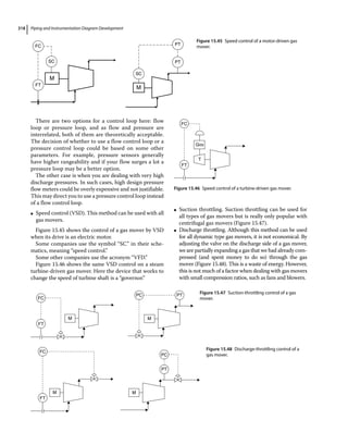
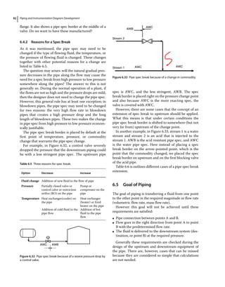
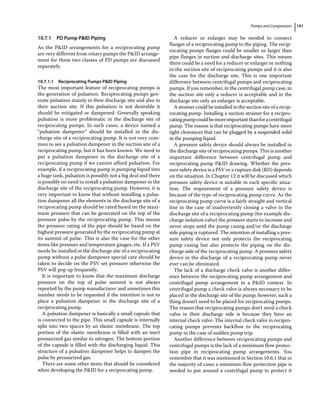
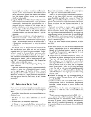
135. Piping and Instrumentation Diagram Development
116
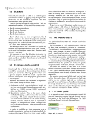
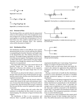
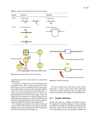
Table 7.15 Automatic valves on PIDs.
Simplistic presentation Detailed presentation
Control valve
FV
FV
P/I
FY
Switching valve
KV
KV
S
Vent
IA
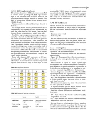
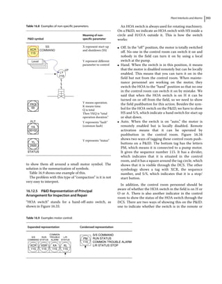
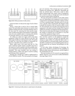
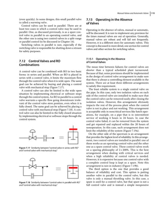
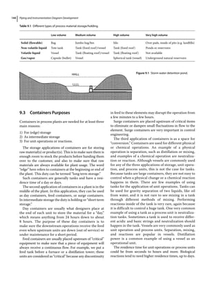
In some types of actuators (i.e. diaphragm and piston
actuators), there are two energy streams as the actuator
driver: instrument air and DC electricity. In these actua­
tors, instrument air moves the main actuator element to
push the valve’s stem. But the instrument air is initiated
to the actuator through one solenoid valve or an arrange­
ment of solenoid valves, which are functioning via DC
electricity. If either of these gets lost, the actuator fails to
function.
Losing instrument air is known as a power loss and
losing DC electricity is known as a signal loss [1].
To what type of failure does the failure position of an
automatic valve refer? Losing instrument air or losing
DC electricity?
If failure position of an automatic valve is mentioned
without any specifics, it is generally because of power
loss. However, to prevent any confusion, it is better to
clearly mention if the failure position is for power loss or
signal loss.
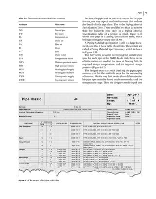
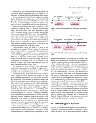
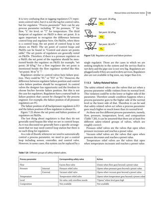
The letter P at the beginning of acronym for failure
position shows it is for power loss, and an S represents
signal loss (Table 7.14).
A process engineer generally wants to have an auto­
matic valve with the same failure position for power
loss and signal loss. Complications can arise if a design
process engineer asks for a failure positions in signal
loss differently than in power loss. The automatic valves
generally report the failure position in cases of power
loss unless another option is needed.
●
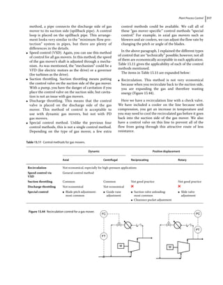
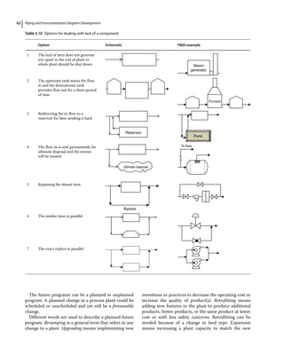
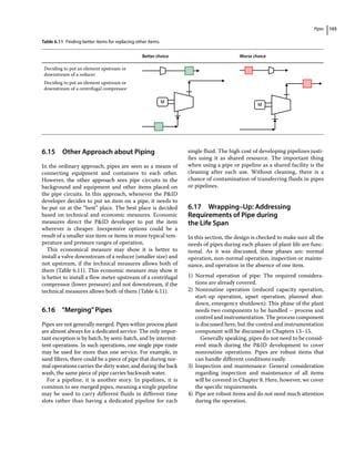
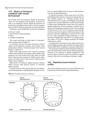
● Actuator Driving System
Showing the driving system of valve actuators on the
PIDs are different for each company. Some decide to
show all the details of the driving mechanism, and others
show only a brief schematic of the system and refer the
reader to other documents for details of the system.
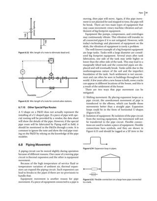
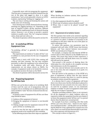
Table 7.15 shows different ways of displaying auto­
matic valves on PIDs in regard to their driver system.
Chapter 13 discusses actuator driving systems in more
detail.
The symbol of a multi‐port valve in the detail of
drivers does not refer to process multi‐port valves.
These valves are common in the hydraulics industry
Table 7.14 Failure case acronyms regarding different types
of driver loss.
Driver loss type Name of drive loss Representing acronyms
Instrument air Power loss PFC, PFO, PFL, PFI
DC electricity Signal loss SFC, SFO, SFL, SFI

136. Manual Valves and Automatic Valves 117
and are known as poppet valves. In the hydraulics
industry, they have specific symbols, but on the PIDs
it is common to use the same symbols for (process)
multi‐port valves for the poppet valves, which could be
confusing. Table 7.16 explains two poppet valves. These
poppet valves are energized by solenoids, so they are a
kind of solenoid valves.
The driving system of switching valves can be compli­
cated depending on the required failure position of the
valve. Manufacturing companies working with different
arrangements of solenoid valves on the instrument air
route and different types of actuators make automatic
valves FO, FC, fail locked, or fail last.
Diaphragm and piston actuators, in this regard, are
single‐acting top spring, single‐acting below spring, and
double‐acting diaphragm/piston. Single‐acting actuators
are the ones whose diaphragm or piston has one instru­
ment air connection and comes with spring. The double‐
acting actuators have two instrument connections and
may not have spring.
Here we do not go any further and just show few
examples in Figure 7.13.
7.11 ­Valve Arrangement
Valves can be installed in single arrangement, in parallel,
or in series.
A single valve can be installed in a piping system with
its flanges attached to nuts and bolts or by welding or
Table 7.16 Explanation of two poppet valves.
Poppet valve name
Symbol
(on PID) Poppet valve structure
3/2‐way valve
Exhaust Piston
IA
4/3‐way valve
Below
piston
Above
piston
IA
Exhaust
FC
3/2-way valve
Fail position: Exhausted
FO
3/2-way valve
Fail position: Exhausted
FL
4/3-way valve
Fail position: Trapped
FO
4/3-way valve
Fail position: Exhausted
Figure 7.13 Few examples showing switching valves with
detailed driver.

137. Piping and Instrumentation Diagram Development
118
screwing its ports by fitting it between the flanges of the
two sides of pipes (Table 7.17).
Generally valves are installed between piping sides
without any other fittings. However, one important
exception is when installing control valves. Sometimes,
the selected control valve has smaller body size that can
be fitted with the pipe size. In such cases, a reducer on
the inlet of a control valve and one enlarger on the outlet
of the control valve may be needed.
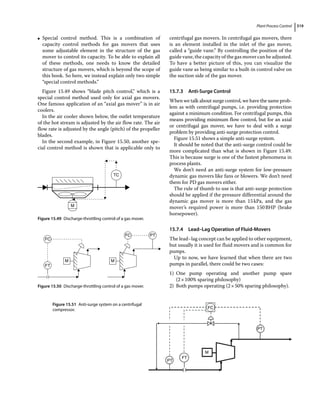
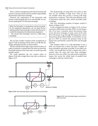
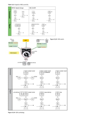
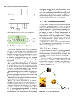
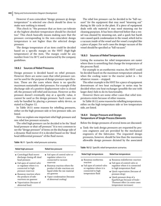
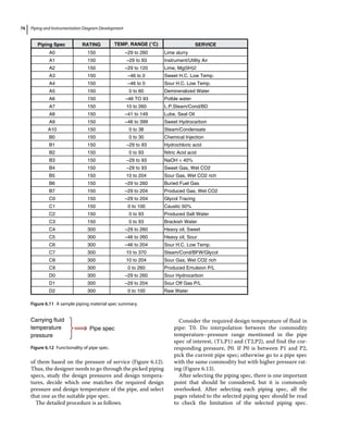
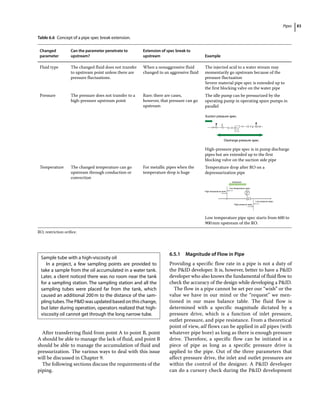
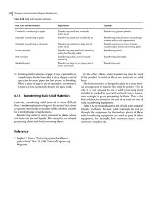
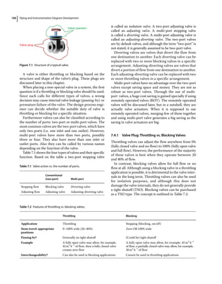
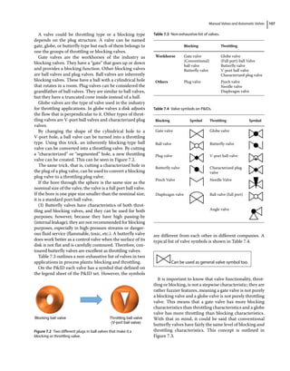
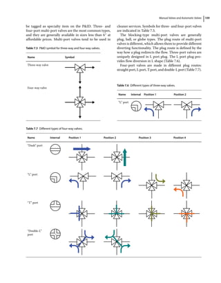
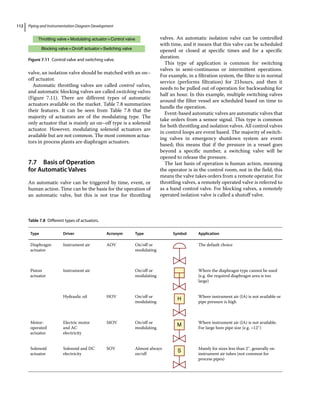
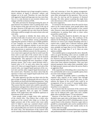
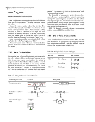
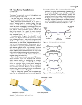
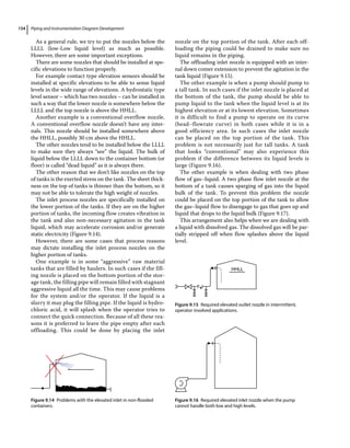
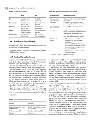
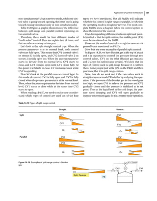
7.11.1 Valves in Series
A manual valve can be used in series, one blocking type
and one throttling type. If a stream needs to be adjusted
manually, and sometimes the stream should be totally
stopped and tight shutoff is important, it is a good idea
to use a manual blocking valve and then manual throt­
tling valve in series (Figure 7.14). This arrangement can
be used in services like toxic fluids or high‐pressure
streams.
Two (or more) manual throttling valves or two (or
more) manual blocking valves are rare, which sometimes
is considered a bad practice in PID development.
However, sometimes having two or more manual block­
ing valves in series happens. Each piece of equipment
needs isolation valves around it for ease of maintenance.
However, when there are two pieces of equipment, one
upstream and one downstream, and they are close to
each other, two of their isolation valves sit close to each
other in a series position. In such cases, one isolation
valve can be eliminated (Figure 7.15).
Valve arrangement in series can be used for control
valves or regulators. These are for the cases that a large
pressure drop is needed in a stream. A large dropping
pressure may cause vibration, noise, and erosion in the
valve [2].
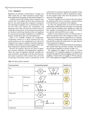
A rule of thumb helps to decide when two regulators in
series may be needed:
●
● Where a pressure drop more than 100psig is needed
(or maximum 150psig).
●
● Where pressure should be dropped to a value less than
1/10th of upstream pressure.
●
● Where the pressure on downstream should be accu­
rately regulated (e.g. less than few psig).
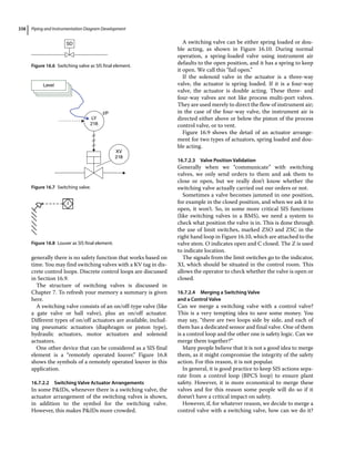
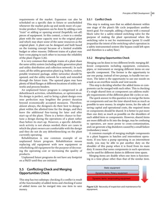
7.11.2 Valves in Parallel
The parallel arrangement of two manual valves may be
used. There are some cases that a manual blocking
valve needs to be placed on a stream that has high pres­
sure. In such cases, placing one single blocking valve,
for example, a gate valve, makes life hard for the opera­
tor who will have to open a manual valve from a fully
closed position under high pressure (e.g. more than
3000 KPa). To solve this problem, another smaller‐
sized manual blocking valve is installed in parallel with
the main valve. When the operator wants to open the
main valve, the small bypass valve is opened at the
beginning to equalize the pressure in both sides of the
main valve, and then the main valve can be easily
opened (Figure 7.16).
Parallel manual valves could be used for other reasons,
such as providing a minimum flow in the pipe even when
the main valve is closed or for start‐up. As was discussed
in Chapter 5, the general method of starting up a piece
of equipment involves gradually opening the valve of the
inlet stream. If the operator does not want to open the
valve suddenly, a parallel and smaller manual valve can
be added to the main valve and the operator can open it
Figure 7.16 Two manual blocking valves in parallel.
Table 7.17 PID symbol for connecting valves.
Valve size Connection type PID sketch
Nominal size 2″ Weld
Screw
Nominal size 2″ Flange
Eq1
Eq1
Eq2
If there are no branches
Eq2
Figure 7.15 Two manual blocking valves in series and saving
opportunity.
Blocking Throttling
Figure 7.14 Manual valves in series: blocking and throttling.

138. Manual Valves and Automatic Valves 119
(even quickly). In some designs, this small parallel valve
is called a warming valve.
Control valves can be used in parallel. There are at
least two cases in which a control valve may be used in
parallel. One, as discussed previously, is as a spare con­
trol valve in parallel to an operating control valve, and
the other one is using two control valves in a split‐range
or parallel control (to be discussed in Chapter 14).
Switching valves in parallel is rare, especially if the
switching valve is responsible for shutting down a stream
for safety purposes.
7.12 ­Control Valves and RO
Combinations
A control valve can be combined with RO in two basic
forms: in series and parallel. When an RO is placed in
series with a control valve, it limits the maximum flow
through the control valve when it is wide open. The same
goal can be achieved by buying and placing a control
valve with mechanical stop (Figure 7.17).
A control valve can also be limited in the wide open
situation by implementing electrical or software stops
through the control system. An RO in parallel to a control
valve warrants a specific flow going downstream irrele­
vant of the control valve stem position, even when it is
fully closed. The same goal can be achieved by placing a
control valve with mechanical stop (Figure 7.18). A con­
trol valve can also be limited in the fully closed situation
by implementing electrical or software stops through the
control system.
7.13 ­Operating in the Absence
of Valves
Operating in the absence of valves, manual or automatic,
will be discussed. It is rare to implement any provision for
the times manual valves are out of operation. Generally,
manual valves are robust and will fail not frequently.
However, it is a different story for automatic valves. This
concept is discussed in more detail, one section for control
valves and other section for switching valves.
7.13.1 Operating in the Absence
of Control Valves
The mean time between failures for control valves are
shorter than a typical scheduled plant turnaround.
Because of that, some provisions should be implemented
in the design of control valve arrangement to make sure
that there is always a controlling element available in the
system. There are at least three different arrangements
to satisfy this requirement.
The least reliable system is a single control valve on
the pipe. In this case, only two isolation valves on each
side of the control valve are installed to make sure that
the control valve can be removed easily after closing the
isolation valves. However, this arrangement obviously
impacts the rest of the process plant when the control
valve is not in place and not working. This arrangement
is acceptable only in noncritical services like batch oper­
ations, for example, on a pipe that is in intermittent
­
service of working 4 hours in 24 hours. In case the
­
control valve failed, it can be removed from the system
and get repaired and replaced within the 20 hours of
nonoperation. In this case, such arrangement does not
limit the reliability of the system (Figure 7.19a).
On the other side of the spectrum is an arrangement
that provides the highest level of reliability. In this arrange­
ment, two control valves are installed in parallel: one of
them works as an operating control valve and the other
one as a spare control valve. These control valves work
on a sparing philosophy of 2×200%. This is the best
arrangement when dealing with critical services and
when a high reliability of control valves is needed.
However, it is expensive because one control valve with
a complete control loop is kept as a spare. Note this
arrangement is rare in industry (Figure 7.19b).
The third option is the one that provides a good
balance of reliability and cost. This option is putting
another valve in parallel to the control valve, but this
valve is only a manual throttling valve. In this case, a
spare is used for a control valve, but that spare is not a
full control valve and is instead a simple inexpensive
Figure 7.17 Similarity between“control valve in series with RO”
and“control valve with mechanical stop.”
Figure 7.18 Similarity between“control valve in parallel with RO”
and“control valve with mechanical stop.”

139. Piping and Instrumentation Diagram Development
120
manual throttling valve. This arrangement is common
for control valves and is called control valve station
(Figure 7.19c).
The basic arrangement of a control station is a control
valve with two isolation valves on each side of control valve,
and the bypass pipe is outside of the isolation valves with a
throttling valve on it (Figure 7.20).
Whenever there is a problem in control valve wherein
the control valve should be pulled out from the operation
and inspected or be sent to the workshop for maintenance,
the isolation valves around the control valve are closed,
and an operator stands up beside the bypass throttling
valve and puts his hand on it while watching the sensor
reading, the sensor that is used to send order to the‐
under‐the‐maintenance control valve and adjust the
opening percentage of the manual valve to mitigate the
system. Here basically we used another control loop in
the absence of the main control loop. However, this fake
control loop is handled by an operator. Definitely an
operator cannot work as a “control loop” for long period
of time because it is very boring and tiring job. However,
it is acceptable to ask an operator to take care of the con­
trol valve duty for short period of time when the main
control valve is under maintenance.
It is obvious that the manual bypass valve is fully closed
in majority of time during the life of a process plant. We
know that throttling valves are not very reliable as a tight
shutoff device. Therefore, in critical services, another
valve could be placed upstream of the bypass valve to
work as a dependable tight shutoff blocking valve. The
example of such critical services could be toxic services,
aggressive chemical services, or high pressure steams.
It will be discussed in Chapter 8 that venting and
draining of the control valve station is important before
performing any inspection or maintenance on it. There­
fore, the operator should fully drain and vent the system.
The important question is how to drain and/or vent this
part of pipe to make sure there is no chance of liquid splash­
ing or gas pushing during inspection and maintenance.
In plenty of cases the control valve flange sizes are
smaller than the pipe sizes. Therefore reducer and
enlarger are needed in the size of the control valve. If the
pipe size is large, it is a good idea to use eccentric reducer
andenlargerinsteadoflessexpensiveconcentricreducer/
enlarger. This trick provides full drainage for the system.
Full drainage of the system is important when the service
is liquid or contained liquid or an aggressive fluid and
Type vs.
Block
valve
Block
valve
Bypass
valve
If tight shutoff
is required
Control
valve
D D
Figure 7.20 Details of control valve station.
Throttling
manual valve
Spare
Operating
2×100%
(a)
(b)
(c)
Figure 7.19 (a–c) Different arrangements for control valves to
provide reliability.

140. Manual Valves and Automatic Valves 121
when the pipe diameter size is large enough to contain a
decent amount of liquid if concentric reducer and
enlarger are to be used. Therefore, for cases that deal
with aggressive liquid and large pipe size (say, more than
3in.), it is a wise decision to use eccentric reducer and
enlarger with flat on bottom (FOB).
The other provision for draining/venting the piece of
pipe between two isolation valves is putting drain valve
on the bottom of the pipe and vent valve on the top of
the pipe. However, if the pipe size is small enough (say,
less than 3in.), possibly just one valve from the bottom
of the pipe could be enough to be used as drain valve and
vent valve.
Now the question is whether the drain valves are
needed in both sides of control valve or just one side of
that. There is a heated debate among professionals
regarding this question. If there is an available guideline
in your company you need to follow, otherwise you
need to make the judgment whether to put two drain
valves in one side of the control valve or just one drain
valve downstream or upstream of control valve. There
are at least three different answers for this question. A
very conservative approach says that we need to put the
drain valve in each side of the control valve to make
sure that each side of the control valve can be drained
independently. This approach is the best for critical
cases like when dealing with toxic, hazardous, or high‐
pressure stream. This is also a good decision when a
control valve is FC. In such cases where the control
valve is FC, there are trapped liquids in each side of the
control valve, one trapped liquid upstream of the con­
trol valve and the other trapped liquid downstream of
the control valve. Therefore, two drain valves help the
operator to drain each trapped liquid easily from each
side of the control valve.
The other approach says that one drain valve for this
piece of pipe is enough. Professionals who are in favor of
this solution are faced with the following question: “what
if the control valve failed or jammed in closed position?”
They answer that the control valve could be opened by a
jackhammer and again there will not be any two separate
trapped liquid. Therefore one drain valve is enough. If we
chose this approach, there are again two available
options: if the single drain valve should be upstream or
downstream of the control valve.
Some people prefer a single drain valve upstream
of the control valve. They believe that a drain valve
upstream of the control valve helps us to drain the
higher pressure side of the control valve more safely
and if it failed to open up a jammed closed control
valve, the other side of the control valve has lower pres­
sure and possibly does not need to be drained through
the drain valve. The downstream of the control valve
can be naturally drained after disassembling the control
valve and removing it from the piping arrangement.
Putting drain valve upstream of the control valve has
some other advantages for the operators. They can use
this valve for start‐up and for purposes of chemical
cleaning. The other option is putting the single drain
valve downstream of the control valve. This option also
has some supporters.
To summarize the discussion about the need for drain
valves on the control station, some people believe that
we need to consider the failed position of the control
valve. However, some other people do not take this into
consideration on putting drain valve or drain valves
around the control valve.
The last thing that should be decided is the type of
bypass manual throttling valve. The workhorse of the
industry for throttling valve is the globe valve. Therefore,
wherever we want to put a bypass throttling valve for a
control valve, a globe valve is selected. However, globe
valves are not available (or are very expensive) in larger
sizes, probably not larger than 4 or 6in. Where the con­
trol valve size is larger than 4″ or 6″, there are some
options available.
One available option is using butterfly valves. Butterfly
valves are good throttling valves and are available and
affordable for large sizes, for example, more than 4 or
6in. However, not all companies and professionals are in
favor of using butterfly valves. The conventional butterfly
valves have some inherent drawbacks. They may have
internal passing‐by that makes them unsuitable valves
for high‐pressure systems and where the service fluid is
an aggressive fluid.
If the required size of throttling valve is more than 4 or
6in. and butterfly valve is not an acceptable option, there
are some exotic designs available.
One completely acceptable option is providing the
required valve capacity of the control valve through
several small (less than 4 or 6in.) globe valves. In this
solution the bypass of the control valve could be an
arrangement of two (or more) 4″ manual globe valves.
This arrangement – shown in Figure 7.21 – is fully func­
tional but is very expensive.
If it is known that the movement of the control valve
stem is only in a short and limited span, a manual globe
valve can be replaced with a gate valve and a smaller
globe valve in parallel (Figure 7.21 top schematic).
However, it has been seen in cases that a company
decided to put a gate valve as the bypass valve for a con­
trol valve. As gate valve is NOT a throttling valve, it is not
a good choice in this situation. However, a gate valve in
parallel to a manual globe valve can be considered if it is
discovered that the control valve mainly works on its
extreme sides of it range.
At the end it should be mentioned that some companies
and professionals believe it is not a good idea to provide

141. Piping and Instrumentation Diagram Development
122
bypass valve for control valves in pressure control loop.
Their logic is that essentially it is very difficult for an
operator to adjust the pressure by a manual throttling
valve. This is especially true when the system down­
stream of the control valve is designed based a lower
pressure and we expect the operator to not only adjust
the pressure but also to take care of the integrity of the
downstream pressure!
Sometimes (and not always) a control valve decreases
the pressure of the fluid severely such that the pressure
of fluid on the downstream side of the control valve is
very low. In such cases, it is a good idea to use less strong
pipe spec on the downstream of the control valve. If the
control valve decreases the pressure a lot and it is decided
to change the spec of the pipe, spec break is needed on
the control station. In such cases the spec break border
should be placed on the downstream of the bypass valve
and downstream of the isolation valve.
However, there could be less common cases that the
condition on the downstream of the control valve is
more aggressive even though the pressure is lower. For
example, there could be an injected acid on the down­
stream. In such cases, based on the rule that says “the
valves internals should be covered by the more severe
piping material spec.,” the downstream piping material
spec. should cover all the valves.
These two arrangements are shown in Figure 7.22.
7.13.2 Operating in the Absence
of Switching Valves
We do not always see “switching valve station” similar to
what we generally see in control valves as “control valve
station.” There are some reasons for that. If a switching
valve is functioning as a shutoff valve, it is very important
for the valve to be closed and to stop flow when needed.
A switching valve with a bypass manual valve provides
the chance that the fluid still flows through the inadvert­
ently left open bypass valve when it is supposed to be
closed. That is the reason why companies are very cau­
tious about implementing “switching valve station.”
However, if it is decided to implement a switching
valve station, it would be similar to the one shown in
Figure 7.23.
The main difference between control valve station and
switching valve station is that in the latter, the bypass
valve should be a blocking valve (and not a throttling
valve).
7.14 ­
Valves in Role of Unit Operation
Throttling valves create shear on the stream flowing
through them. This means throttling valve could be used
as energy injector to the streams. The PID representation
Block
valve
Block
valve
Bypass
valve
Blocking valve
Switching
valve
D D
Figure 7.23 Details of a switching valve station.
Figure 7.21 Options for dealing with requirement of large manual
throttling valve.
Spec. A: severe spec.
Spec. B: severe spec.
Spec. A Spec. B
Spec. A Spec. B
Figure 7.22 Spec. break on control valve station.

142. Manual Valves and Automatic Valves 123
of valve in the role of unit operation can be seen in
Figure 7.24.
In this role the amount of exerted shear in a function
of closeness of valve or the pressure difference that it
creates. Therefore a pressure differential indicator is
required. In the more critical applications the manual
valve could be replaced with a control valve, which could
be connected to a process parameter. Such arrangement
can be used for mixing (or a mixing valve), emulsifying,
or viscosity breaking or other applications.
7.15 ­Special Valves
A valve that does not take any order from an external
independent source is called special valve. A large effort in
the valve industry has been made to develop new special
valves for various applications. As “external independent
source” (e.g. instrument air) is not always available, using
special valves is very beneficial. Such lack of resources
exists in remote areas as well as in small facilities.
In this section we will cover check valves, regulators,
and safety‐related valves.
A check valve is the first special valve to discuss as it
is arguably the most common special valve. The appli­
cations of check valves were discussed before in
Chapter 6.
Regulators are the other group of special valves. Their
concept will be discussed in more detail in Chapter 13.
7.15.1 Check Valves
Check valves are arguably the most important special
valves. They are also known as “non‐return valves” and
“flow direction assurance valves.”
These valves are the type of valves that do not
receive any orders from an external source: they will
be open or closed based on the desired direction of
flow in process.
These valves also need an internal movable member to
move away in the direction of flow and allow the flow in
one direction and, when/if flow starts to reverse, move
on the flow and prevent the reverse flow. There are
principally three ways to implement a movable member:
hanging, lifting, and flexible‐shaped member. Each of
these three could be designed in different structures, but
the main structures are based on flapper, piston or ball,
or an elastomer. Therefore check valves can principally
be classified in four types: swing type, piston or ball type,
and duck bill type.
Table 7.18 shows the different types of check valves
and their symbols.
Conventional piston and ball check valves should be
installed only in vertical position. However, spring‐
loaded piston check valves and spring‐loaded ball valves
can be installed in every position.
“Silent check valve” or “non‐slam check valve” does
not necessarily refer to any specific valve. It only refers
to a check valve in which the backflow preventer
­
element does not get closed suddenly in reverse flow.
A conventional “slam‐type” check valve prematurely
breaks whenever the check valve is used in systems with
frequent and heavy backflows. Here “heavy” means the
reverse movement of a large volume of fluid. The con­
ventional inexpensive “slam‐type” check valves are con­
ventional swing check valves and conventional lift‐type
check valves. The spring‐loaded float check valves are
generally considered as “non‐slam check valves.” Tilting
disk check valve and dual‐plate check valve are other
types of non‐slam check valve.
Table 7.18 PID symbol for check valves.
Movable part Basic type PID symbol
Hanging type Flapper Swing
Lifting/pushing type Piston Conventional piston
Ball Conventional ball
Flexible‐shaped type Elastomer Duck bill
PDI
Figure 7.24 A valve to shear the fluid.

143. Piping and Instrumentation Diagram Development
124
7.15.2 Regulators
Regulators are basically a control loop in a casing, or in
other words they are “fully mechanical control loops.”
SomeapplicationsofregulatorarediscussedinChapter14.
A typical control loop includes sensor controller and a
control valve. If we gather all these three elements and
put it in one small casing, then a regulator is produced.
The advantage of regulator over a control loop is that it
has less items and requires less maintenance and
inspection and it does not need any external source of
energy like instrument air. As for each process parameter
we can have control loop; therefore there are regulators
for each process parameter. Regulators are available for
pressure, temperature, flow rate, and temperature.
There is no available regulator for composition.
Composition sensors or in more technical term pro­
cessed analyzers are too complicated to be able to be
lumped in one casing as a regulator. Therefore regulators
available in the market are pressure regulator, flow regu­
lator, temperature regulator, and level regulator.
However, for pressure, there are two types of regula­
tors: pressure regulators and backpressure regulators.
These two types of regulators basically resemble two
types of pressure control loop: in the first type the pres­
sure sensor is upstream of the control valve, and in the
second type the pressure sensor is downstream of the
control valve. In a pressure regulator the regulator senses
the downstream pressure, while in backpressure regula­
tor the regulator takes order from the pressure in the
upstream of the regulator.
A pressure regulator has an internal valve that adjusts
the opening of the valve to maintain a specific pressure
in the downstream or upstream of the regulator.
In a flow rate regulator there is an internal valve that
will throttle to adjust the flow in the pipe. It is important
to know that by installing a flow regulator in a pipe, the
flow regulator cannot guarantee that the flow is always
on a specific value and all the way in a pipe.
Inside of a level indicator, there is an internal valve in
which the opening of the valve changes to adjust a spe­
cific perimeter line value for a liquid level in a container.
However, a temperature regulator has an internal valve
that throttles to adjust the temperature in a pipe adjacent
to the temperature regulator.
In PIDs there are at least three footprints of regulators:
their symbol, their tag, and their set point. The symbols
for each type of regulators are shown in Table 7.19.
The regulators are tagged in the format of “Process
parameterCV.” CV represents regulator. It is important to
recognize the difference between tagging control valves and
regulators. Control valves are tagged as “Process parame-
terV,” while regulators are tagged as “Process parameterCV.”
Table 7.19 PID symbol for regulators.
Process parameter Corresponding regulator Regulator tag
Flow
FCV
1001
FCV
467
Pressure Downstream
PCV
401
Upstream
Temperature
TCV
324
TCV
400
Level
LCV
567
Composition Does not exist Does not exist

144. Manual Valves and Automatic Valves 125
It is very confusing that in tagging regulators CV repre­
sents control valve, but it is not the tag for control valve,
but for regulator. “Process parameter” here can be any
process parameter including “P” for pressure, “F” for
flow, “L” for level, or “T” for temperature. The third
footprint of regulator on PID is their set point. It is
again important to recognize the difference between
control loop and regulator here. On PIDs, when there
is a control loop, the set point of control loop is not
shown on PID. The set point of control loops and
PIDs can be found in “Control and alarm set points
table.” The set points of regulators are generally noted
on PIDs. Therefore, if there is a pressure regulator on
a PID, the set point of the regulator should be men­
tioned beside the regulator on PID, for example, “set
point; 20 kPag.” For a flow regulator the set point is
mentioned beside the flow regulator symbol like this:
“set point; 30 m3
h−1
.”
Regulators similar to control valves have failure posi­
tion. They could be “FC” or “FO” or “FL.” However, the
difference between regulator failure position and control
valve failure position should be recognized. In control
valves the designer has opportunity and the freedom to
choose his/her favorite failure position. But this is not
the case for regulators. Regulators have a natural built‐in
failure position that cannot be changed by the process
engineer. For example, the failure positon of all pressure
regulators are FC.
The failure position of all backpressure regulators is FO
and the failure position of flow regulators is always FL.
Figure 7.25 shows the set point and failure position of
regulators on PIDs.
The last thing about regulators is that they do not
generally need bypass like what we see in control loops.
As it was discussed we generally have a specific arrange­
ment that we may need control loop station but there is
no such thing for regulators.
As a rule of thumb, whenever we need to automatically
control a process parameter, we need to put a control
loop including sensor, controller, and control valve.
However, in some cases, this system can be replaced by a
single regulator. Those are the cases in which we are
seeking simplicity in the system and the service fluid is
not dirty and the pipe size is not very big. Regulators are
plugged easily if they are used in dirty services. Regulators
also are not available in big sizes, say, larger than 6in.
7.15.3 Safety‐Related Valves
The safety‐related valves are the valves that act when a
process parameter wildly violates from its normal level.
This violation could be in the lower or higher side of the
parameter. Therefore unsafe condition happens when a
process parameter goes to the higher side of the normal
level or the lower side of that. Therefore it can be said
that safety‐related valves act when a process parameter
goes much higher or much lower than its normal level.
As there are five different process parameters, namely,
flow, pressure, temperature, level, and composition
(Table 7.20), it can be assumed that there are at least five
different safety‐related groups of valves, which are
roughly correct:
Pressure relief valves are the valves that open when
pressure increases and reaches a preset value.
Vacuum relief valves are the valves that open when
pressure decreases and reaches a preset value.
Temperature relief valves are the valves that open
when temperature increases and reaches a preset value.
Table 7.20 Different groups of safety‐related valves.
Process parameter Corresponding safety valve Action
Flow Excess flow valve Closes when flow goes beyond a preset value
Pressure Internal Pressure relief valve Opens when pressure goes beyond a preset value
External Vacuum relief valve Opens when vacuum goes beyond a preset value
Temperature Temperature relief valve Opens when temperature goes beyond a preset value
Level No valve, only overflow nozzle “Opens” when level goes high
Composition Not available Not available
Set point: 20 kPag
FC
Set point: 50 kPag
FO
FL
Set point: 30 m3h–1
Figure 7.25 Regulator set point and failure position.

145. Piping and Instrumentation Diagram Development
126
These valves have a fusible plug that melts and ruptures
in a specific temperature. This plug rupturing opens
the valve.
Excess flow valves are the valves that stop the flow
when the flow exceeds beyond the preset value. These
valves are very common in the LPG industry as a safety
measure. If there is a rupture in the pipe, the flow
suddenly accelerates and goes to a flow rate higher
than the preset value of excess flow valve. A typical
symbol of excess flow valve is shown in Figure 7.26.
Some companies consider conventional check valves
as “safety flow valve” and tag them as “FSV.”
Pressure/vacuum safety valves are very important in
process plants and later will be discussed in more detail
in Chapter 12.
7.16 ­Valve Combinations
Developing new valve combinations is another area in
the valve industry. There are dozens of manufacturers
that invent new valve combinations to satisfy a
requirement in the industry. They combine several
valves together and put them in one casing for the
purpose of lowering the cost and making life easier
for plant operators. Examples of such combinations
are “flow preventer device,” “double block‐and‐bleed
device,” “gate valve with internal bypass valve,” and
“minimum flow device.”
The downside of such devices is their lower redun­
dancy. Because a fairly complicated system is placed in a
casing, they are more prone to failure, and also failure
may impact larger area. For these reasons the large com­
panies that have enough budget generally prefer to buy
individual items and assemble them in the plant rather
than buying combined devices.
Table 7.21 shows few examples of valve combinations
and the proposed PID symbol for them.
7.17 ­
End of Valve Arrangements
There are different ways to “blind” a valve at the end of a
pipe. To find out an appropriate way, the piping material
spec. should be consulted. There are however rules of
thumbs that are mentioned in Table 7.22.
Table 7.22 Arrangements of valves in end of pipes.
Pipe size Joint name PID schematic
NPS2″ Screwed plug
Screwed cap
NPS2″ Blind flange
Figure 7.26 Excess flow valve PID symbol.
Table 7.21 PID symbol of some valve combinations.
Combined system name Schematic PID symbol
Flow preventer device
Double block‐and‐bleed
device
Gate valve with bypass
valve

146. Manual Valves and Automatic Valves 127
If a pipe ends to a valve or quick connecting fitting and
needs to be opened frequently, it may need additional
provisions to protect its environment.
Drip catching system may be needed wherever there is
a non‐coupled valve or quick connection in liquid
services.
With today’s ever‐tightening environmental standards,
the codes for allowable amount of liquid spills have
become tighter and tighter. The liquid spill codes in
different countries limit the amount of spilled liquid in a
specific time period. Such limitation could be different
for different liquids.
If spills are not allowable, a drip catching system should
be installed at non‐coupled valve or quick connection.
Figure 7.27 shows a simple drip catching system.
7.18 ­
Valve Sizing Rule of Thumbs
It is important to know there is difference between valve
body size and valve internal size.
Valve body size represents the size of its flanges or the
size of pipe ends in order for a valve to be fitted to them
without the need of any reducer/enlarger.
Valve internal size is the nominal size of the valve
internal represented in the form of a pipe equivalent size.
Each valve body size may have up to three different
valve internal sizes. What is seen on PID is only the
valve body size. However, if a valve internal size is impor­
tant, it should be covered in the notes area.
The rule of thumb for valve sizing could be split into
two main types of valves: blocking and throttling.
The blocking valves generally have the same size that
of the pipe. For example, a 6″ pipe size needs a gate valve
of 6″, or a 10″ pipe needs a 10″ (gate) switching valve.
However, the case for throttling valves is not that
simple. The size of throttling valves, either manual or
automatic, needs to be specified during the design
stage of the projects.
While this is true, as the manual throttling valves
generally play role in very noncritical situations, the
designers may decide not to do the specified size and
simply pick the same size that of the pipe for the manual
throttling valve. It means that in noncritical service a 8″
pipe may need a 8″ globe valve.
However, this is not case for automatic throttling
valves or control valves. While sizing of the control valve
needs extensive calculation, we can just check the body
size of control valves.
As a rule of thumb, the size of a control valve could be
between minimum half size of the pipe and the same size
of the pipe. The typical control valve size is one size
smaller than the pipe size. It means that for a 10″ pipe, it
is not odd to see a control valve of 6″ (half of 10″) or even
10″, but the control valve size on this pipe is typically 8″
(one size smaller than 10″).
This rule of thumb has exceptions especially for cases
where pipes for some reasons are oversized.
The control valves on small bore pipes (say, less than
4″) are generally the same size of the pipe.
7.19 ­Merging Valves
Valves are not generally merged. In Chapter 6 we dis­
cussed about the cases wherein a pipe can be merged.
Whenever a pipe is merged and handles more than one
duty, all the valves on the pipe, including manual and
automatic ones, are shared as well.
7.20 ­
Wrapping Up: Addressing
Requirements of Valve During
the Life Span
In this portion we check our design to make sure we
cover all the needs of valves during each phase of plant
life. As it was discussed before, these phases are normal
operation, non‐normal operation, inspection/mainte­
nance, and operability in the absence of one item:
1) Normal operation of valves: The required considera­
tions are already covered.
2) Nonroutine operation (reduced capacity operation,
start‐up operation, upset operation, planned shut­
down, emergency shutdown): This phase of plant
life needs two components to be handled: process
component and control/instrumentation compo­
nent. The process component is discussed here,
but the control/instrumentation component will be
discussed in Chapters 13–15.
Generally speaking, valves do not need much con­
sideration during the PID development to cover
nonroutine operations. These valves are very robust
items that can handle different conditions easily.
NC
Figure 7.27 Drip catching system.

147. Piping and Instrumentation Diagram Development
128
On the other side automatic valves need some atten­
tion. We already talked about control valves.
3) Inspection and maintenance: General consideration
regarding inspection and maintenance of all items
will be covered in Chapter 8. Here, however we cover
the specific requirements.
Manual valves are very robust items and do
not need much attention during the operation.
On the other side automatic valves needs some
provisions. We already talked about the required
provisions for control valves and switching valves.
One other inspection for switching valves is
“stroke test,” which does not have any footprint on
PIDs.
4) Running plant in the absence of a valve: This stage
was also covered before.
­References
1 Meier, F.A. and Meier, C.A. (2011). Instrumentation and
Control Systems Documentation, 1e. Research Triangle
Park, NC: International Society of Automation Print.
2 “Two Pressure‐Reducing Valves In Series – Xylem
Applied Water Systems – United States”. Xylem Applied
Water Systems – United States. N.p., 2017. Web. 24 May
2017. http://bellgossett.com/2016/03/28/two‐pressure‐
reducing‐valves‐prvs‐in‐series‐two‐step‐pressure‐
reduction.

148. 129
Piping and Instrumentation Diagram Development, First Edition. Moe Toghraei.
© 2019 John Wiley Sons, Inc. Published 2019 by John Wiley Sons, Inc.
Companion website: www.wiley.com/go/Toghraei_PID
8.1 ­Introduction
PID development for the purpose of inspection and
maintenance was briefly discussed in Chapter 5. This
concept, however, is so important it needs a chapter
devoted to it.
This chapter is about the required provisions that
should be considered in PIDs to facilitate an inspection
and/or maintenance operation.
These provisions are used for the purpose of facilitating
inspection and maintenance, and also sometimes as part
ofashutdownsystem.Theinstrumentationrequirements
of safe shutdown are mentioned in Chapter 15 but here
the process requirements are mentioned.
In this chapter we discuss the requirements of three
elements of each process plant: equipment, utilities
and instruments regarding ease of maintenance and
inspection.
The inspection/maintenance of instruments and util-
ity systems is also mentioned here.
8.2 ­
Different Types of Equipment Care
From a maintenance viewpoint, “equipment care” can be
categorized based on the location of applying care and
the timing of the care.
The care could be done in workshop, or “in‐workshop
care,” or could be done when the piece of equipment is
not dislocated, “in‐place care.”
The in‐place care can be categorized further into
“in‐line” or “off‐line” operation.
The in‐line care is performed during the operation of
the unit of interest while in off‐line care the unit of
interest has to be pulled out of operation for the required
care. We love equipment and units that need in‐line care
rather than off‐line care. One attempt of equipment
fabricators is to develop new equipment with less need
for off‐line care and more in‐line care. For example in
upstream oil extraction there is a piece of equipment
called an FWKO drum or “free water knock out drum.”
This vessel may see heavy settlement of sands in it. In
older days, at specific intervals the FWKO drum would
be taken out of service for “de‐sanding operation” but
these days there is equipment with automatic de‐sanding
systems that can remove the sand from them during the
normal operation of FWKO drums.
Although it could be said that major maintenances
occurs in workshops and only minor repair can be done
in-place but it is not the cases always. There are some
huge equipment that all of their maintenance-small or
big- should be done in field, or “in-place care”. Tanks are
a famous example of them.
Each of these two different types of equipment care
forces us to provide different types of provisions for
equipment on PIDs.
Table 8.1 shows the responsibility of different groups
in process plants for different types of equipment care.
8.3 ­In‐place In‐line Equipment Care
“In‐place in‐line care” means any activity that takes care
of a process item without any disturbance to the normal
operation of the element or with just mild disturbance.
There are mainly two types of activities in this group:
activities related to the rejuvenation of the equipment
and activities related to monitoring the equipment.
Rejuvenation activities are needed for equipment that
is inherently in an intermittent or semi‐continuous mode
of operation. One example of rejuvenation activities has
already been stated as de‐sanding in FWKO drums.
The rejuvenation activities could be triggered by one
or a combination of these parameters. They can be initi-
ated by receiving a specific sensor signal (event based),
or they could be initiated after a specific time interval
(time based), or by the decision of the operator.
From the type of operation viewpoint, a rejuvenation
process can be done manually or automatically. In manual
8
Provisions for Ease of Maintenance

149. Piping and Instrumentation Diagram Development
130
rejuvenation all the operation are performed by
operator(s) in the field. In automatic rejuvenation the
operation can be done fully automatically without any
action by an operator, or can be initiated and observed by
an operator from the control room (and not the field).
Manual rejuvenation is done if the rejuvenation doesn’t
need to be very frequent, or the rejuvenation steps are
not very complicated, or if the unit of interest doesn’t
have very critical role in the plant. Otherwise automatic
rejuvenation should be performed.
Below are a few examples of equipment requiring
rejuvenation activities.
Sand filtering in water treatment operation is generally
a semi‐continuous operation. After a certain time period,
the filter should be taken out of operation for backwash-
ing. This type of operation should be implemented dur-
ing the design and be shown on a PID. The backwashing
could be manual (in small systems) or automatic. The
backwashing operation is a type of “in‐place in‐line care.”
Another example is a soot blower for heating coils in
the convection section of fire heaters and boilers. These
coils get covered with soot after a while. To keep the
same efficiency of the fire heater or boiler this soot
should be removed from them. A soot blower is a moving
set of perforated pipes that slide into the convection
section of fire heaters and, by injecting steam, dislodge
the precipitated coke or soot.
Another example is the cleaning of bin filters. Bin
filters are a type of in situ treatment of bin vents. Bin and
silo vents may have a large amount of dust. To remove
the dust from the outgoing gas (air) a bin filter can be
installed on the vent of bins or silos. It is very common to
use bag filters in the role of bin filter. In each bag filter
there are several filter bags (socks) that separate the dust
from the gas stream. These socks get full after a while
then need to be rejuvenated. The rejuvenation of each
sock can be done by backflowing an air jet in it. As there
are several socks in each bag filter. One sock can be
cleaned during normal operation with marginal impact
on the operation of the bag filter.
The last example of rejuvenation is the regeneration of
ion exchange systems. Ion exchangers in, for example,
water treatment systems don’t work on a fully continuous
basis. They function to adsorb the ions on their “exhaus-
tion period.” At the beginning of this period the resin
beads inside of the ion exchange vessel are fresh and ready
to adsorb ions. After a while the resign beads are “filled”
with ions and become exhausted. To return them back to
their fresh condition, the resin beads should be “regener-
ated.” This regeneration, which is a type of rejuvenation, is
done by sending a solution through the ion exchangers.
A large group of rejuvenation operations are catego-
rized as “cleaning.” The different cleaning methods are
discussed later in this chapter. It is very common to do
automatic rejuvenation. The automatic rejuvenation can
be provided by a mechanical unit that recirculates the
cleaning agent or object. The automatic rejuvenation
systems are any of two main types of “mechanical‐in‐
place” (MIP) systems, or “clean‐in‐place” (CIP) systems.
These systems will be discussed later in this chapter.
Activities related to monitoring equipment in in‐line
care are mainly on the shoulders of the “rounding”
operator. The operator could be equipped (beyond just
personal safety equipment) or non‐equipped. If the
operator is non‐equipped, he/she relies on his/her five
senses. Among them, the taste sense never is used. Below
is a non‐inclusive list of the use of the remaining four
senses of the rounding operator:
●
● Vision: leakage, vibration, overflow of tanks, checking
levels, checking flame color and shape
●
● Hearing: vibration, cavitation, hammering, PSV
release, explosion
●
● Touch: vibration
●
● Smell: fire, leakage, PSV release to atmosphere.
To facilitate the duties of the rounding operator, the
process engineer can put some items on the PID. The
examples are sight glasses to check liquid levels, catalyst
levels, or filtering media levels, and peep holes to check
the color and shape of flames in a furnace or boiler.
An equipped rounding operator can have some small
measuring devices to check some parameters that can-
not be accurately checked without. It could be a portable
pressure gauge, portable temperature sensor, etc. If it is
the plan to have an equipped rounding operator, the pro-
cess engineer needs to provide “test points” on impor-
tant points of the system for him. They could be a
“pressure tap” (PT), or “temperature point” (TP).
However, these points should not be very important
parameters because if one parameter is very important
to check and monitor, it should be part of a control loop.
An example of a PT could be the suction side of centrifu-
gal pumps. In some companies the acronym of PP is used
for “pressure point” and TW for “thermowell.” This con-
cept will be discussed in more detail in Chapter 13.
8.4 ­
In‐place Off‐line Equipment Care
“In‐place off‐line” care could be for small repair jobs,
inspection, or as a preliminary step for “in‐workshop off‐
line care” activities.
Table 8.1 Different types of equipment care.
In‐line Off‐line
In‐place By process group By mechanical group
By mechanical group
In‐workshop Not applicable

150. Provisions for Ease of Maintenance 131
It generally starts with de‐energizing the equipment.
Then the piece of equipment should be isolated from the
rest of the plant and tagged to show it is under
maintenance. Such activity generally is known as LOTO
in plants, representing “locking out–tagging out.”
The next step is venting and draining the system and
finally some sort of cleaning.
Such cleaning may include chemical/solvent cleaning,
steaming‐out, pigging operation, etc. Depending on the
type of required in‐place off‐line operation, different
items should be implemented (such as chemical cleaning
valves). However, a set of items to provide a positive
isolation is usually a must. This “set” comprises isolation
valves, drain and vent valves, etc.
The detail of operation will be discussed in section 8.6.
8.5 ­In‐workshop Off‐line
Equipment Care
“In‐workshop off‐line” is generally for fundamental
maintenance.
The requirements are similar to “in‐place off‐line” care
in addition to a last provision for the ease of equipment
removal.
This means it starts with LOTO, then venting and
draining, and then cleaning. The last step considers
provisions to allow the equipment to be removed from
its foundation easily and safely. However, all the
requirements are not always shown on PIDs. For
example, if equipment needs to be hoisted for removal,
we usually do not show the hoist on the PID.
The detail of operation will be discussed in section 8.6.
8.6 ­Preparing Equipment
for Off‐line Care
Off‐line care can be done in‐place or in‐workshop. Both
of them need the same set of preparations with one
exception. For in‐workshop care an additional step at the
end is needed to “untie” the item of interest from the tan-
gled piping.
To prepare a piece of equipment for off‐line care these
steps should be taken:
1) Isolation of the equipment of interest
2) Bringing the equipment of interest to non‐harmful
condition
3) Making enough room for equipment removal IF the
goal is off‐line in‐workshop care.
It can be seen the last step is applicable only if the
equipment needs to be transferred to the workshop.
In the following sections these three steps are expanded.
8.7 ­Isolation
When deciding on isolation systems, three questions
need to be answered:
1) For what equipment should it be added?
2) Which type of isolation system should be used?
3) Where does it need to be placed “around” the
equipment?
8.7.1 Requirement of an Isolation System
The first question that needs to be answered regarding
theneedforan“isolationsystem,”forapieceofequipment
or a portion of a plant, is whether it is necessary to do
something on that piece while the rest of the plant (or
unit) is operating or not.
To answer this question, two parameters must be
compared with each other: MTBF (mean time between
failures), and “time interval between turn‐arounds.”
MTBF was introduced in Chapter 5.
For example, a company may state that the MTBF for
control valves in their refineries in the Middle East is six
months. This means that, based on their experience, a
typical control valve will break down every six months
and will need to be repaired.
Turn‐around is the practice of shutting down the
whole plant for a few months to do complete servicing
and maintenance on all of its equipment.
The time interval between turn‐arounds used to be
one or two years, but now companies try to push it to
four to six years.
Now the answer to the question is: if the MTBF of a
piece of equipment is shorter than the time interval
between turn‐arounds, then there is a need for placing
an isolation system around the equipment.
It is obvious that if a piece of equipment will break
down every three years, but the whole plant is planned to
be shut down for turn‐around every two years, there is
no need for an isolation system. As was mentioned,
isolation is needed “if a piece of equipment needs repair
while the rest of plant is operating.”
Therefore providing isolation valves is not necessary
for all the equipment in a plant. Isolation valves are
required to isolate the equipment from the rest of plant if
we know this equipment needs “off‐line care” in a period
shorter than the plant turn‐around period.
For example if you have a switching valve that needs
off‐line care every three years – based on your experi-
ence and historical data – and the plant you are develop-
ing the PID for it has a planned turn‐around every two
years, there is no need (at least theoretically) to put isola-
tion valves upstream and downstream of it.
This concept is shown in Figure 8.1.

151. Piping and Instrumentation Diagram Development
132
However, we know (based on the concepts mentioned
in Chapter 5) that when a process item is taken out of
operation, consideration should be made of the way the
plant (or unit) should operate in the absence of that ele-
ment. There are some cases where there is no techni-
cally acceptable solution that effectively mitigates the
lack of item so that the rest of plant can operate with
minimum impact. In such cases one may essentially
challenge the need for placing an isolation system for
that specific item. One example is heat exchangers.
When you put a heat exchanger on a stream in your
plant you want to increase or decrease the temperature
(and maybe the phase) of your stream. Most likely that
temperate change is so important that you were forced
to put in a heat exchanger. Now, what would you do in
the absence of a heat exchanger? If you review the avail-
able options mentioned in Chapter 5, you may see it is
very hard to find an attractive solution. If this is the case,
why you should bother to put in an isolation system “for
the time you need to pull the heat exchanger out of
operation”?
Therefore the other question you need to ask yourself
before placing an isolation system is whether you can
“afford” to be without that piece of equipment in the
plant or not?
This is the reason that some companies don’t provide
isolation systems for their heat exchangers apart from a
few exceptions.
Exceptions could be when there are spare heat
exchangers available in parallel, when there is an
automatic cleaning system for the heat exchanger that
can clean it in a short time, and/or when the target
stream leaving the heat exchanger goes into a large
container. In the first case we obviously need an isolation
system to bring the spare heat exchanger into service. In
the second and third cases, we again need an isolation
system, but we do nothing during the time we are lacking
the heat exchanger; however, we still can afford it because
it is a short time and/or the disrupted stream (with non‐
suitable temperature) goes into a large container and is
thermally equalized with the bulk fluid in it in a way that
only a small and acceptable temperature change can be
observed.
8.7.2 Type of Isolation System
The second question is: what is the isolation arrange-
ment? To answer this question, the concept of isolation
should be discussed.
Isolation in this context means the segregation of a
piece of equipment, or even a portion of the plant, from
the rest of the plant while the plant is operating. Isolation
is done using an “isolation system.”
The general concept of an isolation system is shown in
Figure 8.2.
The purpose of isolation could be inspection, cleaning,
in‐place repair, workshop maintenance, etc.
One may say that isolation can be provided simply by
closing the inlet and outlet valves. You can see such an
arrangement for a pressure gauge in Figure 8.3.
The valve symbol shows a valve that we generally call a
“root valve” because it is installed at the root of the
pressure gauge. This root valve serves as an “isolation
valve” and is a ball valve or gate valve. If someone needs
to inspect and/or re‐calibrate the pressure gauge, they
can do it without emptying the vessel.
Although a single simple valve can be accepted as an
isolation system in some non‐complicated systems (like
instruments), it is generally not accepted for the isolation
of equipment.
“Root valves” are a type of isolation method used for
instruments.
tm = period between
each maintenance/inspection/cleaning
tm = 2 yr
tm = 2 yr tm = 2 yr
tm = 2 yr
tm = 2 yr
tm = 1 yr
Figure 8.1 Dependency of need or lack of need for isolation
systems for items.
Pipe Isolation
system
Isolation
system
Piece that needs to
be isolated
Figure 8.2 General overview of isolation.
PG
103
Figure 8.3 Root valve for isolation of a pressure gauge.

152. Provisions for Ease of Maintenance 133
In utility networks root valves are also common. In
utility networks root valves are “planted” in suitable loca-
tions (e.g., at the root of each sub‐header or important
sub‐headers) to make sure a broken part of a utility net-
work doesn’t force us to shut down the whole of the net-
work of that utility.
There are basically three types of isolation
arrangements:
1) Block valve and blind
2) Double block valve (and blind) and bleed (DBB)
3) Block valve (and blind) and removable spool.
The type of isolation is determined by process engi-
neers based on client guidelines. There is always the
chance of accidentally jeopardizing the effectiveness of
the isolation, which was put in place to isolate a piece of
equipment for the purpose of inspection or maintenance,
so that fluid flows toward the equipment which was sup-
posed to be free of any. If an isolation arrangement pro-
vides more opportunity for this potential jeopardy, it is
named a weak isolation method, and if it blocks the
majority of potential jeopardy, it is named a strong or
positive isolation arrangement.
Out of the three mentioned isolation systems the first
one is the weakest type of isolation and the last one is the
most positive type of isolation.
The first type of isolation system is shown in Figure 8.4.
The PID symbolism of it is shown in the second row of
Table 8.2.
Table 8.2 shows different types of blinding arrangements.
The second type of isolation or DBB is the type that,
on the top of the first isolation valve and blind, there is
another valve that should be closed for the purpose of iso-
lation. Between these two isolation valves there is one
drain valve (bleed valve) that should be opened and moni-
tored by an operator. If there is any even small fluid dis-
charge from the bleed valve, it means there is a problem in
the DBB and inspection or maintenance should be
stopped.
The third type of isolation is the type where again there
are two block valves in series AND the piece of pipe in
between is removed for the purpose of isolation.
System to be
isolated
Flow
Figure 8.4 Block valve and blind.
Table 8.2 Different types of isolation.
Type Symbol Positiveness
1 Block valve (with or without lock)
To-be-isolated system
Generally not
acceptable as a
positive isolation
method for
voluminous
process items
2 Block valve (with lock) and blind
To-be-isolated system
3 Double block valve (with lock) and bleed
To-be-isolated system
4 Block valve (with lock) and blind and removable spool
To-be-isolated system
Removable spool

153. Piping and Instrumentation Diagram Development
134
You probably realized that “blinds” are the vital compo-
nent of the different types of isolations. There are at least
two types of blinds: spectacle blinds and spade blinds.
Figure 8.5 shows a spectacle blind when it is in use. In
the figure the pipe is obviously NOT blinded since the
solid portion of the blind is up.
Table 8.3 summarizes the different features of these
blinds.
It should be noted that in Table 8.3 the position of the
blinds in the open and close positions are shown but in
PID we only show the “open” position of blinds.
A decision needs to be made about the right type of
isolation method for each application. The isolation
method depends on the type of item that needs to be iso-
lated, the fluid type, and the pressure of the fluid in the
item.
The first parameter is the type of process element. The
process element could be so small that even the hands of
the operator cannot get into it. Such items need the least
positive isolation. If the item is head‐in or worse, walk‐in,
it needs a stronger isolation system. Walk‐in equipment
is a piece of equipment that is large enough that a person
can walk in it, but it is not designed for human to live in
it. The technical name for such spaces is “confined space.”
“Confined space” is a concept that has a technical mean-
ing and in different jurisdictions also has a legal meaning.
A utility network or a pressure gauge can be isolated
with a simple root valve as they are not voluminous.
The second parameter is fluid type. If the fluid is non‐
innocent the more positive isolation system should be
used. In technical terms, fluids like steam, acids, and
toxic materials need a strong isolation system.
Figure 8.5 Spectacle blind: outside of the pipe and in the pipe.
Table 8.3 Features of different types of blinds.
Spectacle blind (see Figure 8.8) Spade blind (spacer)
Real shape
Open
Close
PID symbol Open
Close
Open
Close
Pros It can be seen by the operator whether a pipe is
blinded or not
Not heavy; easy to handle
Cons Sometimes too heavy, especially for large pipe
sizes with large wall thickness
The operator cannot see whether the pipe is
blinded or not; easy to misplace the mate
Applications Only for smaller pipe sizes, typically less than 12″ Generally for larger pipe sizes, typically
larger than 10″
When area 200 can run without area 300 (for t period)
When area 200 can NOT run without area 300 (for t period)
Area 300
pipe rack
pipe line
Area 300
pipe rack
pipe line
Area 200
Area 200
TP-23
123
Figure 8.6 Isolation for utility streams across different areas.

154. Provisions for Ease of Maintenance 135
The other parameter is the pressure of the fluid. If the
pressure is higher we may need a more positive isolation
system. For example isolation of high pressure steam
should be stronger than low pressure steam.
The other location that we generally put an isolation
system in is when a utility stream goes from one area to
another. The type of isolation system depends on the
fluid type and pressure, and on the border of the areas,
unless two areas are so interrelated that one cannot be
run when other one is shut down. This concept is shown
in Figure 8.6 for a high pressure steam stream.
Isolation may also be needed as part of the safe shut-
down of a unit. In such cases the isolation is done fully
automatically and probably without usage of blinds
(Figure 8.7).
8.7.3 Placement of an Isolation System
The answer to the third question is that isolation system
should be added to all downstream and upstream con-
necting pipes, and as close as possible to the equipment.
Some companies, however, challenge this, and ques-
tion whether it is a really necessary to put an isolation
valve on a pipe that goes to atmosphere (Figure 8.8).
8.7.4 Inbound Versus Outbound Blind Location
The question arises when talking about the blind is its
location with respect to the to‐be‐isolated system. The
blind (either of spectacle type or spade type) should be
placed on the isolating valve but the question is whether
it should be placed closer to the to‐be‐isolated equip-
ment, inbound, or away from the to‐be‐insulated system,
outbound (Figure 8.9).
The difference is that in outbound blinding the to‐be‐
isolated system doesn’t need to be emptied before blind-
ing (Table 8.4).
Some companied prefer outbound blinding because
there is more flexibility in operation, but some other
companies prefer inbound blinding because it allows
“the only correct isolating sequence.”
8.7.5 Merging Isolation Valves
There is one opportunity for saving isolation valves. This
is a good cost saving strategy if pipes are of large size, e.g.
larger than 12″. This concept was covered in Chapter 7.
Y
218
I/P
Y
219
To-be-isolated system
I/P
Y
Block valves
Bleed valve
220
I/P
Figure 8.7 Automatic double block and
bleed system.
To Atm.
Figure 8.8 Location of isolation systems.
To-be-isolated system
Inbound blind Outbound blind
To-be-isolated system
Figure 8.9 Inbound versus outbound blind location.

155. Piping and Instrumentation Diagram Development
136
8.8 ­Bringing the Equipment
to a Non‐harmful Condition
The next step for making equipment ready for inspec-
tion/maintenance is bringing it to a “non‐harmful condi-
tion.” It means all the five process parameters should be
in a safe range. To bring each parameter within the safe
range the actions below should be taken:
●
● Making flow rate safe: when the equipment is already
isolated from the plant, this is not applicable.
●
● Making temperature safe: allowing time lapses, for
cooling down (or warming up) streams.
●
● Making pressure safe: gas/vapor should be displaced.
Emptying and then venting may be needed.
●
● Making levels safe: liquid should be displaced.
Emptying and then draining is needed. It is applicable
for every pipe and every voluminous item in liquid ser-
vices, from tanks and vessels to pump casings.
The meaning of “emptying” here is removing gas or
liquid from the process item using existing equipment
and in large flow rates. This concept will be discussed
later in this chapter.
●
● Making compositions safe: this is especially important
for equipment that will be in contact with operator’s
hands and body or is in confined spaces and a safe
breathing atmosphere is needed. Cleaning of the body
and the internal atmosphere of the equipment should
be carried out to make it composition safe.
The actions that should be taken to bring each process
parameterintothe safe range are summarized in Table8.5.
Based on the above discussion, to make a piece of
equipment safe to handle three steps should be taken:
1) Cooling down (or warming up for cryogenic systems)
2) Emptying and then draining/venting
3) Cleaning/purging.
These three actions are discussed below.
8.8.1 Cooling Down
The first step for making equipment safe to touch is
making the temperature safe. The temperature of the
equipment of interest could be excessively high or exces-
sively low and not safe to be handled by personnel. Such
temperatures should be brought to a safe temperature,
which could be loosely defined as ambient temperature.
For this activity we generally don’t do anything other
than leaving the isolated equipment for few hours or
days to come to equilibrium with ambient temperature.
For items that are in contact with cooling water during
their normal operation, the cooling water circulation
may be used to accelerate the cooling down of hot items.
In process items that work in gas phase, sometimes the
cooling down is accelerated by sending them through a
cold neutral gas (like nitrogen).
8.8.2 Emptying and Then Draining/Venting
For different purposes, equipment, tanks, vessels, etc.
should be emptied. Emptying could be for the purpose of
inspection and maintenance, or shutting down a plant, a
unit or a plant. Emptying means removing all the inter-
nal process material from the equipment or containers.
The process material could be in the form of solids, liq-
uid, or gas. Removal of each of these materials requires a
specific method.
The most preferable way of removing processed mate-
rial from a piece of equipment is removal using an exist-
ing system. For example, to remove a liquid out of a tank
the best solution is to remove the liquid with one of the
existing pumps, which is already connected to the tank,
and this discharges the liquid out of the tank.
However, this solution is not always available and
sometimes the equipment available cannot empty the
piece of equipment completely. For example, if a pump is
used to remove a liquid from a tank the pump can reduce
the liquid level in the tank to a low liquid level or low low
liquid level, depending on the design. The reason for this
limitation is that if the liquid level drops lower than a cer-
tain number the pump will cavitate. Therefore, we need
to seek other solutions – as a complementary solution or
as a sole solution – to empty the piece of equipment.
This solution is to remove the fluid from the equip-
ment by gravity. In this solution we need to design the
system in such a way to be able to remove the fluid from
a piece of equipment by fluid gravity and without using
any external equipment or energy.
Table 8.4 Sequence of isolating for different positions of blind.
Blind position Sequence of isolating
Inbound blinding Closing valves–emptying–blinding
Outbound blinding Closing valves–emptying–blinding
or
Closing valves–blinding–emptying
Table 8.5 Actions needed to bring the process parameters into
the safe range.
Process parameter Action needed
1 Flow rate Already done through isolation
2 Temperature Takes time
3 Pressure Emptying–venting
4 Level (liquid) Emptying–draining
5 Composition Cleaning

156. Provisions for Ease of Maintenance 137
It could be questioned why we don’t do this in the first
place; gravity draining doesn’t need any energy while the
first solution needs equipment and also some external
energy. The answer is that gravity draining is generally a
very slow process. Removing fluids from equipment
using their gravity usually takes a long time. Because of
this, for emptying we prefer to use an existing pump in
the first place and then rely on gravity draining.
To remove liquids, first of all the equipment or equip-
ment internals should be oriented to naturally direct the
liquid toward some drain valves to drain liquids and fully
empty the piece of equipment.
Drain valves are usually small valves that the designer
should put in different locations on piping and on
equipment to provide drainability for the system. The
drain valves are a type of on/off valve and could be gate
type or ball type.
To remove gas and vapors from equipment, containers,
and piping, we similarly need to put in some vent vales.
Vent valves again are small valves in the form of gate or
ball valves.
Figure 8.10 shows drain and vent valves on different
equipment.
The responsibility of the PID developer is to decide
on the location, number, and size of drain and vent valves
in the system.
If there is some solid or semi‐solid material inside of a
piece of equipment, emptying is more difficult than for
fluids. The PID developer needs to put adequate
number of nozzles in the piece of equipment to be able to
empty the equipment by gravity. In such cases the piece
of equipment should have a high height to diameter
ratio, otherwise the solids won’t be removed from it by
gravity. In difficult cases, machines (like a vacuum
cleaner) may need to be used for removing solids or
semi‐solids from the equipment.
8.8.2.1 Location and Number of Drain/Vent Valves
The required number of drain/vent valves is decided
based on several points.
The first point is that draining and venting of a piece of
equipment or system should be done in a reasonable time.
This gives a rule of thumb about the number of drain and
vent valves that are needed to drain a specific portion of a
process plant. For example, it is not acceptable that a
small tank (less than 300 m3
) be drained within three days!
The second point about placing drain and vent valves is
that each drain or vent valve has a specific coverage area
(vents can cover a bigger portion). This means a single
drain valve on a piece of pipe cannot empty all the pipe
from point A to point B. At least one drain valve should be
placed for each piece of pipe between two isolation valves,
or isolation/check valve, or isolation valve/safety valve, or
isolation valve and concentric reducer, or enlargers.
Figure 8.11 shows the spans on pipes that need drain
valves.
However, additional vent and drains may be needed if
the pipe route goes up and down. The general rule is that
at each summit point we need to put a vent valve, and in
each valley point we need to put a drain valve. However,
these high point vents and low point drains cannot be
“seen” on a PID. They only can be recognized from a
Tank Vessel HX Pump casing
Figure 8.10 Vents and drains on different equipment.
Recommended:
To atmosphere
Figure 8.11 Requirements of drain valves on pipes.

157. Piping and Instrumentation Diagram Development
138
piping model and therefore they should be placed on the
PID after completing a piping model (Figure 8.12).
Some companies come back and show these high point
vents and low point drains on their PIDs but some oth-
ers don’t show them at all on PIDs.
Drain valves are usually placed vertically and down-
ward and on the bottom of items while vent valves are
placed vertically and upward and on the top of items.
8.8.2.2 Size of Drain/Vent Valves
The smallest commonly used drain/vent valve is ¾″. The
largest size of drain/vent valve should such that the flow
out of the valve during the emptying procedure is not
dangerous and is manageable. Generally speaking we
limit the size of drain/vent valves to 2″ unless the drain/
vent valve is inside of a dyke.
For draining and venting pipes the company guidelines
should be followed or the rule of thumb in Figure 8.13
can be used.
When the space that should be emptied is very small
and mainly a flat system there is no need to have the
­
dedicated drain valves and dedicated vent valves. For
example, for pipes that are in the horizontal position and
are smaller than 2″, one valve can work as a drain and as
a vent valve.
Some companies have guidelines about the selection of
drain/vent valves. However, if there is no guideline a 1″
drain/vent valve can be used. For vent valves the size
could be one size smaller than drain valves because
releasing gas or vapors from valves is easier than liquids.
If a liquid has a viscosity higher than 50 cP or the electrical
conductivity of liquid is low the drain valve should be
one size bigger.
To empty liquids from voluminous equipment we may
need to put multiple drain valves. Generally speaking we
need multiple drain valves to solve the issue of lack of
draining in the cases where there is a chance of equip-
ment foundation settlement. The other cases for which
we may need multiple drain valves are for compart-
mented containers.
If the volume of the equipment is less than half a cubic
meter, like pump casing, a single ¾″ drain is enough.
As a rule of thumb, to empty liquid from a container or
voluminous equipment with a diameter of 2 m then a
drain of 1½″ should be used, and increase one size per
each 2 m of diameter of container.
Based on this rule of thumb we can list the required
drain size for voluminous equipment in Table 8.6.
For very low level horizontal vessels (when L/D 2), the
drain can be one size bigger for quicker liquid draining.
For very high vertical vessels (e.g. towers with a height
of more than 15 m), the drain can be one size bigger to
decrease the landing distance of the draining liquid.
Drains/vents may need to be routed to a safe location.
The ultimate destination of the fluids out of vents and
rain is discussed later in this chapter.
8.8.2.3 Other Usages of Drain/Vent Valves
Drains and vents can be used for other reasons too. For
example vents are commonly used to de‐aerate the
equipment for start‐ups too.
The other usage of drain and vent valves are for
hydrotesting. However, sometimes another set of valves
is placed for the purpose of installation. It is very com-
mon rule in companies that they don’t show hydrotest
valves on their PIDs.
There are several valves attached to the pipes and
equipment with the same size and same location. Some
companies try to “merge” them together to save money.
Examples of these valves are vent, drain, steaming out,
chemical cleaning, etc.; however, such merging does not
always provide a huge cost saving as these valves are gen-
erally tiny.
Drain=vent
Pipe size
No need
1 2 10 20
1
¾ 1½
Figure 8.13 Rules of thumb for sizes of drains and vents for pipes.
Table 8.6 Approximate drain sizes required for voluminous
equipment.
Container diameter (m) Drain size (″)
2 1½
2–4 2
4–6 3
6 4
D
D
V
V
Figure 8.12 High point vents and low point drains.

158. Provisions for Ease of Maintenance 139
8.9 ­Cleaning
Making composition safe is basically removing process
material left after simple venting and draining.
Making composition safe is generally a cleaning or
purging operation. Cleaning could be a pre‐requisite of
sending a piece of equipment for maintenance or the
sole reason for taking a piece of equipment out of
operation.
However, “making composition safe” is especially
important for equipment that needs walk‐ins for inspec-
tion and/or maintenance.
Different methods of “making composition safe” for
different phases of trace material inside of equipment are
summarized in Table 8.7.
Cleaning could be needed for any of the reasons below:
1) To make the equipment ready for off‐line in‐place
care
2) To make the equipment ready for off‐line in‐work-
shop care
3) As a stand‐alone operation to return a unit to full effi-
ciency and or minimizing corrosion
4) As part of shutdown system for safety purposes.
The cleaning is done through a “system” manually or
automatically. If the goal of cleaning is supporting safety
for a shutdown it should be fully automatic. Cleaning as
a stand‐alone operation could be automatic too.
The automatic cleaning could be in the form of MIP sys-
tems, or “CIP systems and other forms. “Water‐in‐place”
(WIP) and “steam‐in‐place” (SIP) are examples of CIP.
8.9.1 Solid/Semi‐Solid Removal Methods
Here we are talking about solid material inside of process
elements that cannot be removed by liquid cleansing
fluid. If they are easy enough to be removed by liquids,
then this is less expensive. Liquid cleaning is discussed in
the next section.
The solid material removal methods can be catego-
rized as solid removal of pipes and solid removal of
containers.
For pipes, the solid removal could be needed if they
carry heavy precipitating fluids. In such cases rodding or
pigging can be performed for solid removal.
In both rodding and pigging a solid object removes sol-
ids deposited on the internal surface of pipes.
Rodding is sending a multi‐piece rod into the pipe and
removing the precipitates by a reciprocating action of
the rod.
Pigging is a similar action, which is done by pushing a
traveling scraper object through a pipe. Rodding is gen-
erally for smaller bore and shorter pipe sizes while pig-
ging is more for pipelines.
Thus during PID development the pipe circuit should
be designed roddable or piggable.
Some of the requirements of roddability and piggability
are listed in Table 8.8.
Some of these requirements are shown on PIDs and
some of them are only captures as a “note” in the note
area of PIDs.
For solid removal from tanks and other voluminous
equipment, as a minimum a “clean‐out” door may be
needed to be inserted. “Clean‐out” doors will be dis-
cussed in Chapter 9.
8.9.2 Washing Systems
There are different methods of fluid cleaning.
Flushing can be done for water‐soluble scales and foul-
ing. If the scales and fouling are stubborn chemical clean-
ing using acids, bases or oxidizing agents can be done. If
the chemical structure of the fouling is known, and its
solvent is economically available, solvent cleaning can be
done. Steaming out is common for removing oily fouling
from internal of pipes and equipment. It has occurred in
the past that right after a steaming out operation inside
of a tank, when the steam was still inside the tank, a rapid
temperature decrease (for example because of raining)
made the steam condense, which created a vacuum that
collapsed the tank. There are plenty of companies that
Table 8.7 Features of different cleaning/purging methods.
Type of“dirt” “Dirt”removal method
1 Solid/semi‐solid
removal
●
● Manual
●
● Machine‐assisted (mechanical)
2 Liquid washing ●
● Flushing: using utility water
●
● Steaming out: using utility steam
●
● Chemical cleaning: using chemical
solutions or solvents
3 Gas/vapor purging By neutral gas:
●
● Inserting
●
● Ventilation
Table 8.8 Requirements of roddability and piggability.
Roddability Piggability
●
● Full‐port valves
●
● Three‐way instead of elbows
●
● Sectionalization of pipe circuit
(placing flange in specific
intervals)
●
● Etc.
●
● Full‐port valves
●
● Long radius elbows (and
not standard elbows)
●
● Etc.

159. Piping and Instrumentation Diagram Development
140
ask for a design vacuum of a container exposed to steam
out to full vacuum to prevent such a disaster.
One example of solvent cleaning is for fired heaters.
The internal coil of fired heater can become covered
with coke if the to‐be‐heated stream is a hydrocarbon.
From time to time the fired heater can be pulled out of
operation and, using recirculating gasoil in the coil,
remove the coke created inside the coils.
The fluid cleaning system could be once‐though or
recirculating. In a once‐through system the cleaning
fluid is wasted and drained. While in recirculating sys-
tems the dirty cleansing stream is sent back, cleaned (e.g.
filtered) and is used again.
Cleaning a piece of equipment could be done in any of
these forms:
1) Fully manual by operators
2) The cleansing fluid is hard pipes but the operation is
still manual
3) The cleansing fluid is hard pipes and the operation is
automatic (CIP systems)
The footprint of each of the above forms on PIDs are:
1) Showing only little washing valves on the to‐be‐
cleaned equipment
2) Showing washing valves and pipes connected to them
3) A CIP system is hard piped to the equipment. A con-
trol system connected to switching valves is needed
for automatic washing.
CIP systems are the systems that facilitate recircula-
tion of a washing fluid through certain piece of equip-
ment in a plant. Thus, a CIP system includes items like a
washing liquid tank, a circulation pump, a spent washing
liquid handling system, and finally, a spent washing liq-
uid tank or sump. The washing fluid could be detergent,
chemical, solvent, etc. The spent washing fluid could be
treated and recycled back as a clean washing fluid if the
contaminations in the spent washing fluid are easy to
remove in a CIP system. Generally this is the case when
the spent washing fluid has only suspended solids. In
such cases, the suspended solids can be removed from
the spent washing fluid through an in‐line filter. However,
if the spent washing fluid is so contaminated that cannot
be treated easily, it could be dumped into a sump system.
CIP systems are used where a piece of equipment or
multiple connected pieces of equipment need to be
cleaned frequently and such cleaning may interrupt the
operation of a plant.
A block flow diagram (BFD) of a general CIP system is
shown in Figure 8.14.
8.9.3 Purging Methods
Purging is an activity used for enclosed spaces to make
the atmosphere safe by removing non‐innocent gases or
vapors.
The purging should be done by neutral gases/vapors
like nitrogen, CO2, steam, or air.
When the process element is voluminous and tall
enough, ambient air can be used as the purging gas. This
process is named ventilation. In such cases the ambient
air is “sucked” through the equipment by a draft. For
such cases a sufficient number of manways (minimum of
two) and a sufficient size for manways could be needed.
There are some cases where automatic purging is done
as part of the safety shutdown system. A common
example of this application is in fire heaters. If an
emergencyshutdownhappensinafiredheater,automatic
purging helps to empty the heater box of unburnt fuels to
make the situation safe.
8.10 ­
Ultimate Destination of Dirty Fluids
Dirty fluids may come from draining, venting operations
or from cleaning operations.
There are two issues to be resolved; one is the final
destination of dirty fluids and the second is the way that
the dirty fluids get transferred. Both of them are sum-
marized in Table 8.9.
Releasing dirty liquids to the ground was common in
older days but with the strict environmental regulations
now in place it is no longer acceptable.
These days, by default the drain valves are directed to
an “open drain sump” through the surface drainage
trench collection network of the plant. The trench
network is an open channel network laid down in process
areas of the plant, and each releasing point is directed to
it by a short piece of pipe.
Filling Cleaning agent
storage
To-be-cleaned
equipment
M
Spent cleaning
agent storage
Figure 8.14 BFD of a CIP system.

160. Provisions for Ease of Maintenance 141
If the liquids are not “innocent” they can be routed to a
“closed drain sump” through hard pipe.
One specific type of “closed drain sump” is used for
oily waste streams and if named a “closed hydrocarbon
drain” (CHD).
“Closed drain sumps” and the hard piping to them
(rather than trenching) are not only for non‐innocent liq-
uids. When equipment is under vacuum (like vacuum dis-
tillation towers), the drain valves may need to use them.
Each plant may have several sumps. The drain flows
eventually go to the area sump and from there to the
treatment system and/or back to the process.
This concept is explained in more detail in Chapter 16.
However there are some cases where the design is dif-
ferent from the simple design above.
For example, where the equipment is not near a sur-
face drainage capturing device then the drain should be
handled in other ways.
The design shown in Figure 8.15 is very common for
pumps.
In some designs the maintenance personnel use a port-
able liquid collection tray beneath the equipment to
drain liquids into and then move the tray to another
location for further operation. For such a design there is
no need to show anything on PID.
Vent valves are generally directed to the atmosphere.
However, if the venting gas/vapor is not innocent it may
be need to be released to flare or to a vapor recovery
system(VRU).
8.11 ­
Making Equipment Easy to Remove
After doing all the activities stated in the previous sec-
tions a piece of equipment could be called ready for
inspection and maintenance but only “in‐place.” If the
plan is transferring the piece of equipment to work-
shop, the last step is “releasing” the “entangled” equip-
ment from the adjacent pipes for easy equipment
removable. This is generally done by providing a
“removable spool.”
A “removable spool” (which is shown sometimes as
“RS” on PIDs) is a short piece of pipe with two‐end
flanges for easy removal to make free space for equip-
ment displacement.
A PID developer should have enough knowledge
about the mechanical details of process items to be able
Table 8.9 Ultimate destination of dirty fluids.
Innocent fluids Non‐innocent fluids
Drain ●
● Ground (if regulatory
bodies allow)
●
● Open drain: through
surface drainage trench
collection network;
through trenches
●
● Closed drain: through
a surface drainage
collection pipe
network
Vent ●
● Atmosphere ●
● Flare: through
emergency vapor/gas
release collection
network
●
● vapor recovery system
(VRU): through vapor
collection network
PG
123
3/4″
3/4″
6×4
300#
FF
ECC.
FOT 150#
8×6
FF
DRIP PAN
P - 123A
HC 50
6″ 6″ 6″
Figure 8.15 Drip tray in pumps.

161. Piping and Instrumentation Diagram Development
142
to recognize the necessity of RSs in the required loca-
tions. Table 8.10 lists a few important RS locations.
Sometimes RSs are already present for other reasons
on the PID (last row of Table 8.10).
8.12 ­Wrap‐up
There is a set of activities that are needed for non‐rou-
tine conditions of process plants. These are briefly:
●
● Isolation
●
● Draining and venting
●
● Washing and purging.
These activities could be manual or automatic:
●
● If they are part of shutdown system, they should be
automatic.
●
● If they are part of a rejuvenation process or periodic
cleaning they could be automatic (or manual).
●
● If they are part of an inspection and maintenance
operation they are most likely manual.
●
● If the plan is to remove a piece of equipment from its
location (or foundation), “removable spools” need to
be provided in suitable locations.
Each of the above intentions need some items to be
added on PIDs.
Table 8.10 Examples of“removal spools.”
Item Potential location of RS PID example
Progressive cavity pump Discharge side
Shell and tube heat exchanger Tube side
Vessels/tank Lines out of flanged head or blinded nozzles
Centrifugal pump Suction and discharge side
PG
PG

162. 143
Piping and Instrumentation Diagram Development, First Edition. Moe Toghraei.
© 2019 John Wiley Sons, Inc. Published 2019 by John Wiley Sons, Inc.
Companion website: www.wiley.com/go/Toghraei_PID
9.1 ­Introduction
One important duty of items in process plant is holding
and storing process material.
Process materials – for the purpose of holding or
storing – can be divided into four groups: flowable
solids, non‐volatile liquids, volatile liquids, and gases/
vapors. Each of these materials may need a specific type
of container.
9.2 ­Selection of Containers
The volume of a stored material is also arbitrarily divided
into four classes: low volume, medium volume, high
volume, and very high volume.
As can be seen in Table 9.1, for each type of material, in
each class of storage, several options are available.
Flowable solids can be simply stored in bags if they are of
low volume. If the flowable solid is of medium volume, it
could be stored in jumbo bag. And if the volume is high
it can be stored in a silo. If the solid is not easily flowable
and/or it is of huge volume, it can simply be stored in an
open pit or on an open pad in the form of a stockpile.
Storing in open pits or an open pad can be done only if
the weather doesn’t destroy the solid.
For non‐volatile liquids (like water), if they are of low
volume they could be stored in tote tanks. Tote tanks are
plastic or metallic tanks with a volume of about 1 m3
.
Some tote tanks have a volume of 1 m3
, some others 1.5
or 1.8 m3
. If a liquid of medium volume needs to be
stored it could be stored in tanks or vessels. If a non‐
volatile liquid of high volume needs to be stored the only
available option is a tank.
Storing large volume of volatile liquids is done only
through using floating roof tanks. A non‐volatile liquid
can be stored in ponds or reservoirs, as long as it is safe
to do so.
For storing volatile liquids, if their volume is low a vessel
is available. For medium volume there are two available
options of tanks or vessels, and if the volume is high the
only available option is a tank. For volatile liquids, if they
are supposed to be stored in tanks, it could be a floating
roof tank or a fixed tank with a blanketing gas system.
To store gas, vapor, or highly volatile liquids in low
volume a capsule is the available choice. Capsules are a
type of vessel that are ended with spherical heads. If gas,
vapor, or highly volatile liquid is of medium volume it
can be stored in a vessel and if the volume is high a spheri-
cal tank is the only option. Gas in very high volumes can
be stored only in underground natural reservoirs.
In this chapter we mainly focus on tanks and vessels.
The word container can be used for all man‐made enclo-
sures in classes of low, medium and high volume. Even
though the terms “tank” and “vessel” are sometimes used
interchangeably, they are in fact different. Generally, when
we are talking about “vessels” it is a container with a high
design pressure, while a “tank” refers to containers with a
low design pressure, approximately atmospheric pressure.
The distinction between low pressure and high pressure is
subjective, but usually the division is 15 psig, meaning that
if the design pressure of the container is higher than 15
psig it is considered a vessel (or better, a “pressure vessel”),
and if the design pressure of a container is below 15 psig,
then it is called a tank (or better, an “atmospheric tank”).
However, generally the design pressure of tanks is less
than 3 psig (approximately 20 kPag or 0.2 barg).
From the above explanation it can be realized that usu-
ally containers that have medium or high volume cannot
be in the form of vessels, because vessels have a higher
designed pressure and the thickness of their body is high.
Therefore vessels cannot be built with high volumes
economically. If a high volume container is built, it is
more attractive from an economic point of view for it to
be a tank, which has lower design pressure.
To store very high volumes of non‐volatile liquids,
ponds, or reservoirs can be used. The depth of ponds is
generally limited to 4–5 m (Figure 9.1). A reservoir can
be considered as larger and deeper versions of ponds.
Reservoirs are common for storing water and it is best to
use natural terrain as a reservoir so that minimum
change and effort is required.
9
Containers

163. Piping and Instrumentation Diagram Development
144
9.3 ­Containers Purposes
Containers in process plants are needed for at least three
main reasons:
1) For (edge) storage
2) As intermediate storage
3) For unit operations or reactions.
The storage applications of containers are for storing
raw material(s) or product(s). This is to make sure there is
enough room to stock the products before handing them
over to the customer, and also to make sure that raw
materials are always available for plant usage. The word
“edge” here refers to containers at the beginning or end of
the plant. This duty can be termed “long term storage.”
Such containers are generally tanks and have a resi-
dence time of a day or days.
The second application of containers in a plant is in the
middle of the plant. In this application, they can be used
as day containers, feed containers, or surge containers.
In intermediate storage the duty is holding or “short term
storage.”
Day containers are usually what designers place at
the end of each unit to store the material for a “day,”
which means anything from 24 hours down to about
8 hours. The purpose of these day containers is to
make sure the downstream operations receive the feed
even when upstream units are down (out of service) or
under maintenance for a short period.
Feed containers are usually placed upstream of “critical”
equipment to make sure that a piece of equipment will
always receive a continuous flow. For example, we put a
feed tank before a furnace or a distillation tower; these
units are considered as “critical” because any discontinuity
in feed to these elements may disrupt the operation from
a few minutes to a few hours.
Surge containers are placed upstream of critical items
to eliminate or dampen small fluctuations in flow to the
element. Surge containers are very important in control
engineering.
The third application of containers is as a space for
“conversion.” Containers are used for different physical
or chemical operations. An example of a physical
operation is separation, such as distillation or mixing,
and examples of a chemical operation are neutraliza-
tion or reaction. Although vessels are commonly used
for any of the three applications of storage, unit opera-
tion, and process units, this is not the case for tanks.
Because tanks are large containers, they are not easy to
control when a physical change or a chemical reaction
happens in them. There are few examples of using
tanks for the application of unit operations. Tanks can
be used for gravity separation of two liquids, like oil
from water, and it is not rare to see mixing in a tank
through different methods of mixing. Performing
reactions inside of the tank is very rare, again because
it is difficult to control a huge tank. One very common
example of using a tank as a process unit is neutraliza-
tion tanks. Sometimes a tank is used to receive differ-
ent acidic and basic strings and neutralization should
happen in the tank. Vessels are very commonly used as
unit operation and process units. Separation, mixing,
and reactions are popular in vessels. Distillation
power is a common example of using a vessel as an
operational unit.
The residence time for unit operations or process units
could be from seconds to hours and more. Biological
reactions tend to need higher residence times, up to days.
Table 9.1 Different types of process material storage/holding.
Low volume Medium volume High volume Very high volume
Solid (flowable) Bag Jumbo bag/bin Silo Over pads, inside of pits (e.g. landfills)
Non‐volatile liquid Tote tank Tank (fixed roof)/vessel Tank (fixed roof) Ponds or reservoirs
Volatile liquid Vessel Tank (floating roof)/vessel Tank (floating roof) Not available
Gas/vapor Capsule (bullet) Vessel Spherical tank (vessel) Underground natural reservoirs
HHLL
LLLL
Figure 9.1 Storm water detention pond.

164. Containers 145
9.4 ­
Transferring Fluids Between
Containers
The duty of containers is storing or holding fluids and
also allowing fluids to flow out.
The latter duty is not always an easy one. A similar
issue in our daily lives is shown in Figure 9.2.
When transferring fluid from point “A” to point “B,”
point “A” should be able to manage a lack of fluid and
somehow break the vacuum created, and point “B”
should be able to manage the accumulation of fluid and
pressurization at point “B.” If either of the points, or
both of them, fail to handle the pressure changes, the
flow will be stopped. This is one of the most commonly
overlooked requirements in developing container sys-
tems in PIDs (Figure 9.3).
From a theoretical viewpoint there shouldn’t be such
an issue at all. A plant theoretically operates in a steady
state and wherever there is flow‐in into a container, there
should be a flow‐out equal to the flow‐in. However in
practice there are units/plants that are working in batch‐
wise or semi‐continuous modes of operation. Even in
fully continuous operation plants there few times that the
plant operates in a fully steady state condition. Therefore
there is always the chance of liquid accumulation in con-
tainers and the creation of low pressure in the source tank
and creation of high pressure in the destination tank.
This issue is mainly for liquids, in tanks and not vessels,
and specifically for larger tanks.
There should be provision to take care of the atmos-
phere above the liquid level. Without such provision
flow is stopped, or when the liquid level in the container
decreases a vacuum will be created in the space in the
top of the container. If this vacuum is not broken the
container will collapse. In the case that the liquid level
in a container increases, the space in the top of the
container will be over pressurized. If this overpressure is
not released the container will explode.
There are at least four different ways to deal with this
issue.TheyareexplainedbelowandareshowninFigure9.4.
Solution 1: do nothing. This solution can be used when the
amount of vacuum or overpressure is very slight and at
the same time the liquid is near its boiling point. This
means the liquid can easily be converted to vapor and
vapor can be easily converted to liquid. In this solution
the slight vacuum created will be compensated for by
additional liquid evaporation and the slight overpres-
sure will be mitigated by a small conversion of vapor to
liquid. This solution is not very reliable and is rare.
Second hole is created
Liquid exiting smoothly
Exiting liquid is “glugging”
Figure 9.2 Problem of pouring liquid out of a can.
Vacuum
Here!
Over pressure
here!
Container A With or
without pump
Container B
Figure 9.3 Fluid transfer between containers.
Equilibrium line
(a)
(b)
(c)
(d)
Figure 9.4 Different ways of facilitating flow.

165. Piping and Instrumentation Diagram Development
146
Solution 2: vent to atmosphere. When a liquid is moved
from a source container to a destination container
there will be no issues if both of them are equipped
with free vents. In the source container no vacuum
will be created because the ambient air will be sucked
into the container and there will be no creation of
overpressure in the destination tank because the com-
pressed vapor goes out of the container to the atmos-
phere through the vent. This solution is very common
if a vent to atmosphere is suitable and the presence of
air in the vapor space of the container is acceptable.
For example this is good solution for water tanks
where the “emission” of water vapor won’t violate any
environmental regulations and air can exist in the
vapor space of the water tank. However, it is probably
not an acceptable solution for a liquid ammonia tank.
Solution 3: pressure balance pipe. In this solution a piece
of pipe connects the vapor space of container “A”
(source container) to the vapor space of container “B”
(destination container). Using this trick the liquid
flows from container “A” to container “B,” the liquid
level in container “B” will be increased, and the vapor
is pushed out of container “B” and through the balance
pipe toward container “A.” Container “A” needs an
entrance for vapor otherwise a vacuum would be cre-
ated in container “A.” A pressure balance line or equi-
librium line is only practical if the two containers are
close to each other.
Solution 4: compensating gas. In this solution the vapor
space of both containers, source container and desti-
nation container, will be connected to a source of gas.
The flow of these sources of gas are regulated by two
regulators or control valves. These pressure control
valves or pressure regulators allow compensating gas
to go through the source tank to prevent the creation
of a vacuum. The pressure regulator on the vapor
space of the destination container will open to release
the vapors out of the destination container to prevent
the creation of overpressure. This compensating gas
for the source container is basically the same as blan-
keting gas. The compensating gas in the destination
tank is basically the vapor to the vapor recovery unit
(VRU) network. Blanketing systems will be discussed
further in Section 9.12.
9.5 ­Container Positions
The container’s position in relation to the ground level
can be different (Figure 9.5). It can be classified as “under-
ground,” “in‐ground,” “above ground,” and “elevated.”
A container installed and buried in the soil is named
an underground container. Underground containers have
the issue of limited accessibility for monitoring and
inspection. Regulatory bodies generally don’t like under-
ground containers because of the chance of leakage of
liquid content to soil and eventually to underground
water. Underground containers could be used when the
incoming flows don’t have enough pressure (like sumps)
or where there is a chance of being hit by moving objects
around them. One famous example of an underground
container is gasoline containers in gas stations. Gasoline
containers in gas stations are almost always underground
because a gas station is an area in which drivers (not nec-
essarily skillful drivers) are maneuvering. For this reason,
the gasoline container is always underground in gas sta-
tions. When an underground container is necessary there
are ways to address the regulatory bodies’ concerns. One
solution is using double wall containers. The other solu-
tion is installing the container inside of a pit. In this case,
thecontainerisundergroundbutnotburied.Underground
containers should be signposted by placing barricades on
the ground. This is generally so that vehicles do not place
heavy loads on the ground that has the buried container.
The other containers are installed in such a way that
the top of their edge is at the same level as the ground
and these are named in‐ground containers. These con-
tainers can be named as a pit if they are very small,
basin if they are of a decent size, or a pond/reservoir if
they are huge.
Containers can be installed on the ground surface and
are named above ground containers. Above ground
containers could be installed directly on foundations,
or on a skirt, or on legs. The best container installation
is the on‐ground container, which is generally named an
above ground container. They are easy to install, easy to
monitor, and easy to inspect. The above ground vessels,
either vertical or horizontal, are installed on legs or a
skirt. Vertical tanks or silos can be installed directly on
foundations provided by civil engineers or on legs/a skirt.
As a rule of thumb, if the diameter of the tank is larger
than 5 m it should be installed directly on the foundations
AST
UST
Aboveground
Underground
On skirt Elevated
Pit, pond
Figure 9.5 Position of containers.

166. Containers 147
and if the diameter is less than 3 m it should be installed
on skirt/legs. However, this is only a rule of thumb;
there are some cases that a large diameter tank is
installed on legs and the client has agreed to pay extra
money for that.
The last type of container installation is an elevated con-
tainer. An elevated container is a type of container that is
installed on long legs. Because of the different issues
related to elevated containers they are not very common
in process industries. It is difficult to monitor and inspect
an elevated tank and there is always that chance of it being
hit by flying objects. Elevated tanks are mainly used only
for storing raw water or potable water to provide specific
high pressure at the outlets of the container.
Arguably the two very popular positions of containers
are above ground and underground.
Table 9.2 shows some advantages and disadvantages of
underground versus above ground tanks.
There are some cases where the process engineer dic-
tates a specific elevation for a container. In such cases the
elevation should be stated on the PID (Figure 9.6).
9.6 ­Container Shapes
Containers are generally in one of three shapes: cylindrical,
cubical, or spherical (Figure 9.7).
Tanks could have the shape of cylindrical or cubical.
Vessels generally have the shape of cylindrical or
spherical.
The most common type of container shape is cylindri-
cal. Cylindrical vessels can be installed in horizontal or
vertical positions. Cylindrical tanks are obviously
installed in the vertical position.
Another shape of container is spherical. Spherical
tanks are basically pressure vessels, and are used only for
high volume storage of gases or vapors or high volatile
liquids. The reason for the less common usage of spherical
tanks is they are expensive. The design and fabrication of
spherical tanks are both expensive.
The last shape of container is cubical. As a general rule,
metallic containers are preferably built in cylindrical
shapes and concrete containers in cubical or cylindrical
shapes. Using metallic containers in the forms of under-
ground or in‐ground containers is generally avoided, to
avoid the contact of metal with soil. This is to prevent
corrosion.
Using concrete containers in the form of underground
or in‐ground containers is excellent. On the one hand
there are fewer issues of corrosion and on the other the
surrounding soil supports the concrete slabs and a
thinner slab may be required.
Table 9.2 Advantages and disadvantages of above ground and underground containers.
Underground Aboveground
Pros ●
● No chance of vehicle impact
●
● As destination, no need for pumping
●
● Less chance of freezing if buried below the frost line
●
● Less expensive
●
● Easy inspection
Cons ●
● Chance of leakage and loss of containment
●
● Higher capital cost
●
● Difficult to inspect
●
● Chance of vehicular impact
●
● They reduce accessibility to areas
Examples ●
● Flammable liquids
●
● Drain sumps
●
● By default choice
1500
mm
7100
mm
Figure 9.6 Elevation of containers.
Cylindrical Spherical Cubical
Figure 9.7 Different shapes of containers.

167. Piping and Instrumentation Diagram Development
148
The different features of container shapes are listed
in Table 9.3.
9.6.1 Closing Parts of Containers
Except for spherical tanks, where one word represents the
whole shape of the walls around the stored process mate-
rial, other container shapes should be clarified by at least
two words: the shape of the main portion and the “closing”
portions. For example what is known as “cylindrical ves-
sel” introduces only the main portion of the container. The
closing parts of cylindrical vessels are “heads.”
When we are talking about cylindrical containers we
need to talk about both sides of the cylinder. In a vessel
each side of a cylinder has a “head.” For tanks, at the
top side of the cylinder is called the “tank roof” and the
bottom side is called the “tank floor.”
Tank roofs and floors will be discussed in Sections 9.15
and 9.17.
If it is decided that a container is to be open topped, it
doesn’t need a closing part. For other containers closing
parts are needed.
9.6.2 Open Top or Fully Enclosed Containers
One decision regarding vertical containers (tanks or
vessels) is that the top of them should be closed
or open.
The decision of an open top container definitely
provides some cost saving but it has some disadvantages
too. Open top containers allow contact between stored
material and the environment. Such contact could be
harmful for each or both of them.
However open top containers allow the operators
to monitor and inspect the system very easily and
frequently. This is one reason that the majority of
containers in water treatment plants are open top. This
excludes the last container, the treated potable water
container, which obviously should be fully enclosed.
The different features of open top and fully enclosed
containers are outlined in Table 9.4.
Open‐top containers are not very common in the
chemical industry.
The decision to fully enclosed large containers like
ponds and reservoirs needs detailed study. Sometimes
when a large pond needs to be fully enclosed (roofed), it
loses its attractiveness. Such reasons are generally code
requirements.
9.7 ­Container Identifiers
Based on the concepts stated in Chapter 4, the identifiers
of containers in PIDs are symbol, tag, and call‐out.
9.7.1 Container Symbol
These container symbols can be seen in Table 9.5.
Table 9.3 Features of different container shapes.
Cubical Cylindrical Spherical
Easy to build
specially concrete
containers
Easy to build Very difficult to
build and install
Can be put side by
side to save the cost
of building extra
walls
May need a larger
footprint than side
by side cubical
containers
May need a larger
footprint than side
by side cubical
containers
Needs thickest wall
thickness in similar
conditions
A medium size of
body thickness is
necessary
Needs the thinnest
wall thickness in
similar conditions
In the role of units,
the best matches
for plug regime
units
Can be used for
completely mixed
units
In the role of units,
the best matches
for completely
mixed units
Very common for
concrete basins
For metallic,
polymeric
containers
Mainly for metallic
containers
Table 9.4 Open top versus fully enclosed containers.
Open top Fully enclosed
●
● Reasons ●
● To save money
●
● When frequent monitoring is needed
●
● When the contained fluid is at high pressure,
or emits harmful vapors
●
● When the stored fluid can be contaminated
when in contact with the environment
●
● Applicability ●
● Applicable to in‐ground, above ground, or
elevated containers
●
● Not applicable for underground containers
●
● Not common for elevated containers
●
● Applicable to in‐ground, above ground, or
elevated containers
●
● A definite need for underground containers

168. Containers 149
9.7.2 Container Tags
The necessity of putting a container tag on the body of
PID is mentioned in the project documents. If con-
tainer tags need to be shown on the body of PIDs, they
are generally placed inside of containers unless there is
not enough room or it causes confusion.
As was mentioned in Chapter 4, the tank tag could be
“T‐3420”or“TK‐3420.”Foravesselthetagcouldbe“V‐232.”
9.7.3 Container Call‐outs
Container call‐outs can be different depending on the
type of container, tank or vessel, and the usage of
containers, conversion units or holding.
9.7.3.1 Tank Call‐outs
When assigning a call‐out for a tank, at first it should
follow the company’s guidelines. However, there are
some general guidelines that are mentioned here.
A typical call‐out for a tank is shown in Figure 9.8.
Here we explain the items in Figure 9.8.
●
● The first line is the tag number of the tank.
●
● The second line is the name of the tank. The name of
tank is generally decided based on the tank content.
●
● The third to fifth lines are the main characteristics of
the tank; dimensions and capacity is stated. What is
referred to as capacity? In regards to containers it is
in essence the total volume of the container. “Total”
here means all the container space, even including
the space that is not generally filled with liquid. It is
important to recognize the difference between the
values of capacity in PID versus the capacity that is
mentioned in the process flow diagram (PFD). In
PFDs capacity refers to the portion of the container
capacity that is usable during “normal” operation,
while in PID capacity means the total physical
capacity. Containers can also be specified by their
dimensions.
●
● The next lines are the design pressure and tempera-
ture. The other important items in a container call‐out
are the designed pressure and the designed tempera-
ture. Whenever we talk about designed pressure for an
enclosure, it could be two types of pressure, internal
pressure and external pressure. Therefore, for contain-
ers we need to specify the designed pressure and the
designed vacuum. Design pressures and temperatures
will be discussed more in Chapter 17.
●
● Material of construction could be the next item on the
call‐out. In this line the general names of the material
are mentioned without going through the detail of the
material.
●
● Minimum metal design temperature (MDMT) could
be another item in a container call‐out, which is the
acronym for “minimum designed metal temperature.”
The MDMT is basically the minimum temperature
that the wall of a container may “see” during its
lifespan. To begin with the concept of MDMT was
used for metallic containers only, but nowadays it is
also applicable to non‐metallic containers like FRP
containers.
Table 9.5 PID symbols of different containers.
Type Symbol
Tanks Floating roof
Fixed roof
Open top
Vessels
Cylindrical
horizontal
Cylindrical
vertical Spherical
600-TK-101
Size: 8,850 mm ID x 9,000 mm H
Capacity: 550m3
Design:3.45 KPag @ 80°C
0.25 KPag VAC.@ 80°C
Material: CS
MDMT: –29°C
Insulation: 38H
Trim: TT-419-DAB
Boiler feed water tank
Figure 9.8 Call‐out of a tank.

169. Piping and Instrumentation Diagram Development
150
●
● Then, if the tank has any internal and/or external
attached layer, it could be stated here. Examples are
insulation (on the outside of the tank), lining (inside of
the tank), cladding, etc. If there is anything to roughly
specify them, it could be mentioned. For example in
Figure 9.5, it is specified that there is insulation for the
purpose of heat conservation and its thickness in
38 mm (or 1.5″). Insulation will be discussed more in
Chapter 17.
●
● Trim could be another item in the tank call‐out. First
of all we need to answer the question of what trim is.
“Trim” is basically all the little appendices attached to
a piece of equipment that is in the form of short pipes.
For example trim for tanks is all the nozzles connected
to the body or roof. The trim’s material is not necessar-
ily the material of the rest of tank. The material for
trim should somehow be identified. “Trim code” or
“trim” is basically is a code string that is assigned to the
trim of a tank to specify their material. The trim code
is very similar to pipe tags.
9.7.3.2 Vessel Call‐outs
Vessel call‐outs are not very different from those of
tanks. A typical call‐out for a tank is shown in Figure 9.9.
The items in vessel call‐outs are very similar to those in
tanks. Here we talk about the items that are different.
The size of vessel is stated as one of the items in call‐
outs. In Figure 9.9 the dimensions of a cylindrical vessel
are given. There is no complexity in the diameter of ves-
sel, which is 4000 mm internal diameter. The length (or
height) of vessel could be stated in at least in two ways.
This is because the cylindrical vessels are completed
with two closing heads and the heads are not flat sheets.
If stating the vessel’s length only the length of cylin-
drical portion is considered and is shown as “S/S.” “S/S”
represents seam‐to‐seam, which refers to the seam lines
at both ends of cylindrical portion.
Each closing head has a straight portion. Therefore if
the length of vessel is considered to be the full length of
the straight portion, the length is shown as “T/T.” “T/T”
represents tangent‐to‐tangent (Figure 9.10).
As a rule of thumb, the straight portion of the heads is
about 1.5″–2″ irrelevant of the head diameter. Therefore
the vessel length in T/T is about 3″–4″ longer than the
vessel length in S/S.
Another item in the vessel call‐out is the “design pres-
sure at design temperature.” In Figure 9.9 the design
pressure (internal pressure) is given as 970 KPag at the
design temperature of 70 °C and “FV” or “full vacuum”
(external pressure) at the design temperature of 120 °C.
“FV” is nothing other than a design external pressure of
−101.3 KPag. “FV” is a very common design external
pressure for small and mid‐size vessels. The reason the
“FV” may not be used for large size vessels is because of
the huge extra cost. A large vessel with an “FV” design
measure could be very expensive and not affordable. In
Chapter 17 there is more discussion on design pressure
and design temperature.
Although the design external pressure could be
selected to be any value from 0 to −101 KPag, but in
practice the designers do not bother to calculate the
exact required design external pressure and rather may
select “FV” (−101 KPag) or “HV”(−50 KPag), “half
vacuum.”
Design pressure and design vacuum of containers are
not closely related to each other. For example in water
bottles. It needs very high pressure to exploding them
but you can easily collapsing them!
Material of construction for a single container or a
piece of equipment is not necessarily unique. Thus in
some cases more than one trim is stated in the call‐out
(Figure 9.11).
Such thing may happen for containers in the role of
unit operation or a process unit.
300 V-4125
Size: 4,000 ID mm x 5,000 mm T/T
Design: 970 KPag @70°C/FV@ 120°C
MDMT:–29°C
Insulation: H/50 mm
Trim: 565NG2167 -BAS
Lining: epoxy
Reflux drum
Figure 9.9 Call‐out of a vessel.
T/T
S/S
L
D
Figure 9.10 The two ways of stating vessel length.
F-122
Size: 8' - 0 DIA. × 38' – 0 H (T/T)
DP@DT: 100PSIG@ 80°F
Material: CS
Trim: AC-112 (above tray 10)
Trim: BC-115 (below tray 10)
Distillation tower
Figure 9.11 Multiple trims in a distillation tower.

170. Containers 151
9.7.3.3 Tag of Container in Duty of Conversion
The tag of a container in the duty of physical or chemical
conversions (unit operation or process unit) can be
tagged as a minimum based on their dimensions, similar
to simple containers.
However, some companies add more mechanical detail
to them in their call‐out. “Design capacity” (in flowrate
units) could be one of them (Figure 9.12).
9.8 ­
Levels in Non‐flooded Liquid
Containers
In Chapter 5, we talked about different levels for each
process parameter. We can define such level system for
liquid levels in non‐flooded liquid containers. The liquid
level is the only process parameter for which levels
should be mentioned on the PID for each non‐flooded
container.
These liquid levels are traditionally normal level, high
level, high‐high level, low level, low‐low level. The liquid
levels are defined by the process engineer during the
design phase.
It is important to know that we do not always have
these five levels for liquids. For example, in raw material
tanks generally there is no normal liquid level (NLL).
Raw material tanks can be filled out in tankers or ships
up to one high level to make them full, and after usage
the tank content drops to the level where eventually
requests for filling out the tank should be placed.
Therefore, here we have high liquid level (HLL) and low
liquid level (LLL), but there is no normal liquid level
(NLL) per se in raw material tanks.
One other example for non‐traditional notification of
levels in tanks is liquid two-phase fluid in tanks. When
there is a two-phase liquid fluid like oil and water in a
tank the location of the interface could also be important.
In such cases we may have one additional level as NIL
(Normal Interface level).
The third example of having non‐traditional level noti-
fications on tanks is containers that are connected to set
of pumps in a lag–lead arrangement. In such arrange-
ments two or more pumps exist in the outlet of a con-
tainer but they do not necessarily operate simultaneously.
The second pump (lag pump) may start to operate when
the level in the container gets to a high level, which
means the first operating pump (lead pump) cannot keep
up to decrease the liquid level. In that case the second
pump starts to operate to help the first operating pump.
In this example we may have some additional liquid
levels on the tank symbol in PID and they could be “lag
pump on level” and “lag pump off level.”
9.9 ­Container Nozzles
For containers to connect to pipes they need nozzles.
Nozzles are basically the “hands” of containers that
allow containers to be connected to a piping system.
The nozzles of containers are provided not only for the
normal operation of the container but also for non‐
normal operation, maintenance, and inspection.
Nozzles are shown on containers in Figure 9.13.
As it can be seen, nozzles can be shown as plan view or
section view. In some PIDs, a nozzle number could be
assigned to each nozzle. This numbering facilitates con-
necting the right pipes to the right nozzles during the
construction of a plant. The nozzle numbers that are
used in the PID are in accordance with the nozzle num-
ber in the container datasheet. They could be shown as a
hexagonal symbol beside each nozzle in the container.
It is very common to number nozzles as N1, N2, N3, etc.;
however, there are some special nozzles that can be spec-
ified by a more specific numbering system. For example
“MW” means “manway,” which is a nozzle and container
for entering the container when it is empty during
inspection or maintenance. “TH” is another common
acronym on some nozzles, which represents “thief hatch.”
There are different questions that should be answered
regarding the containers nozzles. They are: how many
nozzles should be put on a tank? Should a nozzle be
placed on the tank roof or tank shell? What should be the
size of each container’s nozzle? What are the different
duties of the nozzles? These questions are answered one
by one in Section 9.9.1.
9.9.1 Nozzle Duties
There are different ways that nozzles can be classified.
Nozzles can be classified as process nozzles and
instrument nozzles. Process nozzles are for the purpose
F-3100-C
Design: 1000 KPag/FV/120°C
Design capacity:400 m3/hr
Size: 3600mm I.D. × 2889mm H (S/S)
Sand filter
Figure 9.12 Call‐out of a sand filter.
MW
N1
N2
Figure 9.13 Showing container nozzles on PIDs.

171. Piping and Instrumentation Diagram Development
152
of process and instrument nozzles are related to
instruments. They are nozzles that are installed on a
container to attach sensors to a container. The sensors
could be level sensors or temperature sensors.
Nozzles can also be classified as operating nozzles and
spare nozzles. Operating nozzles are the ones currently
in use. Spare nozzles are implemented for future poten-
tial use.
Table 9.6 summarizes the name and purpose of several
container nozzles.
The size and the number of spare nozzles could be
specified by the client. Otherwise the process engineer
can use his judgment. For process spare nozzles he/she
can use a rough number of 10–20% of operating process
nozzles, with sizes in the mid‐range of existing process
operating sizes. For instrument spare nozzles several 2″
and 3″ nozzles can be provided.
9.9.2 Nozzle Locations
It is important to know that the location of nozzles on
containers in the PID never ever represent their real
location on containers. The real location of nozzles on
each container can be found in the container datasheet.
The nozzle symbols are drawn on the container symbol
just wherever there is enough room around the container.
Table 9.6 Duties of nozzles.
Nozzle name Explanation
Process fluid nozzles Process nozzles are nozzles that process fluid goes through for entering the container fluid or exiting the
container fluid
Instrument nozzles Instrument nozzles are the nozzles for installation of different sensors to the containers
Manway Manways are not only for quality control or maintenance personnel to enter. Manways are used for operator
entrance and also entering or exiting container internals. They are generally used in large containers, ones
with a diameter more than one meter
Overflow nozzle Overflow nozzles provide a release route when the liquid level in a tank keeps increasing and is going to fill
the container
Thief hatch Thief hatches used to be called dip hatches. They are nozzles with easy‐to‐open lids and are installed on the
top of liquid containers (for example on the tank roof) for the purpose of taking samples from the container
liquid. This sampling is done by sending down (dipping) a small jar to the liquid. In older times, these nozzles
were used by thieves to steal oil products from tanks. This is the reason their name gradually changed from
dip hatch to thief hatch
Pressure protection
nozzle
This is a nozzle (or nozzles) that releases fluid out of the container to protect it against high pressure.
Basically, this nozzle is for the installation of a PSV
Vacuum protection
nozzle
This is the nozzle (or nozzles) that provide contort release of fluid out of the container to protect it against
high vacuum. Basically, this nozzle is for the installation of a VSV
Free vent nozzle Free vent nozzles can be necessary for non‐flooded containers. They are installed mainly on atmospheric tanks.
These are used to provide an opening for tank “breathing.” “Breathing” will be discussed in Section 9.11
Clean‐out doors Clean‐out doors are generally larger nozzles of mainly rectangular shape that are placed on large containers
(large tanks) to provide capability of sending machine to the tank. For a plenty of cases, these machines are
for sludge removal from the bottom of the tank.
Drain nozzles Drain nozzles are the nozzles used to drain liquid from a container for the purpose of taking out the
container from normal operation.
Hand holes Hand holes are nozzles on smaller containers that are too small for an operator to be able to enter into. Hand
holes are used only for inserting a hand to check the inside of container. They are used for smaller containers
instead of manways.
Drain and vent size For draining and venting the container
Sting nozzle For cleaning during the operation
Steam‐out nozzle For off‐line cleaning
Purge nozzle For off‐line cleaning and making safe the internal atmosphere
View or inspection
port
For monitoring by the operator
Media adding/removal For adding or removing media such as sand or resin beads during rejuvenation
Cathodic protection For corrosion protection

172. Containers 153
A big mistake is sometimes made by piping modelers in
that the containers are modeled based on their PID
symbol rather than the container datasheet. Possibly the
only exception to this general rule is for nozzles on a tank
shell or on a tank roof. If a nozzle should be on a tank
roof it should be drawn on the tank symbol in the PID
and if a nozzle should be on a tank shell it should be
drawn on the tank shell in the PID. Here lack of room
to show a nozzle on a shell is not a good excuse to put a
shell nozzle on the roof of the tank.
Tanks have roofs and shells, and their nozzles could be
on the roof or on the shell.
We like to install the nozzles in a location that is easy
for monitoring and inspection. It is easy to recognize
that nozzles on the shell are more accessible than nozzles
on the roof. Plant operators don’t like roof nozzles
because they need to take steps up to be able to inspect
them. Therefore the general rule is to put all the nozzles
as much as possible on the shell of a tank. However, there
are some nozzles that cannot be installed on the tank
shell. They are for example vent nozzles, PSV nozzles,
VSV nozzles, blanket gas and VRU nozzles (discussed at
the end of this chapter) and Nozzles for none‐contact
type level sensors. The none‐contact type level sensors
will be discussed in Chapter 13.
If there are nozzles to be placed on the shell, it is best
to put them on the lower part of shell, which is more
accessible. If there are nozzles to be placed on the roof,
generally they are grouped into one area to be accessible
by installing only one catwalk over the roof. However,
these requirements cannot be met in all cases. For
example overflow nozzles are always located at the top
of the tank’s shell.
Contact type level instruments should be placed in the
middle of the shell where the liquid level is.
Table 9.7 summarizes the features of shell and roof
nozzles.
The general location of some nozzles is listed in
Table 9.8.
9.9.3 Nozzle Elevation Versus Liquid Levels
In non‐flooded liquid containers it is important to note
the relative elevation difference between nozzle
­
elevation versus liquid level in the container.
Table 9.7 Nozzle locations for tanks.
Nozzle on shell Nozzle on roof
Schematic
Features ●
● More accessible
●
● Chance of liquid leakage
●
● More prone to clogging
●
● Less accessible
●
● Leak‐proof against liquid
●
● Could be more prone to corrosion
Examples By default choice Others
Table 9.8 Nozzle locations for tanks.
Nozzle Name Location
Process fluid nozzles Preferably below LLLL
Instrument nozzles Lower than LLLL, except level sensor
Manway Different locations
Overflow nozzle On the top of shell
Thief hatch On top or roof
Pressure protection
nozzle
On top or roof
Vacuum protection
nozzle
On top or roof
Free vent nozzle On top or roof
Clean‐out doors On the bottom of shell
Drain nozzles On the bottom of shell
Truck‐out nozzles On the bottom of shell
Hand hole Within the reach of operator
Drain and vent size On the bottom of shell
Sting nozzle On the bottom of shell
Steam‐out nozzle On the shell
Purge nozzle On top or roof
View or inspection port Within the reach of operator
Media adding/removal On the bottom of shell
Cathodic protection On the bottom of shell

173. Piping and Instrumentation Diagram Development
154
As a general rule, we try to put the nozzles below the
LLLL (low‐Low liquid level) as much as possible.
However, there are some important exceptions.
There are some nozzles that should be installed at spe-
cific elevations to function properly.
For example contact type elevation sensors should be
installed at specific elevations to be able to sense liquid
levels in the wide range of elevations. A hydrostatic type
level sensor – which has two nozzles – can be installed in
such a way that the lower nozzle is somewhere below the
LLLL and the top nozzle is above the HHLL.
Another example is a conventional overflow nozzle.
A conventional overflow nozzle doesn’t have any inter-
nals. This nozzle should be installed somewhere above
the HHLL, possibly 30 cm above the HHLL.
The other nozzles tend to be installed below the LLLL
to make sure they always “see” the liquid. The bulk of
liquid below the LLLL down to the container bottom (or
floor) is called “dead liquid” as it is always there.
The other reason that we don’t like nozzles on the top
of tanks is the exerted stress on the tank. The sheet thick-
ness on the top of tanks is thinner than the bottom, so it
may not be able to tolerate the high weight of nozzles.
The inlet process nozzles are specifically installed on
the lower portion of the tanks. If they are on the higher
portion of tanks, the incoming flow creates vibration in
the tank and also non‐necessary agitation in the tank
liquid, which may accelerate corrosion and/or generate
static electricity (Figure 9.14).
However, there are some cases that process reasons
may dictate installing the inlet process nozzles on the
higher portion of tanks.
One example is in some “aggressive” raw material
tanks that are filled by haulers. In such cases if the fill-
ing nozzle is placed on the bottom portion of the stor-
age tank, the filling pipe will remain filled with stagnant
aggressive liquid all the time. This may cause problems
for the system and/or the operator. If the liquid is a
slurry it may plug the filling pipe. If the liquid is hydro-
chloric acid, it will splash when the operator tries to
connect the quick connection. Because of all these rea-
sons it is preferred to leave the pipe empty after each
offloading. This could be done by placing the inlet
nozzle on the top portion of the tank. After each off-
loading the piping could be drained to make sure no
liquid remains in the piping.
The offloading inlet nozzle is equipped with an inter-
nal down comer extension to prevent the agitation in the
tank liquid (Figure 9.15).
The other example is when a pump should pump to
a tall tank. In such cases if the inlet nozzle is placed at
the bottom of the tank, the pump should be able to
pump liquid to the tank when the liquid level is at its
highest elevation or at its lowest elevation. Sometimes
it is ­
difficult to find a pump to operate on its curve
(head–flowrate curve) in both cases while it is in a
good efficiency area. In such cases the inlet nozzle
can be placed on the top portion of the tank. This
problem is not necessarily just for tall tanks. A tank
that looks “conventional” may also experience this
problem if the difference between its liquid levels is
large (Figure 9.16).
The other example is when dealing with two phase
flow of gas–liquid. A two phase flow inlet nozzle at the
bottom of a tank causes sparging of gas into the liquid
bulk of the tank. To prevent this problem the nozzle
could be placed on the top portion of the tank to allow
the gas–liquid flow to disengage to gas that goes up and
liquid that drops to the liquid bulk (Figure 9.17).
This arrangement also helps when we are dealing with
a liquid with dissolved gas. The dissolved gas will be par-
tially stripped off when flow splashes above the liquid
level.
Figure 9.14 Problems with the elevated inlet in non‐flooded
containers.
HHLL
Figure 9.15 Required elevated outlet nozzle in intermittent,
operator involved applications.
Figure 9.16 Required elevated inlet nozzle when the pump
cannot handle both low and high levels.

174. Containers 155
9.9.4 The Size, Number, and Rating of Nozzles
Nozzles sizes and pressure ratings are important, too.
Nozzle sizes can be seen on PIDs if they are not
connected to a pipe or are different from the connected
pipe size.
Nozzle numbers are decided based on the required
functionality.
Nozzle pressure ratings are only shown on the PIDs
IF the pressure rating is different from that of the pipe
that is the connecting pipe to the nozzle.
The pressure rating of nozzles should match the
design pressure of the container they are attached to.
However we generally don’t choose a 150# pressure
rating for small nozzles (say less than 3″) even though
they are connected to atmospheric tanks. To provide
enough integrity in small nozzles the minimum pressure
rating for them is chosen to be 300#.
Typical sizes of different nozzles are shown in Table 9.9.
9.9.5 Merging Nozzles
The number of nozzles on containers should be kept
to a minimum. One reason is nozzles are expensive
parts and the other reason is that nozzles are heavy,
and installation of more than needed nozzles on con-
tainers may force us to use thicker and more expensive
shells for container fabrication. There are different
ways to decrease the number of nozzles on containers.
For example, if there are several incoming fluids to a
container, instead of a locating one nozzle for each
stream we may merge the streams together and then
direct the mixed flow to the container through one
nozzle (Figure 9.18).
Figure 9.17 Preference of elevated inlet nozzle for two phase
liquid-gas flow pipes.
Table 9.9 Size of nozzles.
Nozzle name Size Number
Process nozzles Minimum 2″ (to avoid plugging) Per connecting pipes’ number
Instrument nozzles 2″–3″ Per required instruments
Manway 24″–30″– 36″ Per client request or one manway per every 10 m of
diameter of container for shell manways, and for roof
manways one manway per every 15 m of diameter
Overflow nozzle Needs sizing
As a rule of thumb: maximum
inflow size
One
Thief hatch The same as manway size One (or occasionally two)
Pressure protection nozzle Needs sizing Needs sizing
Vacuum protection nozzle Needs sizing Needs sizing
Free vent nozzle Needs sizing Generally one
Clean‐out doors 8″ × 16″, 24″ × 24″, 34″ × 48″,
48″ × 48″ (Limited application)
One
Drain nozzles Up to 2″ Multiple
Truck‐out nozzles 3″–4″ Multiple
Hand hole 8″ Number to provide full reachability
Drain and vent size Discussed in Chapter 8 Multiple
Sting nozzle 2″–4″ Multiple
Steam‐out nozzle 1½″ or the same as vent size Multiple
Purge nozzle The same as vent size or one size
larger
One or two
View or inspection port 6″–8″ One
Media adding/removal 4″ One
Cathodic protection 4″–6″ Needs sizing

175. Piping and Instrumentation Diagram Development
156
However, this solution has some shortcomings. In this
solution there is always the chance of reverse flow in one
or more tying pipes. If there is a chance of intermittent
flow in one of the tying streams, or the chance of drop-
ping pressure in any of these streams, a check valve
should be installed on the intermittent or low pressure
stream.
The other disadvantages of having more than enough
nozzles are that each nozzle potentially is a source of
leakage or source of corrosion. However, by shifting a
nozzle from shell site to roof site the chance of liquid
leakage is eliminated, but this is not always doable.
The other solution to minimizing the number of noz-
zles on containers is using shared nozzles rather than the
dedicated nozzles. For example, some companies use
one nozzle on top of the tank shell for the dual purpose
of venting and overflowing. This is important to consider
that two nozzles can be merged to one shared nozzle if
the functionality of each of them is not overlapping. It
means the need for each nozzle should be only in one
phase of operation. In the previous example where we
merged overflow nozzle and vent nozzle it was doable
because the vent nozzle needed to be functional during
the normal operation of a tank while the overflow nozzle
only needed to be functional during upset operation.
Therefore, these two nozzles could be merged to a single
shared nozzle because they are not operating in the same
phase. The other examples for using shared nozzles are
using one nozzle for flushing and draining a container.
The other example is using manway nozzles for the pur-
pose of creation of draft to dry up the tank internally for
maintenance purposes. One example is the nozzles that
have the capability of being a PSV and a manway at the
same time, or nozzles that are a PSV and “thief hatch” at
the same time.
9.9.6 Nozzle Internal Assemblies
Nozzles on containers can be installed without any
internal connected assembly and this is in the majority
of cases. However, there are some cases that a nozzle
should be connected to an assembly from the other side
and inside of the container. The most common types of
nozzle internal assemblies are vortex breakers, down
commerce, risers, and extensions, which are shown in
Figure 9.19.
Vortex breaker: Vortex breakers are the type of nozzle
that is sometimes installed on some outlet nozzles of liq-
uid containers. The main purpose of the vortex breaker
is to prevent the creation of a vortex in the outlet of a
container. You may have seen the creation of vortex when
you try to empty your bathtub. The vortex that we may
see in our bathtub is not very harmful but in an industrial
context it should be avoided. The reason we do not want
a vortex in the outlet nozzle of some liquid containers
is that it causes some erosion inside the container and
also the atmosphere inside the tank may be entrapped
in the outgoing liquid, which may not be a good thing.
Prevention of vortexes is more important when a liquid
container sends liquid to the suction of a pump. If pre-
vention of vortexes fails the liquid going in to the pump
suction may have some gas bubbles, which is detrimental
for the pump operation. Therefore, it is important to
know that vortex breakers may be needed only if it is a
liquid container and on an outgoing nozzle. One impor-
tant thing is that not all outgoing liquid nozzles need vor-
tex breakers. There are some formulas that show whether
we need to install a vortex breaker for a nozzle or not, but
generally speaking vortex breakers are not needed for
huge tanks and may be needed for a small vessels only.
Down comers: in some cases we need to install
down comers if we need to take liquid from a specific zone
Vs.
Figure 9.18 Decision on the number of process nozzles.
Vortex breaker
Down comer
Riser
Extended
Figure 9.19 Nozzles internals.

176. Containers 157
of a container below the nozzle. It is important to know
that the location of the nozzle and the location of the tip of
down comer doesn’t change anything about the hydraulics
of a system. The hydraulics of a system is dictated by the
pressure or liquid levels in the source and destination.
Down comers can be used in some liquid containers with
dirty service liquid. A down comer in this case helps us to
remove all the sludges from the bottom of a container.
Riser: risers can be used as the internal portion of noz-
zles if we intend to remove fluid from a specific portion of
a container above the nozzle. For example, one common
application of risers is for overflow nozzles. Generally
speaking overflow nozzles on containers should be placed
at the top of the container at a point that is higher than
the HHLL. However, this location is not the best location
from an operations point of view. It is very high and could
have limited accessibility. One option is installing over-
flow nozzles on the lower side of the container and put-
ting an internal riser where its tip goes up to the HHLL.
Extended nozzle: nozzle extensions can be used for the
cases where, for whatever reason, the incoming fluid is
not supposed to be in contact with the container walls
before getting enough homogeneity with the rest of fluid
in the tank.
Elbowed nozzles are used for different reasons. It could
be to dissipate the energy of the stream. The other reason
could be to provide a good flow pattern in the container.
Elbowed nozzles are not generally used for storage tanks.
The above are only a few types of nozzle internals. The
nozzle internals could be more complicated systems too.
One example is a nozzle with a floating pipe (Figure 9.20).
This system guarantees always taking liquid from the
surface of the liquid bulk.
9.9.7 Nozzle Externals
The nozzles on containers could be connected to long
pipes or instruments. These are not generally considered
as “nozzle externals” per se.
However, there are some cases where a short piece of
pipe is connected to the nozzle from outside of the
nozzle. One example is a gooseneck on vent nozzles.
9.10 ­Overflow Nozzles
Overflow nozzles are obviously only for containers with
liquid in them. Overflow nozzles are basically “safety sys-
tems” to protect containers against filling out. Not every
single container is equipped with an overflow nozzle. In
fact, overflow nozzles are more common for tanks than
vessels. However, even for some tanks the overflow noz-
zle is not considered! There could be cases that we cannot
afford to see overflowing liquid outside of them. For
example it could be the case that it is very risky for a very
flammable liquid to overflow into the dyke around the
tank because of the chance of fire. In such cases we may
decide to overlook the overflow nozzle and instead imple-
ment a more reliable tripping system to protect the tank.
The convention and simplest types of overflow nozzle
are shown in Figure 9.21a. Later it was found in opera-
tion that overflow systems create a lot splashing, which
prevents operators from coming close to the overflowing
tank. Then in the updated versions of overflow systems,
a vertical pipe connected to the nozzle (Figure 9.21b).
After a while they realized that in tanks that frequently
overflowed, the overflow stream washes out of the tank
foundation. An elbow is connected to the end to solve
this problem (Figure 9.21c).
Skimmed oil
To 1100-P-0020
1100-PID-002-03
Figure 9.20 Nozzle with an internal floater.
(a) (b) (c)
Figure 9.21 Conventional overflow system.

177. Piping and Instrumentation Diagram Development
158
The problem is that this overflow system doesn’t work
for blanketed tanks. Blanketing systems will be discussed
in Section 9.12, but it is basically a system that exerts a
positive pressure on the surface of liquid in a container.
The blanketing gas in a blanketed tank with a conven-
tional overflow is swept away through the overflow noz-
zle. Then, for such cases we need more complicated
overflow system. Figure 9.21 shows such an overflow
system with the same historical improvement. However,
a new problem is created in the latest version of this
overflow system (Figure 9.22c). As can be seen it is basi-
cally an inverted “U” which works as a syphon. This
means as soon as there is overflow stream through this
system, the flow will continue even after decreasing the
liquid level to the normal level. This is because of syphon-
ing. Then, to “break the syphon” and prevent continuation
of the overflow stream, a “syphon breaker” should be
attached to the neck of the syphon to break the created
vacuum in it (Figure 9.22c).
9.11 ­Breathing of Non‐flooded
Containers
Breathing, or in more complete term, normal breathing,
is basically “respiration” or the attempt at respiration of
containers. Containers, similar to humans, breathe by
inhalation and exhalation!
Breathing means the generation and condensation
of vapors existing on the liquid surface of non‐flooded
containers. The generation of vapors is called out‐
breathing and the condensation of vapors is called
in‐breathing.
Breathing is more important for tanks than vessels
for different reasons. One is the fact that in tanks the
surface area of the liquid (in contact with air) is higher
than for vessels, and also the fact that tanks are less
capable of handling high pressures than vessels.
Therefore means should be implemented to take care
of tank breathing.
The breathing could be thermal breathing or
mechanical breathing. Mechanical breathing happens
because of inequality of flows around the container
and thermal breathing because of ambient air temper-
ature changes.
For example, in mechanical breathing, when the flow‐
in is higher than the flow‐out, the liquid level in the tank
goes up and it pushes the vapor to go out of the tank, or,
if there is no means to handle that, the tank will be
pressurized.
The concepts of breathing are shown in Table 9.10.
There are different ways to handle tank breathing.
One method of handling of tank breathing is “free
vents.” Free vents are the simplest and the most common
systems to take care of tank breathing. A free vent could
be a nozzle on the top of the container with a simple,
short piece of pipe connected to it. These are installed on
the roofs of containers (tanks).
Table 9.11 summarizes the different free vent
arrangements.
Sometimes the tank-sitted vents are unacceptable from
a regulatory viewpoint and an elevated vent is needed.
Cold vent stacks are used to emit the vapors at a higher
elevation to satisfy the regulatory bodies (Figure 9.23).
These days free vents are less common than in older
times. This is because of more stringent environmental
regulations. If the vapors are not considered “innocent”
by the regulatory bodies, they cannot be released to the
atmosphere. Therefore some vapors may need to be
treated before releasing to the atmosphere. The type of
treatment depends on the type of vapor. The treatment
could be condensation, adsorption, adsorption, drying,
or even burning. “Vent scrubbers,” “vent condensers,”
“vent adsorbers,” bin filters, and flares are a few of the
vent treatment systems.
The treatment systems could be in situ or ex situ.
The in situ systems are the ones that are installed
on the vent pipe of the tank, on roof tanks, or on the
ground beside the tank to treat the vapors out of
tanks.
The ex situ systems are central facilities that treat
the vapors from several tanks, or the vapors can be
sent to a remote central treatment system for ex situ
treatment. The vapors from several tanks are collected
through a vapor collection network and sent to the
VRU. The ex situ treatment systems for vapor treat-
ment are generally named “vapor recovery units” or
VRUs (Figure 9.24).
In situ or ex situ vapor treatment systems are in
­
different forms depending on the type of vapor. They
could be scrubber type, condenser type, or absorption
type.
If the release vapors to atmosphere are flammable a
flame arrestor may also need to be installed.
(a) (b) (c)
Syphon
breaker
Figure 9.22 Inverted“U”overflow system.

178. Table 9.10 Concepts of container breathing.
Out‐breathing In‐breathing
Creates more vapors – increases the container pressure Condenses vapors – generates a vacuum in the container
Mechanical
Breathing
Because: flowing‐in
Because: flowing‐out
Thermal
breathing
Because: weather heating up Because: weather cooling down

179. Piping and Instrumentation Diagram Development
160
9.12 ­Blanketed Tanks
When the goal is to store volatile liquids in a container, a
floating roof tank can be used. The other option is to use
a fixed‐roof tank with a blanking or padding system.
Blanketed tanks can be used if the liquid of interest is
volatile but not very volatile.
A blanketing system provides a positive pressure over
the surface of the liquid inside the tank in order to mini-
mize the escape of volatile liquids, and also to provide a
safe atmosphere inside the tank (Figure 9.25).
To implement a blanketing system two questions need
to be answered: what type of blanketing gas should be
used, and what type of blanketing system should be
designed?
Blanketing gas should be an inert gas to minimize the
chance of flammability and corrosion. The most com-
mon blanketing gases are nitrogen, natural gas, and car-
bon dioxide. Nitrogen is the best and the most expensive
gas for blanketing purposes. However, we can’t always
afford to use nitrogen as the blanketing gas. The most
common use of nitrogen gas as a blanketing gas is in the
food industry, where the products are expensive and
need to be in contact with a food‐grade gas. In the oil
industry, the most common type of blanketing gas is nat-
ural gas, which is mainly composed of methane. Methane
can also be considered as an inert gas. You may be sur-
prised that natural gas is “inert” since it is very flamma-
ble. However, the fact is that natural gas is only flammable
when it is mixed with air. Natural gas, when used as a
blanketing gas, is always enclosed in the top space of the
tank and it is not in contact with air, so there is no chance
of fire and it can be considered as an inert gas in this
application. The last type of blanketing gas is carbon
dioxide (CO2). Carbon dioxide can form acidic vapors
when it is in contact with water. These acidic vapors are
corrosive. Therefore CO2 is generally useable in applica-
tions where the equipment is already corrosion resistant.
Cold vent
Automatic
drain valve
Figure 9.23 Cold vent stack.
To Atm.
To VRU
In - Situ treatment
- Scrubber
- Vent condenser
Ex - Situ treatment
Figure 9.24 Different methods of handling vent vapors.
Figure 9.25 Blanketed tank.
Table 9.11 Different types of free vents.
Straight type Gooseneck type Ell type
Vent type
Pros The least expensive Mid‐price Less troublesome
Cons Risk of getting in the rain and debris Risk of dripping of condensate on the roof The most expensive

180. Containers 161
The major application of CO2 as blanket gas is in the
food and beverage industries.
To answer the second question it should be said that,
generally, a blanketing system on a tank includes two
nozzles and pipes connected to the roof of the tank: one
pipe brings the blanketing gas into the vapor space of the
tank and pressurizes that space up to a certain pressure,
while the other pipe removes the blanket gas, which may
be saturated with the vapor of the stored liquid. There
needs to be a control system on each of these pipes,
otherwise the blanket gas going into the tank quickly
moves out of the tank and is wasted. The control system
could be a control valve, a pressure regulator, or a
“restriction orifice” (Figure 9.26).
There are different control systems on these two pipes
to satisfy the requirement of the blanketing gas system;
these will be discussed in Chapter 14.
9.13 ­
Heating (or Cooling) in Containers
There could be cases where a container needs heating.
However it should be mentioned that the purpose of put-
ting any type of heating mechanism in containers is not
generally to increase the temperature of the liquid. If there
is an intention to increase the temperature of a liquid
stream the best equipment is a heat exchanger. Heating in
containers is not very efficient and we do it only if we have
to. Generally speaking heating mechanisms in containers
should be installed only for the purpose of temperature
maintenance. This means we use the heating mechanisms
just to keep the temperature of the containers content.
There are two main types of heating in containers:
heating using heating fluid and heating using electrical
heaters.
Heating using heating fluid can be done by coils of
heating media. The heating media could be steam, hot
glycol, etc. Heating coil can be laid down on the floor of
the containers or, as can be seen in newer facilities, on
the shell of the containers (Figure 9.27). The reason that
companies try to not using heating coils on the floor of
the containers is because of repeated breakage of them
caused by operators walking over them during inspection
and maintenance. The better version is putting the heat-
ing coils on the perimeter of the containers and up to a
certain height of the containers. Generally there could be
between two and five rounds of heating coils around a
container. However, the exact number of rows is calcu-
lated during the design phase of the project.
Heating using electrical heaters is a very expensive
solution. It could be done when heating using heating
media is not applicable. Electrical heaters for tanks are
mainly manufactured in two main types: submersible
type and pipe‐insert type (Figure 9.28).
The advantage of the pipe‐insert type electrical heater
is that the heater can be removed and be inspected dur-
ing normal operation of the tank and without the need
for emptying the tank.
As was stated, if more intensive heating is needed heat
exchangers can be used. The heat exchanger could be
placed in straight through system or recirculating system.
The recirculating system is considered as a complemen-
tary heat exchanger to the containers (Figure 9.29).
R
e
g
u
l
a
t
o
r
R
e
g
u
l
a
t
o
r
w
i
t
h
e
x
t
e
r
n
a
l
s
e
n
s
i
n
g
l
i
n
e
C
o
n
t
r
o
l
v
a
l
v
e
C
o
n
t
r
o
l
v
a
l
v
e
+
R
O
, , ,
Figure 9.26 Different arrangements for regulating gas and vapor
streams.
(a) (b)
Figure 9.27 Two types of container heating by heating fluid.
Submersible type
(a) (b)
Pipe insert type
Figure 9.28 Tank electrical heaters.
Figure 9.29 Complementary heat exchanger for a container.

181. Piping and Instrumentation Diagram Development
162
There are some fire‐based heating systems that are very
common and are applicable in smaller size containers.
For example fire‐tube equipped containers are mainly
applicable for vessels and not tanks. Submerged combus-
tion is another method, but it is not very common.
Steam injection is a method that is sometimes used.
Heat tracing, heat blankets, and steam jackets are
generally considered as winterization systems and not
heating systems. However, they can also be used for
heating small vessels. Winterization methods will be
discussed in Chapter 17.
9.14 ­Mixing in Containers
Sometimes it is necessary to carry out mixing on streams
after merging them together. If mixing can be done in a
pipe only a static mixer is enough. However, the other
type of mixing can happen in containers. There are two
main types of mixing in containers: the hydraulic type
and the mechanical type. Different types of mixing in
containers are shown in Figure 9.30.
The mechanical type of mixing is basically using a
mechanical mixer for the purpose of mixing. Mixers are
a type of impeller that is connected to an electric motor.
The types of mixer impellers are different and depend of
the type of mixing, and are beyond the scope of this
book. Electric motors could be connected to impellers
directly or through gear boxes. However, we don’t see
this in the PID unless the gear box is huge and needs
some sort of lubrication system. Mechanical mixers can
be installed in two different positions in containers: on
the top and center of the container and at the side of the
container. Installing the mixer on the top of the container
is a better option; however, it is not always applicable
unless the diameter of the container is small (say 5 m in
diameter). If the diameter of container is large as in tanks
(say 5 m diameter) using a top mounted mechanical
mixer is not applicable and a side mounted mixer or mix-
ers should be used.
If the mechanical mixer is top mounted the best posi-
tion is at the center of the container. Installing the mechan-
ical mixer at the center of the container minimizes stress
and vibration on the container. However, to make sure
that mixing happens, rather than rotation of the whole
bulk of fluid inside of the container, some baffles should be
installed on the container. If, for whatever reason (e.g. risk
of plugging because of liquid dirtiness), installing baffles is
not applicable we may choose to install a draft tube or
off‐center top mounted mechanical mixer. The other
option is installing a top mounted, tilted mixer. However,
the top mounted center mixers are the best choice.
For large tanks side mounted mixers are more common.
Even though operators always have concerns about leak-
age from side mounted mixer nozzles, sometimes using
them is inevitable. Side mounted mixers could be installed
on the shell side of tanks from one to three or more units.
The second type of mixing in containers is hydraulic
mixing. Hydraulic mixing is not a very efficient type of
mixing in comparison to mechanical mixing. If, for
whatever reason, mechanical mixing cannot be done, for
example, when the fluid is very aggressive against the
mixer impellor, hydraulic mixing can be done. Hydraulic
mixing can be in the form of recirculation or direct
injection. Recirculation means sending back a portion
of liquid from the discharge side of the pump back to the
tank, but in direct injection just the incoming fluid goes
through the nozzle and through the sparger in the tank.
The recirculation pipe is connected to a nozzle on the
tank and the nozzle internally is connected to a piece of
pipe in simple form or in the conductor type.
9.15 ­Container Internals
The necessity for and type of container internals are
specified during the design of equipment. However it
should be mentioned here that the tank internals are
never a welcomed item! We put them if we have to.
Internals in containers are very difficult for inspection,
and if they are malfunctioning it is not easy to spot them.
We do not always show the container internals on
PIDs, but if we choose to show them (because of their
importance) we show them in the form of dashed lines.
9.16 ­Tank Roofs
There are several types of tank roofs but the one that can
be recognized in PIDs are dome roofs, fixed cone roofs,
fixed cone-internal floating roofs, and external floating
roofs.
Fixed roof tanks are for non‐volatile liquids.
Recirculation Sparging Top mounted Side mounted
Hydraulic mixing Mechanical mixing Figure 9.30 Different types of mixing in containers.

182. Containers 163
Floating roofs were invented to store volatile liquids.
The first type of floating roof was the type later called
“external floating roofs.” The external floating roofs have
some fugitive gases that then pollute the air. After envi-
ronmental regulations became stricter a fixed roof was
installed on the floating roof and “internal floating roof
tanks” came on to the scene.
Dome roof tanks are the tanks that have a fixed roof
but the type of their roof is not cone type but dome type.
Figure 9.31 shows different types of cylindrical tank
roofs on PIDs.
9.17 ­Tank Floors
Floors of tanks can be of two main types: flat floors and
sloped floors (Figure 9.32).
From a construction and also capital cost viewpoint
the best tank floor is a flat one and is the easiest floor to
construct. However, in some cases, because of opera-
tional reasons, the floor of a tank may need to be con-
structed in a sloped form.
There are mainly two types of sloped floors: radially
sloped floors (double sloped) and diametrically sloped
floors (single sloped).
Radially sloped floors are of two types: cone down and
cone up. Radially sloped floors are much cheaper than
diametrically sloped floors. In fact, diametrically sloped
floors are not very common in the industry for different
reasons, including their high cost of construction.
Diametrically sloped floor tanks are not very common
for tanks with diameters more than 20–30 m.
The sloped floors allow easy material movement
within a tank and eventually easy removal of liquids or
flowable solids. For example, silos almost always have a
sloped floor to facilitate the removal of solids from the
silo to the outlet nozzle. The type of sloped floor in silos
is the coned‐on radial type. For complete drainage of a
tank we need to have a sloped floor. This is especially
important when the liquid content of the tank is flam-
mable or toxic. In such cases before an operator enters
for inspection or maintenance the tank should be com-
pletely drained. In that case the tank may have a coned‐
down floor or a cone‐up floor.
One important thing that is sometimes overlooked is
that even flat floor tanks will turn to cone‐up floor tanks
after a while. The reason is if the weight of the shells on
the tank is larger than the weight of floor sheets then the
shells push the perimeter of the tank down and conse-
quently the center of the floor goes up.
If the intention of a sloped floor is complete drainage
the drain valves should be on the side of liquid accumula-
tion. This means that in a coned‐down arrangement the
drain valves should be extended to the center of the tank
inside of a sump. If the floor arrangement is cone up
there should be multiple drain valves around the
perimeter of the tank (Figure 9.33).
Arguably the most common tank floors after the flat
floor is the cone‐down type. Here we are going to shed
more light on the angle of tank floors in the cone‐down
cases.
The angle of cone‐down floors could be in a wide range.
It may start from less than 1° to a large value of 60°. For
liquid in tanks, the floor cone‐down angle could be a num-
ber from 1° to 5° for low viscosity liquids to a number from
10° to 15° for high viscosity liquids. For flowable solids in
silos, the floor cone‐down angle could be a number from
45° to 60°. Interestingly the floor cone‐down angle would
be a number around 0.5° if the plan is to have a flat floor
Fixed Roof Internal floating roof External floating roof Domed roof
Figure 9.31 Tank roofs.
Flat
Sloped
Radially sloped Diametrically sloped
Cone down Cone up
Figure 9.32 Tank floors.
Cone down
Cone up or flat
Side
Plan
Sump
Figure 9.33 Drain valve arrangement for cone‐down and cone‐up
floors.

183. Piping and Instrumentation Diagram Development
164
and it is coned because of the higher weight of the tank
walls, as was mentioned before. The selection of floor
cone‐down angle is a process decision to facilitate mate-
rial movement toward the center. The floor cone‐down
angle could be limited because of construction implica-
tions. Generally speaking wherever the tank has a larger
diameter, it is more expensive to have a larger floor cone‐
down angle. For large diameter tanks (possibly more than
5–10 m diameter) the floor cone‐down angle is generally
kept below 5°. A rule of thumb that can give a guideline for
the maximum allowable floor cone‐down angle – from a
constructability viewpoint – is as follows:
S D
max. 30
where:
Smax. is the maximum allowable floor cone‐down angle
in degrees (°) and D is the tank diameter in meters (m).
However, there are some cases where the tank has a
large diameter and for process reasons it should be high
angled. There are some solutions for that. For example in
some clarifiers or thickeners the floor should be high to
help directing the settled solids (sludge) toward the center
and finally removing it. If the clarifier or thickener is a large
diameter one, the slope is possibly limited to 5° or a value
around that. A rake system can be implemented to sweep
the settled sludge toward the center of the tank.
9.18 ­Container Arrangement
Containers could be in a series and/or parallel arrange-
ment when they are used for unit operation or process
units. As tanks are less likely used for unit operation or
as process units, vessels are more commonly seen on
PIDs in series or parallel arrangements.
If a vessel is supposed to be used for holding (short
time) it is usually a single vessel.
If tank(s) are supposed to be used for storing material
(long term) it could be single in the majority of cases.
However, they could be in multiple arrangements. This
multiple arrangement could be neither parallel nor in
series. The tanks could be connected to each other with
a specific piping arrangement to provide flexibility for
the operators to use them in series or parallel, depending
on the case. Figure 9.34 shows such an arrangement.
9.19 ­Merging Containers
Sometimes containers are merged together to save
money. There are at least three ways to merge contain-
ers: complete merge, merge with volume dedication, and
merge while keeping physical boundaries.
Complete merge is using one container for more than
one purpose. This can be done by replacing two or more
containers with only one of the same or larger volume.
“Merge with volume dedication” has the same concept
as “complete merge” with only one difference. In this
type of merge the volume of the container is “somehow”
dedicated to each user or purpose.
For example in Figure 9.35 a single tank is used for
fire water AND plant water. By a specific internal
arrangement the plant water is allowed only to use the
Tank“A” Tank“B”
Exit from tank“B”
Exit from tank“A”
when it is in parallel
Figure 9.34 Tanks in parallel and series arrangements.
Figure 9.35 Dedication of tank water to fire water and to plant water.

184. Containers 165
top portion of the tank volume. The rest of the tank volume
is dedicated to fire water.
The third type of merge is a container with internal
compartments. One good example of this type of merge is
in hot lime softener (HLS) in water treatment areas. HLS
is an expensive piece of equipment that, in addition to
other features, should be installed on legs as it has a sloped
floor. This makes the installation of HLSs expensive. This
has made companies think of using HLS internal space for
other uses. For example a compartment could be fabri-
cated inside of HLS and be used as a “backwash water
tank” for filters downstream of the HLS (Figure 9.36).
9.20 ­Secondary Containment
Secondary containment is a physical enclosure around
voluminous items to prevent wild liquid escape during an
uncontrolled (i.e. accidental) release. The requirements
for secondary containment could be technical and/or
legal. A regulatory body in a specific jurisdiction may ask
for secondary containment to be provided for all tanks
and/or vessels and/or pipes in a plant.
Secondary containment is used as a safety measure
just in case there is a sudden rupture in the body of a
large tank to prevent the release of a huge amount of
liquid to the plant and the neighborhood. Some may
think that secondary containment is only necessary when
a tank or tanks contain “non‐innocent” (non‐harmful)
liquids. It was the case in the old days that secondary
containment was only used for non‐innocent liquids.
However, these days secondary containment is applica-
ble for all type of liquid content, even potable water.
However, the local codes define whether you need to
put secondary containment on a tank or not.
The other issue is if secondary containment is not only
for tanks. Even though it is very common to see second-
ary containment for tanks, secondary containment could
be done for tanks, vessels, or even pipes. In some process
plants where they produce lethal material they may have
secondary containment on their tanks and vessels, and
even on the pipes.
You may have seen secondary containment in process
plants around tanks or a group of tanks. They are gener-
ally in the form of dykes or berms.
There are two main methods to provide secondary
containment for voluminous elements:
1) Providing a berm or dike around the element
2) Using a double wall element.
In both the above methods we have primary and
­
secondary containment. The wall of the container or
pipe is named the primary containment and the second
barrier that we put around the container or pipe for
safety purposes is the secondary containment.
These two methods are shown in Table 9.12.
There is one critical characteristic for secondary
containment that, if it fails, the physical containment
cannot be qualified as secondary containment, which
is the space between the primary and secondary con-
tainments. The important point is that there should
be a space between the primary and secondary con-
tainments in a form that the space can be monitored
against the leakage. For example, for very common
dykes around tanks the space between the dyke and
the tank body is visible to the field operator. The field
or rounding operator can always check if there is a
leakage from the tank to the dyke area and warn the
operating personnel before a large rupture and large
release of liquid.
DWC DWC
CBC DBC
HLS
DWC: Deaerated water compartment
DBC: Dirty back wash water compartment
CBC: Clean back wash water compartment
Hot lime softener
Figure 9.36 Merging tanks into a
compartmented tank: HLS example.

185. Piping and Instrumentation Diagram Development
166
For double wall containers or pipes such monitoring
can be done in other ways. For example, in one way the
interstitial space in vacuumed and the vacuum level is
monitored by a pressure gauge (Figure 9.37a).
The other way is sort of blanketing the interstitial
space and monitoring the differential pressure
(Figure 9.37b).
9.21 ­Underground Storage Tanks
In today’s ever tightening environmental standards,
underground tanks (or vessels) are not a favorite option.
Several leakages of liquid from underground storage
tanks led regulatory bodies to limit the usage of them.
One still acceptable application of underground storage
tanks is gasoline storage in gas stations.
As was mentioned before, the secondary containment
of underground tanks can be provided by using double
wall vessels.
The other option that provides secondary containment
is using in‐the‐pit vessels instead of underground tanks.
Although an underground storage tank is a buried ves-
sel its nozzles and valves and its connecting pipes should
be accessible. The nozzles should be placed on the top of
the vessel and appropriately long nozzle necks provide
Table 9.12 Concept of secondary containment in containers
and pipes.
Primary
containment Secondary containment
Tank/
vessel
Tank wall
Sloped
Double wall container
Trench
Dike:
Pipe Pipe wall Double wall pipe:
Double wall pipe:
PG
(a)
PDI
CSO
Gas
CSO
Secondary containment
Liquid content
Liquid content
(b)
Secondary containment
Figure 9.37 Leak monitoring of interstitial
space in double wall containers.

186. Containers 167
the opportunity to have the nozzle flanges above ground
level and accessible. The valves around the underground
tank could be placed in a “dry vault” (Figure 9.38).
9.22 ­Sumps
Sumps are underground or in‐the‐pit vessels or basins
for the collection of surface drainage. There are at least
four types of surface drainage: storm water, floor wash-
ing water, drainage liquid from the draining operation of
equipment, and discharged fire water.
Because all these water streams are running on the
floor of a plant and don’t have enough pressure, they only
can be collected to a lower elevation container. There,
water is directed toward the sump through suitable slop-
ing floors and/or trenches (Figure 9.39).
The sumps are primarily considered to collect watery
liquids. Such liquids may have other constituents such
as oil, chemicals, suspended solids, etc. If the amount of
non‐water constituents or aggressive chemicals is high,
it may be required that the stream is directed to a dedi-
cated sump. This sump could be called a chemical sump
or oily water sump.
Sumps were originally built in concrete. However,
because of more stringent environmental regulations
regarding underground water contamination, metallic or
plastic containers in the form of single walls (conven-
tional) or double walls are more and more in use.
Each sump has one, two, or more pumps to transfer
the collected water to its destination.
The capacity of sumps is designed during the sizing
phase of the project.
9.23 ­Wrapping‐up: Addressing
the Requirements of the Container
During its Lifespan
In this part we check our design to make sure we have
covered all the needs of containers during the different
phases of the plant. As it was discussed before these
phases are normal operation, non‐normal operation,
inspection/maintenance, and operability in the absence
of one item.
The requirement are listed here:
1) Normal operation.
2) Non‐routine operation (reduced capacity operation,
start‐up operation, upset operation, planned shut-
down, emergency shutdown). These phases of the
plant need two components to be handled: process
components and control/instrumentation compo-
nents. The process component is discussed here but
the control/instrumentation component will be
discussed in Chapters 13, 14, and 15.
Generally speaking containers don’t need much
consideration during PID development to cover
non‐routine operations. Containers are actually ele-
ments that help to mitigate non‐routine conditions.
3) Inspection and maintenance. General consideration
regarding inspection and maintenance of all items is
covered in Chapter 8. As containers could be so large
to be walk‐in, the isolation and cleaning of them
should be taken very seriously.
4) Operability in the absence of one item. Generally no
spare is provided for containers if they are for storing
or holding purposes. This is especially true for tanks
that are very expensive process items. If for whatever
reason a tank goes out of operation the flow may need
to be redirected to an external container or pond, or
the container should be bypassed. Because of this it is
better to try to design and install a few smaller tanks
rather than one large tank. It has been seen in some
cases that one tank is provided as spare for several
other tanks. In such cases appropriate piping should be
provided between the tanks. If it is intended to bypass
a container in the case of absence, it should be consid-
ered during the design stage of a project to make
sure the stream has enough pressure to get to the new
­
destination downstream of the container of interest.
Figure 9.38 Underground vessel with dry vault.
Figure 9.39 Plan view of a sump system.

187. 169
Piping and Instrumentation Diagram Development, First Edition. Moe Toghraei.
© 2019 John Wiley Sons, Inc. Published 2019 by John Wiley Sons, Inc.
Companion website: www.wiley.com/go/Toghraei_PID
10.1 ­Introduction
Here the phrase “fluid movers” is used as a collective term
for pumps and compressors. Note that this name is not
common; it is only used here for educational purposes.
Fluid movers could be “liquid movers” (pumps), or “gas
movers” (compressors, fans, and blowers).
10.2 ­
Fluid Mover Roles
There are two possible reasons for using a fluid mover:
transfer (or mobilization), and pressurization.
Liquid movers (pumps) are only used for transferring
liquids, while gas movers could be used for mobilization
only, or for both mobilization AND pressurization.
Compressors are gas movers which are used for gas
mobilization AND pressurization. Fans, on the other
hand, are used only for gas mobilization. Blowers could
also be considered as gas movers that have the combined
duties of mobilization and pressurization.
This concept can be seen in Table 10.1.
It is important to note that when using a pump the
fluid should be only liquid; pumps have a very low
tolerance for gas bubbles in the liquid. In the case of
compressors, the fluid should be gas; compressors have a
very low tolerance for liquid droplets in gas streams.
That is why when a liquid is near its boiling point a
specific control system must be implemented to make
sure that no “vapor” will be formed and get into the
pump. Similarly, in the case of compressors, if there is a
chance that the vapor stream contains liquid droplets,
they must be removed upstream of the compressor.
10.3 ­
Types of Fluid Movers
Both pumps and compressors/blowers/fans are designed
using two main mechanisms: dynamic type and positive
displacement (PD) type. In the dynamic type, movement
of fluid is achieved by “throwing out” the fluid, while in
the PD type, movement of fluid is achieved by “passing
along pockets of fluid.”
Dynamic type fluid movers can be either axial type or
centrifugal type. Positive displacement type fluid movers
can be either rotary type or reciprocating type
Axial type fluid movers are mainly used for high flow
rates and low‐pressure systems. Positive displacement
types are generally used for cases in which the flow
rate is not very high and high pressure is needed at the
outlet of the fluid mover. This concept can be seen in
Table 10.2.
In the table, capacity and differential pressure of fluid
movers are indicated through a scale system of 1–4; 1 is
the highest value of parameter and 4 is the lowest.
Axial type fluid movers are not very common unless a
huge flow rate is needed.
The most common pumps in industry are the cen-
trifugal type while the most common gas movers are
PD types.
10.4 ­
A Brief Discussion
on the Function of Fluid Movers
in a System
Fluid movers have two main parameters, which are used
to specify fluid movers:
1) Flow rate or capacity (Q)
2) Differential head or differential pressure (ΔP or ΔH).
So, for example, if I want to buy a dynamic pump
(like a centrifugal pump), should I say, “Please give me
a centrifugal pump with a rated flow rate of 200 m3
h−1
and a (differential) pressure of 500 kPa”?
You can do this, but what the vendor will give you
is a pump with a maximum flow rate (rated capacity) of
200 m3
h−1
and best efficiency at a (differential) pressure
of 500 kPa.
10
Pumps and Compressors

188. Piping and Instrumentation Diagram Development
170
The best efficiency (differential) pressure is the differ-
ential pressure that a centrifugal pump can generate
while it is operating at its highest efficiency. In work-
place conversations, the phrase “differential pressure”
of a pump is used instead of the longer phrase of “best
efficiency (differential) pressure.”
There is a different story for PD pumps. Let’s say you
want to buy a PD pump with a maximum flow rate (rated
capacity) of 20 gpm and a (differential) pressure of 300 psi.
The vendor will give you a PD pump with a maximum flow
rate (rated capacity) of 20 gpm and a maximum attainable
(differential) pressure of 300 psi, which won’t explode the
pump casing. The reason for potential explosions in PD
fluid movers will be explained in the following paragraphs.
Table 10.3 summarizes the different meanings of
“rated differential pressure” in two different types of
fluid movers: dynamic and PD types.
So, if this is the case, then what would be the “actual”
differential pressure of the pump I purchased?
The answer looks strange: The “actual” differential
pressure is dictated by the system you use your fluid
mover in!
If the fluid mover is a dynamic type (e.g. centrifugal
type), the fluid mover installed will generate only enough
discharge pressure to overcome the system resistance
(meaning the destination pressure plus pipe friction resist-
ance of the system), which could be a differential pressure
lower or higher than the “rated” differential pressure or
“best efficiency DP.” This means this fluid mover won’t
necessarily operate at its optimum point (the point at
which the fluid mover has the highest efficiency).
An axial fluid mover that doesn’t work on best efficiency
points (BEPs) wastes a lot of energy and often experiences
premature failure because of severe vibration.
For PD type fluid movers, the story is different. By
installing a PD type fluid mover in a system, it will also
generate only enough discharge pressure to overcome the
system resistance, which could be a differential pressure
lower than the “rated” differential pressure, and the fluid
mover works with the same high efficiency! This means
there is no “best efficiency DP” for PD fluid movers; all
PDs can operate well at a DP lower than rated. The only
“bad DP” is a DP that would cause the fluid mover casing
to explode because of the high pressure generated.
Therefore, it can be seen that PD type fluid movers are
compatible with all systems as long as their flow rate
matches the system flow rate. However, installing an
expensive high differential pressure PD type fluid mover
in a low‐pressure system is not an economical decision.
To summarize, it is important to align both the capac-
ity and the differential pressure of a fluid mover to
the system, disregarding the aligning of the differential
­
pressure for axial type fluid movers creates technical
problems, and disregarding the aligning of the differen-
tial pressure for PD type fluid movers may create an eco-
nomical issue.
Table 10.3 Comparison of fluid movers and their differing
definitions of rated differential pressure.
Dynamic type
Positive
displacement type
Rated
capacity
Maximum flow rate the
equipment can handle
Maximum flow rate the
equipment can handle
Rated
differential
pressure
The differential pressure
the fluid mover can
generate when it is
operating at its highest
efficiency (best
efficiency point: BEP)
The differential
pressure the fluid
mover can generate
with enough safety
margin to avoid
explosion
Table 10.2 Comparison of different fluid movers.
Dynamic type Positive displacement type
Sub‐type Axial type Centrifugal type Rotary type Reciprocating type
Capacity
(flow rate)
1 (highest) 2 4 (lowest) 3
Differential
Pressure
4 (lowest) 3 1 (highest) 2
Popularity Not common in pumps
Not common in gas
movers except for fans
Most common type of
pumps (more than 80%
of pumps)
Most common types of gas
movers
Table 10.1 The varied traits of liquid versus gas movers.
Transfer
(mobilization)
Transfer and
pressurization
Liquid movers Pumps Not applicable
Gas movers Fans Blowers Compressors

189. Pumps and Compressors 171
One main point of the above discussion is that specify-
ing a pump as a “pump with 100 m3
h−1
and a differential
pressure of 200 kPa” is not ideal. Each pump can work
over a wide range of operating points, but there is a small
operating window in which they work best from a tech-
nical and/or economical standpoint.
The other aspect of this concept is the example below.
If you have a compressor with a capacity of 100 m3
h−1
operating in a system that requires a differential pressure
of 200 kPa, and you remove this compressor from the
current system and try to reuse it in another part of the
plant with roughly the same flow rate, the new differen-
tial pressure of the compressor in the new position could
be different from than in the old position!
To explain this another way, each fluid mover operates
not just at one point, but on a curve, which is called the
“pump or compressor operating curve.”
This fact shows that there is a need for a control sys-
tem to bring the operating point of the pump to the best
point on its curve. Without any control system, a fluid
mover “runs over the curve” away from the high effi-
ciency point and without any limitation, and this is not
good operation.
This concept is shown in Table 10.4.
What happens at the endpoints of the fluid mover
operatingcurve?ThesepointsareexplainedinTable10.5.
There is one point regarding the unit for differential
pressure of dynamic fluid movers. Dynamic fluid movers
transfer fluids by throwing out packets of fluid and this
type of fluid transfer gives them a specific feature:
dynamic fluid movers generate a specific discharge pres-
sure irrespective of the density of the fluid. For example,
if a dynamic fluid mover can throw water a distance of 2
m, then it can do the same with liquid mercury, which is
a heavy liquid. Because of this, instead of reporting dif-
ferential pressure (in psi, kPa or bar) for centrifugal
pumps, it is more common to report the injected energy
to the fluid not in pressure unit as DP but in length unit
as head.
10.5 ­
Fluid Mover Identifiers
Based on the concepts stated in Chapter 4, the identifiers
of fluid movers are symbol, tag, and call‐out.
10.5.1 Fluid Mover Symbol
There are plenty of different symbols for various types of
fluid movers in different companies. Table 10.6 shows
some of them.
10.5.2 Fluid Mover Tag
The necessity of putting fluid mover tags on the body of
the PID is mentioned in the project documents. If fluid
movers tags need to be shown on the body of PIDs they
are generally placed below the fluid movers.
Table 10.4 Demonstration of the pump/compressor operating curve in differing types of fluid movers.
Dynamic type Positive displacement type
Non acceptable
BEP
Operating
window
Best efficiency DP
Non acceptable
Best efficiency flowrate
Acceptable with
acceptance of
decreased efficiency
Flowrate (gpm)
Differential
pressure
(psi)
Non acceptable
Rated DP
Explosion point
Operating
window
Rated flowrate
Flowrate (gpm)
Acceptable
Differential
pressure
(psi)
Summary: the operating curve of a dynamic fluid mover is
“dropping and concave.”
Summary: the operating curve of a PD fluid mover is
fairly vertical.

190. Table 10.5 Continuation of the demonstration of the pump/compressor operating curve in fluid movers.
Dynamic type Positive displacement type
Dead head
differential pressure
Run out flowrate
Flowrate (gpm)
Differential
pressure
(psi)
No dead head
differential pressure
No definable
run out flowrate
Explosion point
Flowrate (gpm)
Differential
pressure
(psi)
Summary
1)
When the resistance against flow on the discharge side of a fluid
mover approaches infinity, the fluid mover’s operating point
moves toward the left‐hand side of the curve up to the “zero
flow” point. This is the maximum pressure that the fluid mover
can produce, but this pressure is not a practical number because
it is generated when the fluid mover cannot move any flow
(zero flow). The term for this highest static pressure is “dead
head pressure.” This situation happens when someone accidently
fully closes a valve on the discharge side of the fluid mover. The
other term for this pressure is the “shut‐off pressure.”
2)
When the resistance against flow on the discharge side of a fluid
mover approaches zero, the fluid mover’s operating point moves
toward the right‐hand side of the curve down to the “zero
pressure” point. This is the maximum flow rate that the fluid
mover can move, but this flow rate is not a practical number
because it is generated with zero pressure, which means non‐
moving flow! The term for this highest flow rate is the “run‐out
flow rate.” This situation happens when someone accidently
detaches the outlet pipe from the discharge side of the fluid mover.
Summary
1)
When the resistance against flow on the discharge side of a fluid
mover approaches infinity, the fluid mover’s operating point
moves vertically upward but flow does not decrease (by much).
Therefore, there is no “dead head pressure” that the system can
experience, and if pressure increases to a value higher than
“design pressure” of the system, the PD fluid mover and/or
attached pipes will explode!
To avoid this, whenever there is a PD fluid mover, there
should be a “relief device” in place (such as a pressure relief
valve) to protect the system.
2) There is no definable run‐out pressure.
Table 10.6 Fluid mover PID symbols.
Type Symbol
Centrifugal
M
M
M
Reciprocating
M
Rotary
M M

191. Pumps and Compressors 173
As it was mentioned in Chapter 4, the pump tag could
be “P‐3420” or “PU‐3420.”
10.5.3 Fluid Mover Call‐out
The typical call‐out for a liquid mover is seen in
Figure 10.1.
●
● The first line is the tag number of the fluid mover.
●
● The second line is the name of fluid mover.
●
● The third to fifth lines are the main characteristics of
the fluid mover, which are flow rate (or rated capacity)
and differential head (or differential pressure), or
suction and discharge pressure separately.
●
● The next line is the driver type (if it is an electric
motor, steam turbine, diesel‐driven motor, etc.) and
its power.
●
● The next line is the material of construction of the
fluid mover; casing and internals (like impeller if
the pump is centrifugal type).
Then we have minimum metal design temperature
(MDMT), insulation, and trim.
Now let’s discuss different types of pumps and
­
compressors individually. Liquid movers (pumps) are
discussed in Sections 10.6 and 10.7 but gas movers will
be discussed in Section 10.8.
10.6 ­
Liquid Movers: Dynamic Pumps
Dynamic pumps are available for medium to high flow
rates and low discharge pressure applications.
Centrifugal pumps are the most common type of
pump in industry. Over 70% of pumps in industry are
centrifugal. Centrifugal pumps are very operator
friendly and operators usually prefer to work with
them over PD pumps.
Axial pumps are not very popular pumps, and they
have very limited applications. Sometimes these pumps
are used for an application requiring the possible
smallest shear exerted on the pumping liquid. One
example is the “fish friendly axial pumps” for pump
station applications.
In the discussion below one symbol (which is actually
a PFD symbol) is used as being representative of centrif-
ugal pumps and axial pumps.
10.6.1 Centrifugal Pumps
The piping arrangements for fluid movers could be
most complicated piping arrangement around a general
equipment.
The discharge flange of centrifugal pumps is generally
smaller than the suction flange. In smaller centrifugal
pumps the size of the discharge flange could be the same
as suctions. Also, in some specific types of centrifugal
pumps the size of discharge and suction piping are the
same. One example is a regenerative turbine pump.
The flanges of centrifugal pumps are not necessarily
the same size as their mating piping flange. It is very
common to see that the piping flange on suction side of a
centrifugal pump is different from the suction flange size
and/or the discharge piping side of a centrifugal pump
has a size different from the discharge flange of the
pump. Therefore it is very common to see and to use
reducers or enlargers to connect piping to centrifugal
pumps. Different arrangements of reducer/enlarger pairs
could be used on the suction and discharge side of cen-
trifugal pumps and are all acceptable except in two cases:
on the suction side of a centrifugal pump we never ever
use an enlarger, and on the discharge side of a centrifugal
pump we never ever use a reducer.
All other arrangements that are acceptable can be seen
in Figure 10.2.
If, for whatever reason, we see that we have to use
an enlarger on the suction side and/or reducer on the
discharge side of a centrifugal pump there could be a
mistake in design; in the design of the sizing of the pipe
or of the sizing of the pump. It is important to know that
there is not always a need for a reducer or enlarger on the
suction or discharge side of a centrifugal pump. There
400-P-043
WATER RETURN PUMP
RATED CAPACITY: 166m3/h
DISCHARGE PRESSURE: 1,600 KpAG
DIFERRENTIAL PRESSURE: 1,500 kPag
DRIVER: 224 KW @ 1,750 RPM
MATERIAL: CASING-CS
INTERNALS-12Cr
MDMT: –29°C
INSULATION: ET/10
TRIM: ABA
Figure 10.1 A pump call‐out.
Figure 10.2 Various acceptable reducer and enlarger pairs.

192. Piping and Instrumentation Diagram Development
174
are some specific types of centrifugal pumps that don’t
need a reducer or enlarger. The other case for which we
may not need a reducer or enlarger is for small centrifugal
pumps.
Even though we talked about the potential necessity
for a reducer/enlarger on either or both sides of centrifugal
pumps, the real necessity and the required size of
reducer/enlarger can only be recognized after receiving
the pump vendor documents.
Sometimes during the early stages of PID develop-
ment we put a reducer on the suction side of a pump
and an enlarger on the discharge site of the pump, but
without any sizing. However, later, after receiving vendor
information, we can put the required size of reducer
and enlarger, or we may need to totally eliminate them
from the PID.
Field monitoring instruments for centrifugal pumps
will be discussed in Chapter 14.
10.6.1.1 PID Development on the Suction Side
Reducers on the suction side of centrifugal pumps are
more important than an enlarger on the discharge side.
The reason is that in general centrifugal pumps the pipe
on the suction side is usually a piece of horizontal pipe.
When it comes to selecting a reducer to be installed in
the horizontal position the question arises is whether
this reducer should be concentric or eccentric. As it
was mentioned before in Chapter 6, the less expensive
reducer is always concentric type and this would be our
default choice. However, there are cases where we have
to use an eccentric reducer in the horizontal suction sec-
tion of a centrifugal pump.
Using an eccentric suction reducer could be necessary
if the flow is two‐phase flow or “potentially” could be
two‐phase at the suction of the pump. A centrifugal
pump doesn’t have any problem with two‐phase flow as
long as the dispersed phase occupies a small portion of
the flow. For example in liquid–gas flow, as long as the
gas flow is fully dispersed and its content is low (say less
than 5%) there is no problem in performance of a
­
centrifugal pump. The other example is when there is
­
liquid–solid two‐phase flow. As long as the solid portion
is fully dispersed and its content is low it’s not harmful
for a conventional centrifugal pump. However, the prob-
lem is when/if the dispersed phase is not fully dispersed.
For example instead of having a dispersed gas or vapor
bubbles in a liquid phase there is a packet of gas or vapor
it would be detrimental for the centrifugal pump. If
instead of a fully dispersed suspended solid we have a
slug of suspended solid it will hurt the pump perfor-
mance when this fluid gets into the centrifugal pump.
The creation of packet of gas/vapor or a slug of solid
leads to making the flow non‐homogenous, and when a
non‐homogenous fluid gets to centrifugal pump because
of non‐homogeneity the pump starts to vibrate and in
the long‐term there will be failure in the system. The pre-
mature failure could be in the pump shaft, mechanical
seals, etc. Therefore our main task is to make sure there
is no creation of packet or a slug of gases/vapor or solids
in the suction side of a centrifugal pump. Now we can
discuss how harmful using a concentric reducer or
eccentric reducer in the right position can be in the crea-
tion of a packet or slug of dispersed phase.
If there is a liquid–gas flow the best suction reducer is
an eccentric reducer with the flat side of the reducer on
top. To show it on a PID we show the eccentric symbol
with a straight side on top and also we put an acronym of
FOT representing “flat on top.” If we are using a concen-
tric reducer or an eccentric reducer with the flat on the
bottom (FOB), in such cases the dispersed gas/vapor will
accumulate in the tight corner of the reducer. This col-
lected gas/vapor gradually gets larger and larger and
eventually its size gets to a size that comes outside of the
tight corner of the reducer. As soon as this happens the
stream “sweeps away” the created pocket of gas/vapor
and pushes it into the centrifugal pump casing. Also,
when this happens the pump starts to heavily vibrate.
Therefore, using the wrong type of suction reducer will
cause frequent vibration of the centrifugal pump.
There would be the same problem if the wrong type of
reducer is used for liquid–gas–solid two‐phase flow.
However, in this case as the suspended solid is heavier
than the liquid they tend to accumulate on bottom of the
pipe, and if the wrong type of reducer is used in the bot-
tom tight corner of the reducer after a while a slug of
solid gradually grows and finally sweeps away to our cen-
trifugal pump casing and again heavy vibration happens.
Therefore, if the service fluid is liquid–solid two‐phase
flow the best suction reducer is eccentric and FOB.
The PID representation of this discussion is shown in
Figure 10.3.
Some people believe that the decision to use FOB or
FOT depends of the elevation of the upstream reservoir
connected to the pump. They believe if a pump gets suc-
tion from the bottom of a container, the reducer should
FOB FOT
Suspended solid Dissolved gases
Figure 10.3 Acceptable eccentric enlargers on the suction side of
pumps.

193. Pumps and Compressors 175
be FOB but if the pump gets suction from the top of a
container, the reducer should be FOT. However the fun-
damental concept is what was mentioned above. When a
pump gets suction from a bottom of a container, there is
a chance of getting suspended solids and then we need
an FOB reducer and similar logic for using an FOT.
When the suction flange of the centrifugal pump is
smaller than the suction pipe size by more than one
size, it is recommended to use multiple reducers in
series instead of using one reducer to decrease the size
to match with the suction flange of the centrifugal
pump. The reason is that a reducer of reduced pipe size
by more than one size may generate some disturbance
in the liquid and this disturbed liquid, when it gets to
the centrifugal pump, cannot be efficiently pumped.
In such cases, two reducers in series but not back to
back should be used.
Figure 10.4 shows a PID representation of a centrifu-
gal pump with the associated reducer and enlarger.
There could be a strainer in the suction of a centrifugal
pump. Installing a strainer in the suction of a centrifugal
pump is very common if the installed pump is not sup-
posed to receive large chunks of suspended solids in the
liquid.
A strainer on the suction side of a centrifugal pump
could be placed for a short term period or a long term
period. If the strainer is used for a short term period it
can be named as a TSS or “temporary suction strainer.”
It means this strainer should be in place only tempo-
rarily during commissioning and then the start‐up.
Commissioning, which is the first start‐up of a unit or
plant after the construction, is different from other start‐
ups during the lifetime of a unit or plant. Because during
the construction phase of a plant all vessels are open and
pipes are open there could be the chance of a large chunk
of solids in the system. These solids could be anything
from used welding rods, instrument packages, or even
socks. Therefore during the commissioning a pump may
see a large solid that could be detrimental for the pump
internals, including impellors. So it is a very good idea to
place a strainer on the suction side of a centrifugal pump
temporarily during commissioning.
However, there are some cases that for whatever
reason there is a still chance of having large solids in the
pumping liquid. In such cases the strainer could be
placed permanently and during normal operation of the
pump.
The size of a strainer opening is decided based on the
smallest clearance in the pump. It is obvious that some
centrifugal pumps that are designed to handle large
solids like slurry pumps, or some submersible pumps,
don’t need a strainer on their suction side.
10.6.1.2 PID Development on the Discharge Side
On the discharge side of a pump (the pump’s down-
stream), there could be an enlarger and most likely a
pressure gauge, a check valve, and also an isolation valve.
After the isolation valve there could be a control loop to
control the capacity of the pump. A Tee may exist for
minimum flow spillback. The spillback is discussed in
Section 10.6.2.
The check valve is a very critical component of a
­
centrifugal pump and it should always be installed on the
discharge side of a centrifugal pump.
The reason for requirement of a check valve is to
­
prevent backward rotation of the impellor in the cen-
trifugal pump when there is a sudden trip in the pump.
When there is a sudden shutdown in the pump, the
pump won’t rotate and it will stop; however, the pumped
fluid on the discharge side of the pump then will no
longer be pushed and it may travel back from the dis-
charge side of the pump and into the pump. When the
discharge side of a centrifugal pump is a large pipe and/
or it is a long pipe the severity of the backward rotation
of the impellor is higher. In such cases it may be decided
to insert a non‐slam check valve. Backward rotation of
the impellor in the pump is bad for at least for two main
reasons: it makes the mechanical seal fail and also back
rotation is bad for electric motor. A check valve should
always be placed on the discharge side of a centrifugal
pump and as close as possible to the discharge flange.
The criticality of the distance between the discharge
flange of a centrifugal pump to the check valve depends
on the bore size of the discharge pipe; the larger bore
size the more critical it is to keep the check valve closer
to the discharge flange.
The last item in the centrifugal pump arrangement is
isolation valves and blinds. Centrifugal pumps, isolation
valves, and blinds should be used on both sides.
Up to now, a typical PID representation of a centrifu-
gal pump could be like that shown in Figure 10.5.
One (or more) size smaller One (or more) size bigger
Discharge one size smaller (or same?)
Discharge one (or more) size smaller
PG
TSS
PG
Figure 10.4 Centrifugal pump with associated reducer/enlarger.

194. Piping and Instrumentation Diagram Development
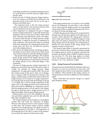
176
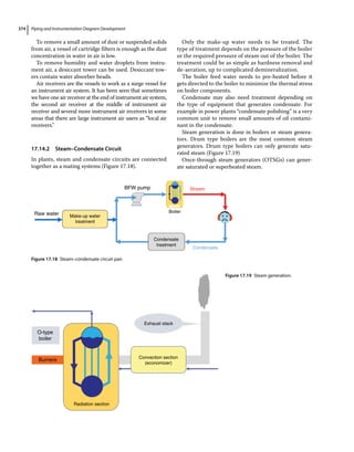
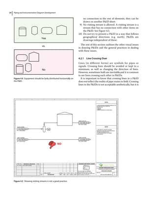
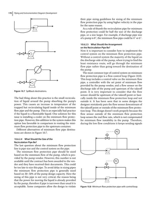
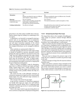
To explain the rest of the requirements for developing
a PID for centrifugal pumps, two main weaknesses
need to be discussed.
Centrifugal pumps have two main problems: cavitation
and low flow intolerance. When there is a weak point in
a piece of equipment, this should be addressed through
good process design and/or good control design.
When you are buying a centrifugal pump with a rated
capacity of 400 m3
h−1
, the seller tells you: “Thank you for
buying this and by the way, if you want to enjoy this new
pump, be careful about two things in particular (amongst
a bunch of other things!): first, this pump has a minimum
flow rate of (for example) 100 m3
h−1
, so please don’t feed
it with a lower flow rate than that.”
And second, be careful about the net positive suction
head (NPSH); this pump has a “required NPSH” of
(for example) 2 m, so please don’t feed it with a liquid
with less than 2 m of “available NPSH.”
In Section 10.6.2 these two weaknesses will be discussed
together with system process design and control design
methods to mitigate theses weaknesses.
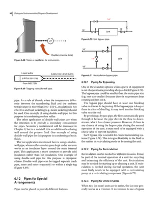
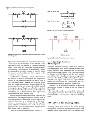
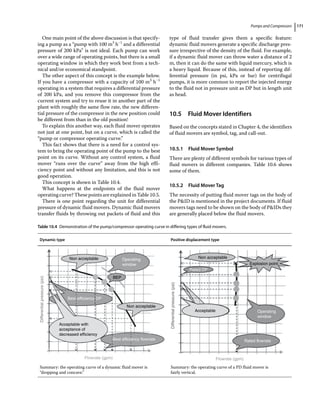
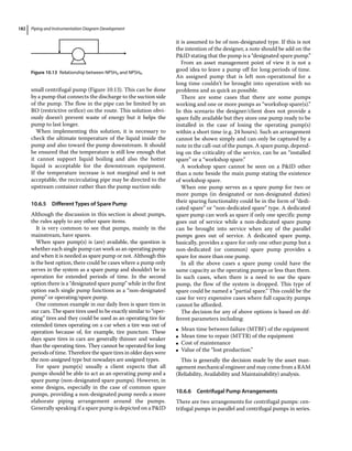
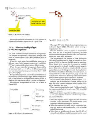
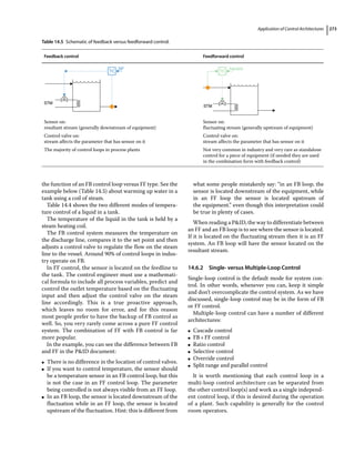
10.6.2 Low Flow Intolerance and Minimum
Flow Protection System
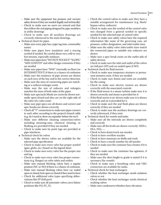
“Minimum flow rate” is a flow rate that is reported by
the pump manufacturer, and if the pump receives a flow
rate lower than that, it will start vibrating, heating up,
and in the long term the pump will experience prema-
ture failure.
A pump’s minimum flow is provided by the manufac-
turer; however, as a first, rough estimate 30–40% of the
“BEP flow rate” can be considered as the approximate
minimum flow of a centrifugal pump.
During the operation of the plant the flow rate may go
to values even lower than the minimum flow rate; how
can we protect our pump when the flow rate goes below
the minimum flow rate of our pump? To protect the
pump from flows below the minimum flow reported by
the manufacturer, a specific arrangement including a
minimum flow recirculation pipe (or “spillback”) with a
control system needs to be implemented. This system
can be called the “minimum flow protection” system.
If, for whatever reason, the flow to a pump is decreased
to a value lower than the minimum flow rate of the pump
we generally don’t have any control over increasing it if
this reduced flow rate is inevitable. What we can do is
basically a trick, and is the recirculation of a portion of
the stream around the pump to “fool” the pump into
“seeing” a flow rate higher than its minimum flow rate.
It is important to know that by recirculation of flow
around the centrifugal pump we just increase the flow
rate in one circle and include the pump but this trick
doesn’t increase the flow rate beyond the recirculation
loop, it’s upstream or it’s downstream. This technique is
named the “minimum flow protection pipe” or “minimum
flow recirculation pipe” or “minimum flow spillback.”
Now that we have learned that by recirculation we can
protect a pump against thermal and mechanical instability
during very low flow rates, a few questions should be
answered to be able to implement this trick.
The four questions that should be answered to be able
to implement a spillback system on a centrifugal pump
are:
1) In which pumps do we need to implement a recircula-
tion loop?
2) Where should we position the recirculation pipe?
3) What should be the destination point of the recircula-
tion pipe?
4) What should the size of recirculation pipe be?
5) What should the arrangement of the recirculation
pipe be?
We are going to answer all these questions one by one.
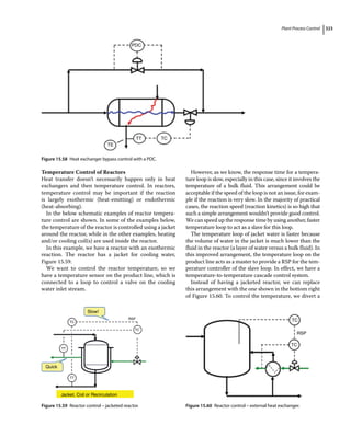
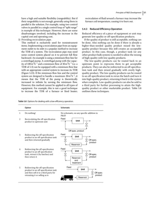
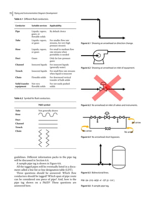
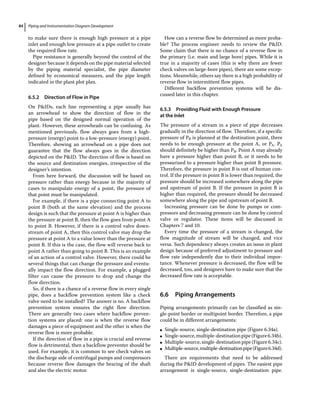
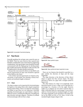
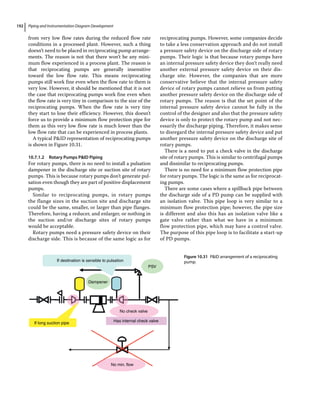
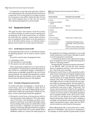
10.6.2.1 Which Pumps May Need a Minimum Flow Pipe [1]
From what it was mentioned about the requirement of a
minimum flow recirculation pipe one may believe that
this is necessary for all pumps. In practice quite a few
centrifugal pumps in a plant may have a recirculation
pipe. However, there are some cases that may not need a
minimum flow recirculation pipe. They are: pumps in
closed circulating systems, pumps in intermittent services,
small pumps, and pumps with a control valve on the flow
loop or valuable speed device (VSD).
Pumps in fully closed circulating systems may not
need a minimum flow pipe. The reason is that flow in
completely closed circulating systems doesn’t change. In
such systems there is no flow‐in or flow‐out and there-
fore flow is always constant. If flow is constant why
should we put a minimum flow pipe to protect the pump
against very low flows? Examples of such systems are hot
water systems for HVAC purposes (heating, ventilation,
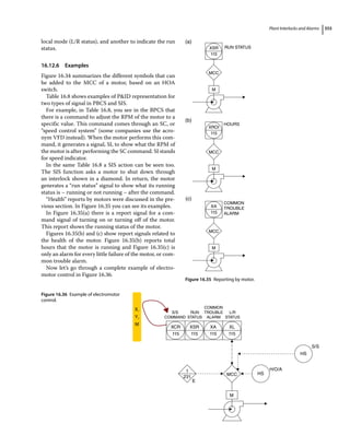
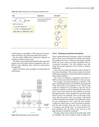
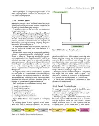
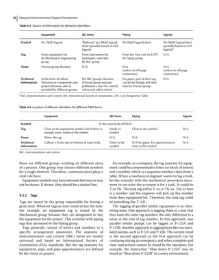
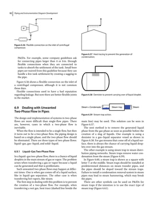
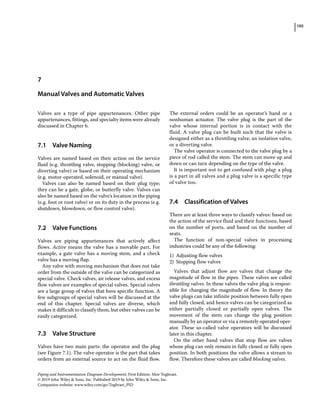
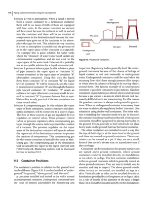
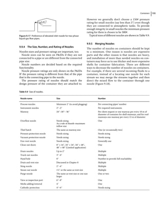
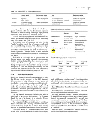
Temporary/permanent
strainer
PG for rounding
checks
To prevent
backward
rotation
As close as possible to pump
Isolation valves w/blinds
If suction flange is two
sizes smaller
PG
TSS
PG
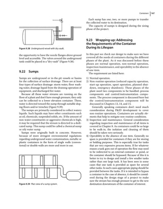
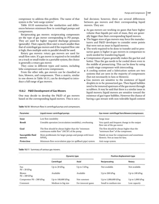
Figure 10.5 PID representation of a centrifugal pump.

195. Pumps and Compressors 177
and air conditioning). There are several other examples
of fully closed systems in the HVAC industry.
Pumps in intermittent services may not need a mini-
mum flow pipe. It is not very common to see a pump in a
plant that works in intermittent service while at a very low
flow rate. Generally speaking the problem of low flow rate
in such situations can be resolved by changing the sched-
ule of operation for the intermittent pump. There could be
a mistake in the design that an intermittent pump works at
very low flow rate, lower than the minimum flow rate. In
such cases, the design should be corrected.
We may not need to insert a minimum flow protection
pipe for very small pumps. Small centrifugal pumps, say
less than 5 hp may not need a spillback system. It is just
for the purpose of lowering the required capital cost. The
lack of implementation of a spillback protection system
for small pumps is not because they don’t see any low
flow rate. They may see low flow rates and it is detrimen-
tal for them; however, losing them and the cost of replac-
ingthemissolowthatitdoesn’tjustifytheimplementation
of a more expensive spillback protection system.
If a pump works with a flow control loop on its dis-
charge side it may not need a spillback protection sys-
tem. When a pump has a flow control loop the set point
of the loop is definitely a value higher than its minimal
flow rate. Therefore such pumps may not need a spill-
back protection system. This is the case for pumps with
a VSD on them too. If there is a VSD on a pump the rpm
of the electric model is changed based on the current
flow rate. When flow rate is low the rpm will be decreased
by the VSD system and the good news is that the required
minimum flow of the pump will be decreased accord-
ingly. Therefore, we may not need a spillback protection
systemforcentrifugalpumpswithVSDcontrol.However,
there are some companies that don’t like not implement-
ing a spillback protection system based on the idea of a
flow control loop or VSD system.
Based on the above discussion a spillback protection sys-
tem may be required for other cases. These cases are pumps
in mainstream and continuous operation, large pumps
(larger than 5 hp), and pumps with level control loops.
10.6.2.2 Where Should we Position
the Recirculation Line?
The second question that should be answered regarding
the minimum flow protection pipe is about the takeoff
point. There are primarily three points that a minimum
flow pipe can start at; upstream of the check valve,
between the check valve and the isolation valve, and
downstream of the isolation valve. The second option,
between the check valve and the isolation valve, has
no process benefit therefore we focus on upstream of
the check valve or downstream of the isolation valve
(Figure 10.6).
To satisfy the goal of a minimum flow protection pipe
the takeoff point could be either upstream of the check
valve or downstream of the isolation valve; both of
them work well. However, if the takeoff point is placed
upstream of the check valve it provides an additional
benefit. If the isolation valve mistakenly gets closed
the dead head condition (shut‐off condition) happens.
Generally speaking the dead head condition is not detri-
mental for centrifugal pumps or electric motors. It is
not even detrimental for discharge piping if the design
pressure of the piping is decided properly. However, if
one centrifugal pumping system is kept under dead head
condition for long period of time the trapped liquid will
get gradually hotter and hotter. This is because of the
addition energy of the trapped liquid through the pump’s
shaft. This increase in the temperature of trapped liquid
may not be very harmful for non‐flammable liquids;
however, if the pumping liquid is a flammable liquid
there could be the chance of fire. Because of that, a good
idea is that the minimum flow protection pipe starts
from upstream of the check valve rather than down-
stream of the isolation valve. Some companies prefer to
follow the same rule for larger pumps even when the
pumping fluid is not flammable. Their logic is that if a
pump is large the trapped liquid during the dead head
condition will quickly get hot and this is bad for the
methodology of the pump casing.
10.6.2.3 Where Should the Destination Point
of the Recirculation Pipe Be?
The next question about the minimum flow protection
pipe is the destination point. The best destination point,
which is consequently the most common one, is the
upstream container. This means that best practice is to
route the minimum flow protection pipe to the upstream
tank or vessel. However, this is not always practical and/
or economical. If the pump is very far from the upstream
container and/or the minimum flow pipe is large enough,
it is possibly not a good idea to route the minimum flow
protection pipe to the upstream container.
The other option in such situations is routing the
minimumflowpipetothesuctionsideofthepump.Insuch
situations generally the minimum flow pipe is tied in to
somewhere downstream of the suction isolation valve.
PG PG
Figure 10.6 Two potential locations of the minimum flow pipe
take‐off point.

196. Piping and Instrumentation Diagram Development
178
The bad thing about this practice is the small recircula-
tion of liquid around the pump absorbing the pump’s
power. This causes an increase in temperature of the
trapped but recirculating liquid inside of the minimum
flow pipe and the pump. This is an especially bad practice
if the liquid is a flammable liquid. One solution for this
issue is installing a cooler on the minimum flow protec-
tion pipe. However, this addition to the system makes this
option less favorable in comparison to routing the mini-
mum flow protection pipe to the upstream container.
Different alternatives of minimum flow pipe destina-
tions are shown in Figure 10.7.
10.6.2.4 What Should the Size of the
Recirculation Pipe Be?
The last question about the minimum flow protection
line is pipe size and the control system on the pipe.
The minimum flow protection pipe should be sized
based on the minimum flow of the pump, which is pro-
vided by the pump vendor. However, this number is not
available until the contract has been awarded to the ven-
dor and they have received their documents. This could
be too late to size this pipe. To avoid delay in sizing pipes
the minimum flow protection pipe is generally sized
based on 30–50% of the pump design capacity. Here the
sizing of this pipe is not very critical, the reason being
that the power for moving the liquid is already provided
by the pump, therefore if pipe is narrower than usual it is
acceptable. Some companies allow the design to violate
their pipe sizing guidelines for sizing of the minimum
flow protection pipe by using higher velocity in the pipe
for the same reason.
As a rule of thumb the recirculation pipe for minimum
flow protection could be half the size of the discharge
pipe, or a size larger. For example, if discharge pipe size
of a pump is 8″, the minimum flow pipe could be 4″ or 6″.
10.6.2.5 What Should the Arrangement
on the Recirculation Pipe Be?
Now it is important to consider how to implement the
control system on the minimum flow protection pipe.
Without a control system the majority of the liquid on
the discharge side of the pump, when trying to find the
least resistance route, will go through the minimum
flow pipe rather than going toward the destination of
the pump.
The most common type of control system on minimum
flow protection pipe is a flow control loop (Figure 10.8).
This loop includes a control valve on the minimum flow
pipe, a controller with the set point of minimum flow
provided by the pump vendor, and a flow sensor on the
discharge side of the pump and upstream of the takeoff
point. It is very important to consider that the flow
sensor should be upstream of the takeoff point or basi-
cally inside the minimum flow protection loop and not
outside it. It has been seen that in some designs the
designer mistakenly puts the flow sensor downstream of
the takeoff point or outside of the minimum flow protec-
tion loop. This design doesn’t work properly because the
flow sensor outside of the minimum flow protection
loop senses the real flow rate, which is not compensated
for minimum flow instability in the pump. Therefore,
during the low flow conditions it keeps sending signals
FC
PC
Figure 10.8 Minimum flow protection pipe with control loop.
Figure 10.7 Spillback destinations.

197. Pumps and Compressors 179
to the control valve to open and open further, and this is
why it doesn’t keep up with the low flow.
The other option is a loop similar to the flow control
loop but a pressure control loop. In this design, instead
of a flow sensor we install a pressure sensor and the loop
is a pressure loop. This control system doesn’t work for
all conditions as it only can work when the pump care is
adequately steep.
It is generally justifiable to use a control system on the
minimum flow protection pipe for larger pumps, say
larger than 35 hp.
For smaller pumps a similar system could be used, but
instead of a control system we can have an on/off system.
This means the flow sensor is still used but instead of a
control valve a searching valve can be used. Whenever
the pump flow goes below the minimum flow this valve
will be opened to recirculate some flow to increase the
pump flow rate to a value higher than the minimum flow.
As you can see this is not a very accurate way to adjust
the flow to protect the pump against the minimum flow
conditions. However, for smaller pumps, say less than 35
down to about 20 hp, it is not justifiable to use a more
expensive control loop and instead this switching loop is
used (Figure 10.9).
For smaller pumps less than 20 hp a continuous mini-
mum flow is implemented for the pump. In such cases just
a restrictive orifice (RO) could be used on the minimum
flow protection pipe (Figure 10.10).
For very small pumps, say less than 5 hp, as was men-
tioned there is no need to consider implementing a
minimum flow pipe at all.
It is important to realize that a minimum flow protec-
tion pipe is not working during the majority of pump
operation. It is because in the majority of times the con-
trol valve on the minimum flow protection pipe is closed.
This valve will be open only when the flow to the pump
goes below the minimum flow value (Figure 10.11). This
is the reason that some companies violate their pipe
sizing criteria and use higher velocity design bases for a
pipe to come up with a narrower and cheaper pipe for
this purpose.
However, the control valve on minimum flow protec-
tion pipe should be “failed‐open” (FO). This valve
should be FO because it’s function is important to keep
the pump operational. When losing the instrument air
if this valve is “failed‐closed” (FC) the pump will start
to vibrate if the flow goes below the minimum flow
value. So to keep the pump operational this valve
should be FO.
FC
Figure 10.9 Minimum flow protection pipe with switching loop.
RO
Figure 10.10 Minimum flow protection pipe with restrictive
orifice.
Senses more than 100 m3/hr
so closes the valve
Senses less than 100 m3/hr
so opens the valve
165 m3/hr
0 m3/hr FV
FV
FC
FC
FX
FX
FT
FT
FIC
FIC
165 m3/hr
Minimum flow:
100 m3/hr
20 m3/hr
80 m3/hr
80 m3/hr
Figure 10.11 Functioning of a minimum flow
protection pipe.

198. Piping and Instrumentation Diagram Development
180
All the systems on the minimum flow protection pipe
could be replaced with a device named an automatic
recirculation valve or ARC. It looks very attempting to
use a single device such as ARC instead of the more
complicated, utility dependent control system. However,
ARCs have some shortcomings. First of all they are very
prone to plugging if the service liquid is not clean. The
other limitation is that ARCs are not available in large
sizes, possibly larger than 6″. Inside ARCs are a bypass
valve and a spring‐loaded check valve. The PID symbol
for an ARC is very similar to a check valve but the differ-
ence is that the ARC symbol has two outgoing lines
(Figure 10.12).
It is important to know that not all loops around the
pumps in the PID are “minimum flow protection
pipes,” there could be similar pipes in the PID or plants
for some other reasons. A loop around the pump could
be implemented on a pump for the following reasons:
●
● As a minimum flow protection pipe.
●
● To protect the pump from gradual heating during dead
head conditions (mainly for flammable liquids).
●
● To provide fluid moving around the pump to maintain
the flow during electrical outages where the pump is
supplied by emergency electricity.
●
● To achieve an acceptable efficiency in very small cen-
trifugal pumps (less than 10 m3
h−1
).
●
● To providing a start‐up pipe for positive displacement
pumps.
If this loop around a pump is implemented for each of
above reasons, they should be sized based on different
criteria.
10.6.3 Cavitation
Cavitation is a phenomenon that is related to the genera-
tion and collapse of vapor bubbles inside of pumps.
When this happens, the pump fails prematurely
because of bubbles slamming into the impellor and the
internal side of the casing. The collective name for these
events is cavitation.
The main underlying reason for cavitation is a lack of
enough pressure on the suction side of a centrifugal
pump. When a centrifugal pump operates, it basically
“sucks” the liquid, which can generate bubbles on its
suction side, causing cavitation.
Have you tried to suck a carbonated drink out of a
tall bottle with a narrow straw? You might notice a
bunch of bubbles coming into your mouth. However,
luckily cavitation won’t happen in your mouth because
bubbles don’t have much speed!
If the liquid on the suction side of a centrifugal pump
has “enough” pressure, it won’t release gas and cavitation
won’t happen. The problem of a “lack of enough pressure
on the suction side of a centrifugal pump” can be stated
more technically as: a “lack of enough NPSH.”
NPSH or “net positive suction head” is basically the
total “effective” pressure of a liquid at the suction flange
of a centrifugal pump in “head” units (e.g. meters or feet).
Each centrifugal pump has a minimum acceptable
NPSH, which is reported by the pump manufacturer and
is termed the “required NPSH,” or net positive suction
head required (NPSHR).
A typical NPSHR for a centrifugal pump could be
a value anywhere from less than a meter, up to more
than 10 m.
After buying a centrifugal pump, the process and the
control system should be designed in order to ensure
that the liquid has enough pressure at the suction flange
to prevent cavitation. This pressure, which is provided
by the system (rather than the pump), is termed “avail-
able NPSH,” or net positive suction head available
(NPSHA), and is reported in the same units as head (e.g.
meters or feet).
This concept is shown in Table 10.7.
NPSHA should be higher than NPSHR by a pre‐selected
margin, otherwise the centrifugal pump will most likely
cavitate.
The service fluid type is part of the “system” too.
Where the pumping fluid is hotter or more volatile the
pump is more prone to cavitation.
There are, however, cases where NPSHA is lower than
“NPSHR + margin.” There different techniques available
to solve the problem. To apply some of the solutions the
designer should go back to the design stage of project but
for some others, some changes during the PID devel-
opment could solve the problem.
Each of the items in Table 10.8 need detailed evalua-
tion by process engineers and other stakeholders to
check their applicability.
A “stand pipe,” which is a solution to increase NPSHA,
is a simple vertical vessel that accumulates the liquid to a
higher level for the benefit of the downstream centrifugal
pump. The dimension of a standpipe is decided and
these rules of thumb can be used. The diameter is prefer-
able less than 24″ to be able to use a piece of pipe (seam-
less) as the body of the standpipe. The height is primarily
defined by the required level of liquid in it to provide
enough NPSHA. It is generally preferable to leave the
top of the standpipe open to atmosphere to get rid of
Figure 10.12 Minimum flow protection pipe with an automatic
recirculation valve.

199. Pumps and Compressors 181
complexities related to the need for pressure safety
valves (PSV). If this is the case, the height of the stand-
pipe should be higher to work as a “cold vent” too. If an
open top standpipe is not possible, other options should
be incorporated to make sure the design is safe.
After finishing the main topics on the development of
centrifugal pumps we deepen our understanding by
learning other concepts related to centrifugal pumps in
Sections 10.6.4–10.6.11.
10.6.4 Very Small Centrifugal Pumps
When the required capacity of centrifugal pumps is small
(say less than 10 m3
h−1
), their efficiency decreases. This
is especially true for centrifugal pumps with capacity of
less than 5 m3
h−1
. The low efficiency of such pumps is
not only bad because they are wasting energy, the pumps
also wear out more quickly. Therefore provision should
be considered to prevent that.
One solution is to buy a larger capacity pump and then
provide a continuous recirculation stream around the
Table 10.7 Relationship between NPSHA and NPSHR.
Parameter NPSHA NPSHR Comment
Provided by
Pump
N/A
Plant/System Pump manufacturer
Example 1 3 m 2 m Ok, you are good to go!
Your NPSHR is lower than your NPSHA!
You are lucky!
Example 2 1.2 m 3 m Oops!
Your NPSHA is lower than your NPSHR!
You need to do something:
1)
Ask your process engineer to somehow
increase the NPSHA
2)
Or shop around to find another less
restrictive pump with a higher NPSHR
Table 10.8 Solution for the issue of NPSHA being too close
to NPSHR.
How to increase NPSHA
Changing system features
How to decrease NPSHR
Changing pump features
●
● Raise the liquid level (e.g. using a
stand pipe)
●
● Raise the source container elevation
●
● Lower the pump and put in a pit
●
● Decrease the suction pipe length
●
● Increase the diameter of the suction
pipe
●
● Eliminate fittings in the suction
pipe as much as possible
●
● Increase the gas pressure in the
source container
●
● Use two pumps in series (booster)
●
● Decrease the liquid temperature
(e.g. by injecting cold liquid)
●
● Use a low rpm pump
●
● Use double suction
impellor
●
● Use an oversize
pump
●
● Use two smaller
pumps in parallel

200. Piping and Instrumentation Diagram Development
182
small centrifugal pump (Figure 10.13). This can be done
by a pump that connects the discharge to the suction side
of the pump. The flow in the pipe can be limited by an
RO (restrictive orifice) on the route. This solution obvi-
ously doesn’t prevent waste of energy but it helps the
pump to last longer.
When implementing this solution, it is necessary to
check the ultimate temperature of the liquid inside the
pump and also toward the pump downstream. It should
be ensured that the temperature is still low enough that
it cannot support liquid boiling and also the hotter
­
liquid is acceptable for the downstream equipment.
If the temperature increase is not marginal and is not
acceptable, the recirculating pipe may be directed to the
upstream container rather than the pump suction side.
10.6.5 Different Types of Spare Pump
Although the discussion in this section is about pumps,
the rules apply to any other spare items.
It is very common to see that pumps, mainly in the
mainstream, have spares.
When spare pump(s) is (are) available, the question is
whether each single pump can work as an operating pump
and when it is needed as spare pump or not. Although this
is the best option, there could be cases where a pump only
serves in the system as a spare pump and shouldn’t be in
operation for extended periods of time. In the second
option there is a “designated spare pump” while in the first
option each single pump functions as a “non‐designated
pump” or operating/spare pump.
One common example in our daily lives is spare tires in
our cars. The spare tires used to be exactly similar to “oper-
ating” tires and they could be used as an operating tire for
extended times operating on a car when a tire was out of
operation because of, for example, tire puncture. These
days spare tires in cars are generally thinner and weaker
than the operating tires. They cannot be operated for long
periods of time. Therefore the spare tires in older days were
the non‐assigned type but nowadays are assigned types.
For spare pump(s) usually a client expects that all
pumps should be able to act as an operating pump and a
spare pump (non‐designated spare pumps). However, in
some designs, especially in the case of common spare
pumps, providing a non‐designated pump needs a more
elaborate piping arrangement around the pumps.
Generally speaking if a spare pump is depicted on a PID
it is assumed to be of non‐designated type. If this is not
the intention of the designer, a note should be add on the
PID stating that the pump is a “designated spare pump.”
From an asset management point of view it is not a
good idea to leave a pump off for long periods of time.
An assigned pump that is left non‐operational for a
long time couldn’t be brought into operation with no
problems and as quick as possible.
There are some cases that there are some pumps
working and one or more pumps as “workshop spare(s).”
In this scenario the designer/client does not provide a
spare fully available but they store one pump ready to be
installed in the case of losing the operating pump(s)
within a short time (e.g. 24 hours). Such an arrangement
cannot be shown simply and can only be captured by a
note in the call‐out of the pumps. A spare pump, depend-
ing on the criticality of the service, can be an “installed
spare” or a “workshop spare.”
A workshop spare cannot be seen on a PID other
than a note beside the main pump stating the existence
of workshop spare.
When one pump serves as a spare pump for two or
more pumps (in designated or non‐designated duties)
their sparing functionality could be in the form of “dedi-
cated spare” or “non‐dedicated spare” type. A dedicated
spare pump can work as spare if only one specific pump
goes out of service while a non‐dedicated spare pump
can be brought into service when any of the parallel
pumps goes out of service. A dedicated spare pump,
basically, provides a spare for only one other pump but a
non‐dedicated (or common) spare pump provides a
spare for more than one pump.
In all the above cases a spare pump could have the
same capacity as the operating pumps or less than them.
In such cases, when there is a need to use the spare
pump, the flow of the system is dropped. This type of
spare could be named a “partial spare.” This could be the
case for very expensive cases where full capacity pumps
cannot be afforded.
The decision for any of above options is based on dif-
ferent parameters including:
●
● Mean time between failure (MTBF) of the equipment
●
● Mean time to repair (MTTR) of the equipment
●
● Cost of maintenance
●
● Value of the “lost production.”
This is generally the decision made by the asset man-
agement mechanical engineer and may come from a RAM
(Reliability, Availability and Maintainability) analysis.
10.6.6 Centrifugal Pump Arrangements
There are two arrangements for centrifugal pumps: cen-
trifugal pumps in parallel and centrifugal pumps in series.
Figure 10.13 Relationship between NPSHA and NPSHR.

201. Pumps and Compressors 183
10.6.6.1 Centrifugal Pumps in Parallel
For parallel arrangement of pumps there are different
arrangements including the operating‐spare arrange-
ment, the lead–lag arrangement, and simultaneously
operating pumps.
Centrifugal pumps can be arranged in parallel forms
for different reasons. They are:
●
● If the flow rate that should be handled by the pump is
huge and there is no available single pump to be used,
two or more centrifugal pump can be placed in parallel
instead of one single pump.
●
● When a higher reliability is needed: this is the case that
we need to put a spare pump in parallel with the main
pump. However, in this case there is no time that all
parallel pumps work together.
●
● When enough NPSHA is not available: sometimes the
suction side of a centrifugal pump doesn’t provide
enough NPSHA and it is close to or less than the
NPSHR one solution is using two or more smaller
centrifugal pumps. This can solve the problem
because smaller pumps have smaller NPSHR.
Figure 10.14 shows a schematic of pumps in parallel.
However, the designer should be careful about recogniz-
ing centrifugal pumps in parallel. They are not always
easy to recognize.
If there is a single pump pumping a liquid from point
A to destination B and somewhere in the middle of
discharge pipe the discharge of another centrifugal pump
is merged to the pipe, these two pipes are considered as
parallel pumps. The importance of recognizing parallel
pumps is that they usually are through one single data-
sheet. When two centrifugal pumps operating as parallel
pumps they should be completely identical. Because of
that they are usually placed in one single datasheet to
make sure they are from one single pump vendor and
they are identical.
10.6.6.1.1 Minimum Flow Pipe for Parallel Pumps
If there are parallel pumps but only one of them works at
the time and the rest are spare pumps there is no concern
about the minimum flow protection pipe. In this case,
the minimum flow protection pipe can be branched‐off
from the main discharge header of the pumps. However,
when there are operating parallel pumps the concept is a
little bit more complicated. There are at least three avail-
able options (Figure 10.15).
Option 1: one minimum flow protection pipe as a shared
minimum flow protection pipe for all the parallel
operating pumps. Although this option is acceptable
when only one parallel pump is operating at a time it
is not a good practice for simultaneously parallel
operating pumps. The reason that this is not a good
idea is that this option doesn’t necessarily compensate
the starving pump. As the parallel operating pumps
don’t have dedicated minimum flow protection pipes
if one of the pumps operating with the flow rate below
the minimum flow rate and the other pump operating
well, this system cannot work properly. This option
could be improved with a good control system. The
control system for this option will be discussed in
Chapter 14.
Option 2: Dedicated minimum flow protection pipe for
each parallel pump but with a merged pipe after the
control valve. In this option the better approach of
using a dedicated pipe and a dedicated control valve is
used; however, to save some money all the dedicated
Figure 10.14 Parallel pumps.
Figure 10.15 Minimum flow pipe for parallel operating pumps.

202. Piping and Instrumentation Diagram Development
184
minimum flow pipes will be merged together and as a
single pipe route to the destination. This option is a
technically and economically acceptable option and is
possibly the most common type of arrangement for a
minimum flow protection system of parallel operating
pumps.
Option 3: dedicated minimum flow protection system
including pipe and control system for every single
operating parallel pump. This arrangement is the
most expensive arrangement and should be used
only if the service is very critical. In this option the
system of parallel pumps are seen as their elements.
No cost saving is implemented and a minimum flow
protection pipe is implemented for each of the pumps
totally independently.
In the case that each pump has own dedicated mini-
mum flow protection pipe there could be a chance of
reverse flow. The reverse flow could be from the operat-
ing pump back to the discharge side of the idle pump
and then going to the pump in the reverse direction.
So provisions should be implemented to prevent this.
The provision is basically installing one check valve
for each minimum flow protection pipe. However, the
location of the check valve can be decided. There are
two alternative arrangements available.
Alternative A: in this alternative one more check valve
should be installed upstream of each minimum flow
branch of point. This should be done for all parallel
pumps. In this alternative there are basically two check
valves on the discharge side of each centrifugal pump;
one upstream of the minimum flow branch of point
and the other one downstream of the minimum flow
branch of point (Figure 10.16).
Alternative B: in alternative B check valves are installed
on each single minimum flow protection pipe to pre-
vent backflow. This option is a less expensive option as
the check valves should be installed on small bore
minimum flow protection pipes rather than large bore
discharge pipe in alternative 1 (Figure 10.17).
10.6.6.2 Centrifugal Pumps in Series
Sometimes centrifugal pumps should be placed in series
with each other.
It is important to recognize that centrifugal pumps in
series are not always easily noticed. One common
arrangement of two centrifugal pumps in series is the
case where a second pump takes suction from the dis-
charge of the first pump. In that case, these two pumps
also are considered as centrifugal pumps in series
(Figure 10.18).
The second reason for using centrifugal pumps in a
series arrangement is to provide a very high discharge
pressure. Generally speaking a centrifugal pump can
generate a discharge pressure of more than 3000 kPag. If
a higher pressure is needed centrifugal pumps can be
installed in a series arrangement. However, putting more
than two centrifugal pumps in a series arrangement is
Idle
isolation valves left open
Operating
Option A
Figure 10.16 Preventing reverse flow though minimum flow pipe
of parallel pumps (alternative A).
Idle
isolation valves left open
Operating
Cheaper option
Option B
Figure 10.17 Preventing reverse flow though minimum flow pipe
of parallel pumps (alternative B).
P1
P2
Figure 10.18 Pump in series.

203. Pumps and Compressors 185
not common. If there is a need to install three or more
centrifugal pumps in series to attain to a specific discharge
pressure, a better option is using a single multi‐stage
centrifugal pump. A multi‐stage centrifugal pump is
equivalent to multiple centrifugal pumps in series. In a
multi‐stage centrifugal pump each stage represents one
single centrifugal pump (Figure 10.19).
One common example of using pumps in series is when
a pump system doesn’t have enough NPSHA. One solution
for a shortage of NPSHA is to put another pump upstream
of the main pump to pressurize the ­
liquid to provide ade-
quate NPSHA for the second pump. In this arrangement
the pump with the duty of providing NPSHA is named a
booster pump and the second pump can be named things
like main pump or transfer pump. Generally speaking a
booster pump should have the same capacity (or flow rate)
of the main pipe but its discharge pressure is much lower
than that. The discharge pressure of a booster pump could
be four to seven times that of the required NPSHR or 350
kPag. One famous example is “boiler feed water system
(BFW) pumps.” BFW pumps provide high pressure water
for the boiler. As water is of generally high temperature,
the system doesn’t have enough NPSHA, therefore an
arrangement of booster pump and main pump is needed
for this purpose. From the other side, as high pressure is
needed to the boiler, two pumps could be needed.
Therefore a two pump arrangement of pumps in series
with the names of “low pressure BFW pump” and “high
pressure BFW pump” may be needed. The low pressure
BFW pump works as a booster pump and a partial pres-
surizing pump. Therefore, the discharge pressure of low
pressure BFW pump could be much higher than 350 kPag.
Here two issues regarding pumps in series are discussed:
the minimum flow protection pipe and the check valve.
From a theoretical point of view of pumps in series
only one minimum flow protection pipe is enough. The
reason is that if one pump is suffering from low flow it
will be the case for the second pump too (Figure 10.20).
Therefore there is no need for the dedicated minimum
flow protection pipe for each of the pumps in the series
configuration. However, some companies are more con-
servative and like to see dedicated minimum flow pro-
tection pipes for each single pump in series of duration.
The other point about pumps in series is if we really
need to put a check valve on the discharge side of each
of the pumps in the series configuration. Again from
­theoretical point of view one check valve is enough on the
discharge side of the downstream pump. However, if the
distance between the first pump and the second pump is
large enough, another check valve for the upstream cen-
trifugal pump may be needed. Again, some companies like
to take a conservative approach and put check valve for
each discharge site of pumps irrelevant of their distance.
10.6.7 Pump Warm‐up or Cool‐down System
For installed spares, if the ambient temperature of the space
around the pump is far from the operating ­
temperature of
the pump, the pump should be a “hot stand‐by” (or a cold
stand by in cryogenic systems) pump to make sure the
pump will not experience thermal shock during start‐up.
Suppose there are two centrifugal pumps in parallel
and one of them is an operating pump and the other one
is a spare pump. The ambient temperature is very low
and much lower than the pumping liquid temperature.
There could be a case where operating pumps work for
several days or weeks and at the same time the spare
pump stays idle without any liquid in it. In such case all
the components of the idle centrifugal pumps including
impellor, casing, etc. will stay at the ambient tempera-
ture, which is very low. Now consider the case where the
operating pump is suddenly tripped and doesn’t work
for some reason. In that case the spare pump should be
placed in operation by an operator as soon as possible.
However, by initiating the first amount of warm or hot
liquid to the cold previously idle pump the pump will
experience a very severe thermal shock. The thermal
shock is because the wide difference between ambient
temperature and the service liquid will cause cracks in
the pump casing and the other components of the pump.
Therefore, the previously idle pump could be out of work
very quickly. How can we prevent such a bad failure?
There is a practice in process plants that when the
difference between ambient temperature and the service
liquid temperature is high (say more than 100–250 °C) a
warm‐up system should be considered to prevent ther-
mal shock in the pump. This warm‐up arrangement
makes an idle pump ready for start‐up without chance of
quick failure of the pump.
M
Multistage centrifugal pump
Figure 10.19 Centrifugal pumps in series and multi‐stage
centrifugal pump symbols.
Figure 10.20 A sample PID for centrifugal pumps in series.

204. Piping and Instrumentation Diagram Development
186
There are at least two arrangements to implement the
concept of a pump system. The one which is the more
popular arrangement is shown in Figure 10.21.
In this arrangement a pipe loop bypasses the check
valve and isolation valve in the discharge site of each
pump in parallel if a spare pump is available. What this
bypass pipe can do is allow a portion of liquid from the
discharge part of the operating pump to be redirected
and go slowly to the idle spare pump from its discharge
site to its suction site. There are two important issues
regarding this arrangement: first of all the isolation valve
in the suction idle spare pump should be left open and
the second one is that the bypass pipe should be narrow
enough. The reason for installing a narrow bypass pipe is
to make sure the flow that goes in the reverse direction in
the idle spare pump is so low that it cannot back rotate
the impellor of the idle spare pump. Otherwise the pump
will be faced with some mechanical problems.
The way that we can make sure the flow to the idle
spare pump is low enough is not only installing a small
bore pipe but also putting ROs and/or a three quarter
inch needle valve to adjust the flow.
In some operating plants where a pump warm‐up
bypass line was not inserted during the design they may
solve the problem by the “duct tape” solution. This not
very ideal solution is to drill some holes in the flapper of
the check valve. The hold flapper of check valve works in
a similar way to the warm‐up bypass line. The reason
that this solution is not very good is because the drilling
generates some residual stress in the check valve flapper
that may shorten the life of the check valve.
In some designs when we deal with very high viscose
liquids an additional bypass pipe can be implemented in
addition to bypass around the isolation and check valve.
This bypass is from the discharge site of the centrifugal
pump to the suction site of the centrifugal pump with a
small needle valve on this or the RO or both of them
(Figure 10.22).
The second arrangement to provide a pump warm‐up
circuit doesn’t need anything to be implemented during
the design. Therefore, it could be a good solution if no
provisions are considered for pump warming‐up during
the design phase of the project. In this solution no addi-
tional hardware in the system is required. It only means
that the suction isolation valve of the idle spare pump is
left open together with the casing drain valve of the idle
spare pump. When an operator does that a small fraction
of flow is separated from the main flow to the operating
pump and goes through the idle spare pump and exits
from its drain valve. The bad thing about this warm‐up
arrangement is the loss of liquid from the system. In this
solution a portion of service liquid is wasted through
the drain valve of the idle spare pump. However, some
people don’t consider this as “real waste” as this wasted
liquid eventually goes to the sump system and from the
sump vessel it is returned back to the process system
(Figure 10.23).
There is the same issue when a set of operating/spare
pumps is working to pump a cryogenic liquid and the
ambient temperature is much higher than the liquid
temperature. This same arrangement should be consid-
ered to prevent the same problem of thermal chuck.
However, in this case the arrangement is named a cool‐
down pipe rather than a warm‐up pipe. Because the pur-
pose of this arrangement will be keeping the idle spare
pump at very low temperature, near the temperature of
cryogenic liquid, to make sure when it is brought into the
RO
¾”
RO
Figure 10.22 Variation of warm up arrangement 1.
Close
Open
Idle spare
Open
Open
Operating
Figure 10.21 Warm up arrangement 1.

205. Pumps and Compressors 187
operation suddenly the pump doesn’t crack because of
thermal shock.
10.6.8 Piping Spec. for Centrifugal Pumps
Depending on the generated head by the centrifugal
pump the pressure rating of the discharge flange of a
centrifugal pump could be higher than the pressure rat-
ing of the suction side and suction flange. This is not the
case for all centrifugal pumps but if the head of the cen-
trifugal pump is very high the pump manufacturer may
put a higher pressure rating for the discharge site. If this
is the case a designer may decide to choose all the ele-
ments in the discharge side of the centrifugal pump with
a pressure rating of the discharge flange. However, some
companies that have a more conservative approach pre-
fer to extend back the higher pressure rating of the dis-
charge side of the centrifugal pumps up to the suction
isolation valve of the centrifugal pump. This decision
could be an especially good decision if there are multiple
operating pumps in parallel. In that case there could be a
chance that one pump is operating and pressurizes the
suction side of the other pump (Figure 10.24).
10.6.9 Centrifugal Pump Drives
The most common type of drives for centrifugal pumps
is electric motors. However, there are some cases that
some other types of drives could be used, for example, a
diesel engine or a gas engine could be used as a drive for
a centrifugal pump. This is the case mainly for centrifu-
gal pumps in remote areas where electricity may not be
available. The other option is a steam turbine as a drive
for a centrifugal pump. It is not very common to see
steam turbines as drives for centrifugal pumps. However,
it is more attractive to use a steam turbine as a drive for a
centrifugal pump if the centrifugal pump is high power,
say more than few thousand horse power.
Companies may or may not decide to show the pump
drives. Figure 10.25 shows the PID representation of
different drives.
However any “process drives” like turbines or motors
need to be shown on the PID. It may be decided to
show a diesel motor or a gas motor in auxiliary drawings
rather than on the main process drawings.
10.6.10 (Liquid) Seal Systems in Centrifugal Pumps
Seal flush plans are supporting systems for mechanical
seals in fluid movers (pumps, compressors, blowers, and
fans). However, the question is: what is a mechanical seal?
In each centrifugal or rotary fluid mover there is a
rotating shaft that is connected to the electric motor
shaft (or the shaft of any other drive) from one side and
from the other side it is connected to the fluid mover
internals (for example the impellor). Therefore, the fluid
mover shaft penetrates through the fluid mover casing.
The penetration is done through a hole with a suitable
diameter to provide enough room for the shaft to pass
through the fluid mover casing and then to be connected
to the driver.
Now the question is how loose or how tight this
hole should be relative to the shaft diameter. If the
hole diameter is much larger than the shaft diameter
(loose system), there is always some leakage from this
gap (Figure 10.26). If the diameter of the hole almost
the same as the diameter of the shaft (tight system),
there would be no leakage because there is no gap,
but it is very difficult for the shaft to rotate in such a
tight hole.
Close
Open
Idle spare
Open
Open
Operating
Figure 10.23 Warm up arrangement 2.
Option 1: Less stringent
Option 2: More stringent
Suction pressure spec.
Discharge pressure spec.
Discharge pressure spec.
Suction pressure spec
Figure 10.24 Extension of high design pressure class to the
suction side of the centrifugal pump.
Electromotor
Steam turbine
M
D G
T
(for hp 100?)
Engine
Figure 10.25 Centrifugal pump drives.

206. Piping and Instrumentation Diagram Development
188
How can we resolve this problem?
The problem used to be resolved by application of a
stuffing box and gland. In that solution, a small space is
provided around the hole and donut shaped “packing” is
placed inside of that. The packing in the first generations
of stuffing box was a ribbon of felt. Therefore, felt from
one side prevented the leakage from the other side; it
provided enough freedom for the shaft to rotate.
The problem with a stuffing box and packing is that
there is usually some leakage from the system. The other
problem is that it needs frequent checking and inspec-
tion to make sure the packing is healthy.
This solution is still available for some pumps where
the rotation speed of the shaft is not very high or the ser-
vice is not very critical. It is interesting to know that valve
stems are still handled by stuffing box and packing.
The second solution is a “mechanical seal” which is a
more robust system. From a very simplistic viewpoint, a
mechanical seal is two blocks of graphite sliding on each
other. Both of these blocks could be in the form of
donuts. One donut is fixed in the pump casing and
around the hole and the second block of graphite is
attached to the shaft at the penetration point. During
operation of a fluid mover, these two blocks are sliding
on each other. The features of the graphite blocks are: (i)
they have very smooth surfaces and (ii) they inherently
have some lubricity features because of the nature of
graphite. Therefore, on the one hand, because of the very
low roughness of the graphite blocks surfaces, there is
almost no leakage from the system. On the other hand,
because of the oily feature of graphite blocks, the shaft
can easily rotate in the hole.
In reality, a mechanical seal is more complicated than
the above and has several other elements. The two sliding
blocks plus other mechanical parts around them is
named a mechanical seal. These days, there are more
complicated mechanical seals that are constructed of
different materials and sometimes graphite blocks are
replaced by ceramic blocks, however, the fundamental
operation remains the same.
Mechanical seals are a very critical part of every fluid
mover and need frequent inspection.
However, a mechanical seal is not something that can
be seen on a PID so why should we care about that in
PID development? Even though there is no footprint of
a mechanical seal on a PID each mechanical seal should
have a supporting system and the supporting system
should be shown on the PID. The supporting system
for a mechanical seal is a system to flush, cool down the
sliding blocks, and also lubricate those parts. Basically,
the problems associated with mechanical seals are
because there are sliding blocks, there is heat generation
in sliding block surfaces, and this generated heat should
be dissipated. By providing some sort of lubrication,
the generated heat can be decreased. The supporting
system that provides sealing, cooling, and lubrication
for a mechanical seal is named a “seal flush plan.” There
are plenty of different arrangements to provide cooling,
flushing, and lubrication for mechanical seals.
The concept of sealing systems is applicable for all
fluid movers. However, here we continue our discussion
only for pumps. More discussion on sealing systems of
gas movers is in Section 10.8.
There are different arrangements for sealing systems
of pumps, which are standardized for the sake of decreas-
ing the price and also facilitating fabrication and inspec-
tion. There is a standard generated by the American
Petroleum Institute under the name of API‐682 that
introduced more than 30 different plans as supporting
systems for mechanical seals. Usually, the mechanical
engineer in each project decides on the selected type of
seal flush plan based on standard plans stated in stand-
ards or a combination of a few of them, or even totally
non‐standard arrangements. Deciding on a specific
mechanical seal flush plan is done through the flow chart
that is provided in the standard. In standard API‐682
each seal flush plan is specified by a number. Therefore,
the seal flush plan could be introduced by seal flush plan
number 13 or seal flush plan number 15 by referring to
that specific standard.
Each seal flush plan needs a stream of fluid for the
purpose of cooling, flushing, and lubrication. This flow
stream can be provided from the process fluid, “the fluid
that is being pumped,” or from an external source. The
external source fluid can be plant water or some other type
of fluid. The final destination of each flushing/cooling/
lubricating fluid could be the process fluid or other
destinations. To make sure that we have enough flow of
Figure 10.26 Loose shaft casing touch.

207. Pumps and Compressors 189
flushing/cooling/lubricating fluid to the mechanical seal,
there is a bunch of sensors, manual valves, etc. on these
arrangements. The instruments on seal flush plan should
be tagged so that it can be captured by instrument engi-
neers. Some seal flush plans need an external utility. The
external utility could be “plant water” or other utilities.
The PID developer should make sure the required util-
ity for the seal flush plan is available. Otherwise they may
need to change the seal flush plan if possible.
Now the question is if we need to show seal flush plan
of each pump on each sheet of PIDs or not. There are
at least two ways to handle the presentation of a seal
flush plan on PIDs (Figure 10.27).
In option 1 all the arrangements related to the seal
flush plan are shown on each single pump on a PID.
In option 2, we just show a reference number beside
each pump that needs a seal flush plan and then we show
the seal flush plan arrangement in an axillary PID
drawing and tag all the instrumentation in the axillary
drawing. The second option is the better option when
the PID is crowded and showing each seal flush plan
makes it more crowded and possibly non‐usable. In the
second option, we may just show the number of the seal
flush plan number, for example the seal flush plan num-
ber 21 or 13, to refer the PID reader to the auxiliary
drawing and to the seal flush plan 21 or 13. The second
option has the advantage that all the pumps with the
same seal flush plan can be returned to one single auxil-
iary PID that shows that specific plan. In that auxiliary
PID, the arrangement can be shown and also a table
below the arrangement shows the tag number for the ele-
ment on the seal flush plan arrangement for each single
pump or compressor. This way, we can leave a bunch of
room on the PIDs.
It is important to know that not all equipment with a
rotating shaft needs mechanical seal and consequently a
seal flush plan system. In some low RPM positive dis-
placement pumps or compressors, because the speed of
shaft rotation is very low, there is no need to have a
mechanical seal, and possibly stuffing box and packing is
enough. The other example is seal‐less pumps. In seal‐
less pumps, there is no shaft that penetrates the pump
casing. The rotation of the shaft is done by magnetic
induction. Mechanical seals could also be needed for
mixers because there, there is again a shaft that’s pene-
trating an enclosed area. The mixers may need also to
have a seal flush plan, which may not necessarily be the
same seal flush plan of pumps.
The above explanation is about “liquid lubricated
mechanical seal.” There is another type of mechanical
seal named “gas lubricated mechanical seal” which will
be discussed in gas mover section.
10.6.11 Merging Pumps
Merged pumps are basically multi‐service pumps that
may have multiple destination or multiple sources. They
are attractive options from an economical viewpoint but
they are not always easy to implement.
Both multiple destination and multiple source pumps
need care in the design and PID development.
Multiple source pumps are less common than multiple
destination pumps.
When a pump gets suction from more than one source,
it is hard to predict each time which source is feeding the
pump, and this is the problem. The pressure of the source
may change during the operation and each stream from
the source to the suction of pump could be “weaker” or
“stronger” than the other stream and push the other
stream away or vice versa. One solution is to use a block
valve (manual or remotely operated) to change the source
to whatever the intention is. Otherwise, a precise design
is needed. In summary, simultaneous multiple sources
are difficult to implement while non‐simultaneous
multiple sources are easy to implement.
This again is the case for pumps with multiple desti-
nations. If streams are non‐simultaneous, they can be
easily managed by placing block valves (manual or
remotely operated) to direct the flow to whatever des-
tination. However, if the destinations need the flow
simultaneously, the design is not easy. One aspect of
the design is to make sure piping to “all” destinations
have the same design pressure equal to the dead head
pressure of the pump.
There is another non‐rare case that a centrifugal pump
is merged with a mixer! (Figure 10.28).
In this arrangement a pipe is branched off from the
discharge of the centrifugal pump and is routed back to a
container in need of mixing. Additional systems may be
needed on this pipe. For example a designer may place an
RO on this pipe to decrease the pressure.
Option 1
Option 2
Auxiliary
drawing
Process
drawing
Seal flush plan 11A
AND
Seal flush plan 11A
Seal flush plan 11A
Figure 10.27 Two ways of showing a seal flush plan on PIDs.

208. Piping and Instrumentation Diagram Development
190
However it should be realized that in this arrange-
ment, the fluctuation in the pump service impacts the
mixing and its effectiveness.
10.7 ­
Liquid Movers: PD Pumps
Positive displacement pumps are not as common as
centrifugal pumps in industry. When there is a need for
a pump in industry the first choice is a centrifugal pump
by default. PD pumps are not very user friendly and
operators generally don’t like them. In similar capacities
they are more expensive. However, they have several
advantages over centrifugal pumps. They have the least
sensitivity toward cavitation. This is the most important
advantage of PD pumps over centrifugal pumps. The
other advantage is that they are not sensitive toward a
low flow rate. They are also good if the viscosity of fluid
is high or very high and/or when a very high discharge
pressure is needed. There are two main classes of PD
pumps: reciprocating pumps and rotary pumps.
Even though PD pumps provide a lower flow rate than
centrifugal pumps in comparison with reciprocating
pumps and rotary pumps, reciprocating pumps are gen-
erally used when a higher flow rate than a rotary pump is
needed. However, the reciprocating pumps generate
lower discharge pressure than rotary pumps.
One weakness of reciprocating pumps is that they
create a pulsating flow. This pulsation is because of the
forward and backward movement of the pump’s motive
member (Figure 10.29). For example, when you are
buying a reciprocating pump whose operating pressure
is 500 psi, the pressure that is sensed by the elements
installed on the discharge side of the pump could be
between 400 and 600 psi. This is a very important
point when you decide to install sensors on the
­
discharge side of reciprocating pumps. The pulsation
can be ­
mitigated by installing a “pulsation dampener”
on the discharge side of the reciprocating pump; how-
ever, the issue still exists in the pipe upstream of the
pulsation dampener.
The issue of pulsation also exists on the suction side of
reciprocating pumps, and a pulsation dampener is some-
times needed on the suction side of them too.
Rotary pumps can work in very high viscosity services
and/or when a high discharge pressure is required.
Actually, amongst the different types of pumps, rotary
pumps can generate the highest discharge pressure but
they have the lowest capacity. One famous application
for rotary pumps is oil pumps in cars. In cars, the circu-
lation of oil is necessary for lubrication and cooling
purposes, and usually a pump is used for this. Because
the flow rate is very small and at the same time the pres-
sure needs to be high to be able to send the oil through
the capillary pipes around the cylinder blocks, the best
choice of pump here is a rotary type pump.
Rotary pumps are available in different types includ-
ing: screw pump, lobe pump, and peristaltic pump
(hose pump).
The various types of PD pumps are shown in
Figure 10.30.
However, it is important to know that not all PD pumps
can be clearly classified in one of these two classes of
reciprocating pumps or rotary pumps. One exception is
progressive cavity pumps. Progressive cavity pumps are
basically a hybrid type of PD pump. These pumps are
basically a mixture of reciprocating pumps and rotary
pumps. As these pumps were primarily invented by a
French engineer named Mono these pumps were named
by people as the Mono pump.
Inert gas
Membrane
System fluid
MT
Figure 10.29 Pulsation in reciprocating pumps.
Reciprocating pumps Rotary pumps
Piston pumps
Plunger pumps
Diaphragm pumps
Gear pump
Peristaltic pump
Progressive cavity pump
Figure 10.30 Symbols of various PD pumps.
M
Figure 10.28 Centrifugal pump also working as a mixer.

209. Pumps and Compressors 191
10.7.1 PD Pump PID Piping
As the PID arrangements for a reciprocating pump
are very different from rotary pumps the PID arrange-
ment for these two classes of PD pumps are discussed
separately.
10.7.1.1 Reciprocating Pumps PID Piping
The most important feature of reciprocating pumps is
the generation of pulsation. Reciprocating pumps gen-
erate pulsation mainly in their discharge site and also in
their suction site. If this pulsation is not desirable it
should be mitigated or dampened. Generally speaking
pulsation is more problematic in the discharge site of
reciprocating pumps. In such cases, a device named a
“pulsation dampener” should be installed in the dis-
charge site of a reciprocating pump. It is not very com-
mon to see a pulsation dampener in the suction site of a
reciprocating pump, but it has been known. We need to
put a pulsation dampener in the discharge site of a
reciprocating pump if we cannot afford pulsation. For
example, if a reciprocating pump is pumping liquid into
a huge tank, pulsation is possibly not a big deal and there
is possibly no need to install a pulsation dampener in the
discharge site of the reciprocating pump. However, it is
very important to know that without installing a pulsa-
tion dampener all the elements in the discharge site of a
reciprocating pump should be rated based on the maxi-
mum pressure that can be generated on the top of the
pressure pulse by the reciprocating pump. This means
the pressure rating of the pipe should be based on the
highest pressure generated by the reciprocating pump at
its summit of pulse. This is also the case for the other
items like pressure and temperature gauges, etc. If a PSV
needs be installed in the discharge site of a reciprocating
pump without a pulse dampener special care should be
taken to decide on the PSV set pressure otherwise the
PSV will pop up frequently.
It is important to know that the maximum discharge
pressure on the top of pulse summit is not always
reported by the pump manufacturer and sometimes this
number needs to be requested if the intention is not to
place a pulsation dampener in the discharge site of a
reciprocating pump.
A pulsation dampener is basically a small capsule that
is connected to the pipe. This small capsule is internally
split into two spaces by an elastic membrane. The top
portion of the elastic membrane is filled with an inert
pressurized gas similar to nitrogen. The bottom portion
of the capsule is filled with the discharging liquid. This
structure of a pulsation dampener helps to dampen the
pulse by pressurized gas.
There are some other items that should be considered
when developing the PID for a reciprocating pump.
A reducer or enlarger may be needed to connect
flanges of a reciprocating pump to the piping. The recip-
rocating pumps flanges could be smaller or larger than
pipe flanges in suction and discharge sites. This means
there could be a need for a reducer or enlarger or nothing
in the suction site of reciprocating pumps and it is also
the case for the discharge site. This is one important
difference between centrifugal pumps and reciprocating
pumps. If you remember, in the centrifugal pump case, in
the suction site only a reducer is acceptable and in the
discharge site only an enlarger is acceptable.
A strainer could be installed in the suction site of a recip-
rocating pump. Installing a suction strainer for a recipro-
catingpumpcouldbemoreimportantthanforacentrifugal
pump. The reason is that reciprocating pumps have more
tight clearances that can be plugged by a suspended solid
in the pumping liquid.
A pressure safety device should always be installed in
the discharge site of reciprocating pumps. This is another
important difference between centrifugal pump and
reciprocating pump PID drawing. Whether the pres-
sure safety device is a PSV or a rupture disk (RD) depends
on the situation. In Chapter 12 it will be discussed which
pressure safety device is suitable in each specific situa-
tion. The requirement of a pressure safety device is
because of the type of reciprocating pump curve. As the
reciprocating pump curve is a fairly straight and vertical
line in the case of inadvertently closing a valve in the
discharge site of a reciprocating pump (for example dis-
charge isolation valve) the pressure starts to increase and
never stops until the pump casing and/or the discharge
side piping is ruptured. The intention of installing a pres-
sure safety device not only protects the reciprocating
pump casing but also protects the piping on the dis-
charge side of the reciprocating pump. A pressure safety
device in the discharge of a reciprocating pump never
ever can be eliminated.
The lack of a discharge check valve is another differ-
ence between the reciprocating pump arrangement and
centrifugal pump arrangement in a PID context. In
centrifugal pump a check valve is always necessary to be
placed in the discharge site of the pump; however, such a
thing doesn’t need to be placed for reciprocating pumps.
The reason that reciprocating pumps don’t need a check
valve in their discharge side is because they have an
internal check valve. The internal check valve in recipro-
cating pumps prevents backflow to the reciprocating
pump in the case of sudden pump trip.
Another difference between reciprocating pumps and
centrifugal pumps is the lack of a minimum flow protec-
tion pipe in reciprocating pump arrangements. You
remember that it was mentioned in Section 10.6.1 that in
the majority of cases a minimum flow protection pipe is
needed to put around a centrifugal pump to protect it

210. Piping and Instrumentation Diagram Development
192
from very low flow rates during the reduced flow rate
conditions in a processed plant. However, such a thing
doesn’t need to be placed in reciprocating pump arrange-
ments. The reason is not that there won’t be any mini-
mum flow experienced in a process plant. The reason is
that reciprocating pumps are generally insensitive
toward the low flow rate. This means reciprocating
pumps still work fine even when the flow rate to them is
very low. However, it should be mentioned that it is not
the case that reciprocating pumps work fine even when
the flow rate is very tiny in comparison to the size of the
reciprocating pumps. When the flow rate is very tiny
they start to lose their efficiency. However, this doesn’t
force us to provide a minimum flow protection pipe for
them as this very low flow rate is much lower than the
low flow rate that can be experienced in process plants.
A typical PID representation of reciprocating pumps
is shown in Figure 10.31.
10.7.1.2 Rotary Pumps PID Piping
For rotary pumps, there is no need to install a pulsation
dampener in the discharge site or suction site of rotary
pumps. This is because rotary pumps don’t generate pul-
sation even though they are part of positive displacement
pumps.
Similar to reciprocating pumps, in rotary pumps
the flange sizes in the suction site and discharge site
could be the same, smaller, or larger than pipe flanges.
Therefore, having a reducer, and enlarger, or nothing in
the suction and/or discharge sites of rotary pumps
would be acceptable.
Rotary pumps need a pressure safety device on their
discharge side. This is because of the same logic as for
reciprocating pumps. However, some companies decide
to take a less conservation approach and do not install
a pressure safety device on the discharge side of rotary
pumps. Their logic is that because rotary pumps have
an internal pressure safety device they don’t really need
another external pressure safety device on their dis-
charge site. However, the companies that are more
conservative believe that the internal pressure safety
device of rotary pumps cannot relieve us from putting
another pressure safety device on the discharge side of
rotary pumps. The reason is that the set point of the
internal pressure safety device cannot be fully in the
control of the designer and also that the pressure safety
device is only to protect the rotary pump and not nec-
essarily the discharge piping. Therefore, it makes sense
to disregard the internal pressure safety device and put
another pressure safety device on the discharge site of
rotary pumps.
There is a need to put a check valve in the discharge
site of rotary pumps. This is similar to centrifugal pumps
and dissimilar to reciprocating pumps.
There is no need for a minimum flow protection pipe
for rotary pumps. The logic is the same as for reciprocat-
ing pumps.
There are some cases where a spillback pipe between
the discharge side of a PD pump can be supplied with
an isolation valve. This pipe loop is very similar to a
minimum flow protection pipe; however, the pipe size
is different and also this has an isolation valve like a
gate valve rather than what we have in a minimum
flow protection pipe, which may have a control valve.
The purpose of this pipe loop is to facilitate a start‐up
of PD pumps.
If destination is sensible to pulsation
No check valve
Has internal check valve
If long suction pipe
Dampener
PSV
No min. flow
Figure 10.31 PID arrangement of a reciprocating
pump.

211. Pumps and Compressors 193
A typical PID representation of rotary pumps is
shown in Figure 10.32.
10.7.2 PD Pump Arrangements
PD pumps could be placed in parallel to provide a spare
pump. However, having two (or more) PD pumps func-
tioning at the same time is not very common. Less com-
mon is using PD pumps in series.
When two (or more) PD pumps are placed in a parallel
arrangement they may need additional considerations
during PID development. Some companies put another
PSV for each PD pump in parallel to protect the suction
side of them from being over‐pressurized by the operat-
ing PD pump.
If the discharge isolation valve of the spare PD
pumps is negligently left open, the operating PD pump
pressurizes the spare pump, both on the discharge
side and suction side. Another PSV around the suction
isolation valve protects the suction side of the PD
pump (Figure 10.33).
10.7.3 Merging PD Pumps
Similar to centrifugal pumps, PD pumps may also be
used in multi‐service applications. However such appli-
cations are much less common than centrifugal pumps.
It is generally recommended to use one PD pump for
one suction source and one discharge destination.
10.7.4 Tying Together Dissimilar Pumps
Here we are talking about specific requirements when
dissimilar pumps are tied together. Such practice is not a
very good practice but sometimes can be done after con-
sidering all the requirements.
For a parallel arrangement of dissimilar pumps
(Figure 10.34) there could be different reasons for paral-
leling, similar to centrifugal pumps. However, it is not
very common to see such arrangements in process
plants. One application could be when the viscosity of
the service liquid is changing a lot and two different
pumps should be ready to be able to handle liquids with
different viscosities through two different pumps. The
other cases could be when the main pump is the centrif-
ugal pump and a small PD pump is used just to keep the
system pressurized when the centrifugal pump is off.
For a series arrangement of dissimilar pumps one rule
of thumb can be memorized: “using a PF pump as the
booster pump of another pump is not good practice.”
Different cases of this rule of thumb and its applica-
bility can be seen in Figure 10.35.
10.7.5 PD Pump Drives
The most common type of drives for PD pumps is elec-
tric motors. This is similar to centrifugal pumps.
For reciprocating type PD pumps there are, however,
some other options available.
One option is air‐operated drives. In air‐operated
drives a source of air, like plant air, is used to generate a
reciprocating movement. This reciprocating shaft is
connected to the pump shaft to operate it. Such pumps
may be named “air‐driven pumps.” This type of drive
is very common for diaphragm pumps. It should be
PSV
If you can not trust internal PSV
No dampener
Check valve
No min. flow
Figure 10.32 PID arrangement of a rotary pump.
To protect pump
Accidentally close
Operating
MT
MT
Spare
To protect low
pressure suction side Accidentally open
Figure 10.33 Additional PSVs for PD pumps in parallel. Figure 10.34 Dissimilar pumps in parallel.

212. Piping and Instrumentation Diagram Development
194
mentioned that the maximum discharge pressure of
these pumps is limited by the pressure of the air source.
The other option is used in “solenoid driven pumps.”
In “solenoid driven pumps” the drive is a stroking shaft
driven by a repeatedly magnetized solenoid.
Companies may or may not decide to show the pump
drives. Figure 10.36 shows the PID representation of
different drives.
Even if it is decided to not show pump drives, it is very
difficult to not show air‐operated drives as they are a
type of process elements.
10.7.6 Sealing Systems for PD Pumps
PD pumps similar to centrifugal pumps may need a sealing
system. However, their system is not standardized and is
designed by the vendor. If the rpm of the shaft is low
enough, the designer may decide to use packing rather
than a mechanical seal and then the need for a sealing
system is eliminated.
In a reciprocating pump the shaft is reciprocating
rather than rotating and the sealing concept could be
totally different.
10.7.7 Metering Pumps (Dosing Pumps)
Metering pumps or dosing pumps are pumps that are able
to generate flow with adequate accuracy within a reasona-
ble range of upstream and downstream pressures.
Because obviously changing upstream and downstream
pressures will change the flow rate of centrifugal pumps
they cannot be categorized as metering pumps. Metering
pumps are generally referred to as PD pumps. The majority
of metering pumps are reciprocating type PD pumps
because they have more flexibility in controlling them.
Dosing pumps may be controlled through VSD and
also change in stroke length (refer to Chapter 15).
As the amount of injected chemical is generally
important, the injecting flow rate should be checked
occasionally by operators. In the majority of cases this
is done by providing a drawdown (calibration) column
on the suction side of the pump. The rounding operator
closes the blocking valve upstream of the calibration
column and allows the pump to get suction from the
liquid inside of the column (instead of the upstream
container) and measures the time for a specific drop in
the liquid of the calibration column to calculate real
flow rate (Figure 10.37).
In some cases it is very important to install a back‐
pressure regulator. This is to mitigate one condition that
may cause uncontrolled injection of chemical to the host
stream. If the pressure of the host stream (which could
be fluctuating) goes below the suction pressure of the
Reciprocating pumps Rotary pumps
Electromotor
Solenoid
Air operated
(in diaphragm pumps)
(in diaphragm pumps)
Electromotor M
M
Figure 10.36 PD pump drives.
PG
123
Figure 10.37 PID representation of a dosing pumps.
MT MT
MT
MT
Figure 10.35 Different arrangements of dissimilar pumps in series.

213. Pumps and Compressors 195
dosing pump, the host stream “sucks” the chemical with
an unknown flow rate. To make sure that the discharge
pressure is always higher than the suction pressure, a
back‐pressure regulator needs to be installed.
10.7.8 Liquid Transfer – Summary
Where a liquid needs to be transferred and the pressure
to be compensated for (or “head” in meter units) differ-
ence is less than 50 kPag, the liquid flow is generated
only by elevating the source point (and/or lowering the
destination point) in a way to initiate a gravity flow.
Generally it doesn’t make sense to use any type of
mechanical system like a pump to transfer the liquid
where such small head is needed.
For higher required head a pump is the default choice.
In the majority of cases a pump, either centrifugal or
positive displacement, is used for liquid transfer.
The other cases are when a liquid transfer is needed
but not continuously and intermittently and very spar-
ingly. In such cases it is possible that using a pump can-
not easily be justified. In such cases liquid transfer with
the help of pressurized gas could be a good option.
One system that can work for this intention is the
“blow case” (Figure 10.38).
The main piece of equipment in a blow case system is
a container or vessel. The liquid that needs to be trans-
ferred is collected in this vessel. After a while, when
enough liquid is collected in the vessel, the liquid is
pushed out of the vessel by gas pressure. Thus, this vessel
has an inlet pipe for liquid and an outlet pipe for liquid
and each of them has a valve on it. The vessel could be
equipped with a level gauge or a level indicator.
There is another incoming stream to this vessel and it
is the motivating gas stream. This pipe also has a valve
on it.
During the collection of liquid in the vessel all valves
are closed except the valve on the incoming liquid. When
it is decided to transfer the collected liquid, the incoming
liquid valves will be closed then the incoming gas will be
opened to pressurize the system, and then the outlet
liquid gas is opened to transfer the liquid.
In some designs the operation is automated by
replacing the level indicator with a level controller and
all the manual valves with switching valves and through
a process interlock system.
If the operation is manual the operator needs to make
sure that the pressurized gas doesn’t sweep away from
the vessel and go to the liquid destination. This can be
done by closing the liquid outlet valve before completely
emptying the vessel. However, as “gas bypassing” may
happen, the pressurizing gas should be selected to
create fewer problems in the destination container. For
example if the destination container is a natural blan-
keted tank, the pressurizing gas could be natural gas,
and if it is a non‐blanketed tank, the pressurizing gas
could be plant air.
A blow case’s structure is similar to “pneumatic ejector
pumps.”
The other example of using gas to move a liquid is in
off‐loading of non‐innocent liquids from a tanker (for
example) to a tank. The transfer of hydrochloric acid
from a tanker to a tank needs an acid resistant centrifu-
gal pump, which could be expensive. A source of gas can
be used to be applied to the surface of the liquid acid in
the tanker to push it from the tanker to the storage tank.
The gas could be plant air or it could be compressed air
generated by a compressor installed on the truck.
Table 10.9 outlines some rules of thumb regarding the
selection of liquid movers.
10.7.9 Pumps: Duty Other than Pumping!
A pump can be considered as pump + valve in some
applications.
A centrifugal pump with VSD could be used as a pump
plus a control valve on a flow loop.
A PD pump with VSD could be used as pump plus a
control valve on a pressure loop with a pressure sensor
upstream of the valve (or a back‐pressure regulator).
Tank
Electricity
Pump
Blowing gas
Blow case
Tank
Figure 10.38 Transferring liquids by gas pressure through a blow case.

214. Piping and Instrumentation Diagram Development
196
It is not common to eliminate the control valve because
of the existence of the pump, but there are cases that
such thing can be done. For example when the pumping
liquid is very viscose or the pumping liquid is very
abrasive.
This concept is shown in Figure 10.39.
10.8 ­
Gas Movers: Fans, Blowers,
Compressors
For gases, there are three main types of movers: fans,
blowers, and compressors. The first two movers (fans
and blowers) are basically only for transfer or mobiliza-
tion of the gases but the third type, the compressor, is
used for mobilization and pressurization of the gas. If the
only purpose is transferring a gas from point A to point
B and there is no need to generate high pressure in the
pipe, then a fan or a blower is enough. However, if, in
addition to transferring gas from point A to point B, the
gas needs to be pressurized for the purposes of a down-
stream unit of operation or process, then a compressor
needs to be used. However it should be mentioned that
there are cases where the intention is only transferring
gas but the pressurization is also implemented to reduce
the size of the pipes.
Axial gas movers are not very popular and they have
very limited applications. Their main element is a pro-
peller, similar to a ceiling fan. One of their common
applications is in “air coolers,” to push the air across the
tube bundle to cool down the fluid flowing inside the
tubes. Axial flow gas movers are used for huge flow rates
(say more than 300 A m3
s−1
) or higher.
Centrifugal gas movers are used mainly in large
industries dealing with large flow rates of gases, up to
say 200 A m3
s−1
. The famous examples are gas process-
ing industries, including natural gas treatment and
natural gas liquids (NGL) industries.
Other than those industries, the applications for
­
centrifugal gas movers are limited. This is because
­
centrifugal fans/blowers or compressors have huge
capacities (flow rates), which are generally larger than
what is needed in most industries.
The majority of gas movers in industry are the PD type.
They are generally for capacities less than 5 A m3
s−1
.
Regarding the weaknesses of centrifugal compressors,
we may think that centrifugal compressors have the same
weaknesses as centrifugal pumps, and this assumption is
not far off. As we saw, centrifugal pumps have two big
problems: cavitation and low flow intolerance; however,
centrifugal compressors have only one problem: “low
flow intolerance.” The reason is obvious; cavitation is
only an issue when we are dealing with liquids.
10.8.1 Low Flow Intolerance and
Anti‐Surge Systems
As was mentioned, centrifugal compressors, similar to cen-
trifugal pumps, are intolerant toward low flow operations.
A system must be implemented around a centrifugal
Table 10.9 Rules of thumb for the selection of liquid movers.
Liquid mover type Driving force When?
Gravity flow Difference in elevation Where less than 50 kPag is needed to move liquid
Gas pushing transfer Gas pressure ●
● Where less frequent intermittent operation is needed
●
● Where the transferring liquid is aggressive
Dynamic pump Axial pump When flow rate is huge
Centrifugal pump Default choice
PD pump Reciprocating For low flow rates (say less than 5 m3
h−1
), and high viscosity
liquids (say more than 200 cP)
Rotary For cases more stringent than the cases for reciprocating pumps
FC
FT
FE
M
21
21
21
Figure 10.39 Pump is role of pump plus valve.

215. Pumps and Compressors 197
compressor to address this problem. The name of that
system is the “anti‐surge system.”
Table 10.10 summarizes the similarities and differ-
ences between minimum flow in centrifugal pumps and
compressors.
Reciprocating gas movers: reciprocating compressors
are the type of gas mover corresponding to PD pumps.
They are used for higher required discharge pressures
(generally). Their capacity (flow rate) is much smaller than
that of centrifugal gas movers and if the required flow rate
is high, then multiple units in parallel should be used.
Rotary gas movers: rotary gas movers are used for
small flow rates. If a gas mover is required to be installed
on a truck or small trailer in a portable system, the choice
is generally a rotary gas mover.
They come in different types and names, including
lobe compressors and screw compressors.
From the other side, gas movers can be classified as
fans, blowers, and compressors. Then a matrix, similar
to one shown in Table 10.11, can be developed to intro-
duce a full range of gas movers.
10.8.2 PID Development of Gas Movers
One may decide to develop the PID of gas movers
based on the corresponding liquid movers. This is not a
bad decision; however, there are several differences
between gas movers and their corresponding liquid
movers. They are:
●
● As gas movers are working on gases that have higher
volume than liquids per unit of mass, they are gener-
ally bigger than their corresponding liquid movers.
●
● The bigger sizes of gas movers may force the manufac-
turers and PID developer to consider some points
that were not an issue in liquid movers.
●
● The work required to be done to transfer and/or pres-
surize gases is higher in gas movers in comparison to
work needed for transferring liquid.
●
● Compression of gases generally makes the gas hot and
hotter. Thus the gas needs to be cooled down even in
the middle of pressurizing. This can be done by using
a multi‐stage compressor with intercooling.
●
● A cooling system and a lubrication system are two
systems that are seen in the majority of compressors
(but not necessarily in fans or blowers).
●
● Gas movers are sensitive to the existence of liquid
droplets in to‐be‐pressurized gas. Then liquid bubbles
need to be removed upstream of the gas mover through
scrubbers. It may be said that there is a similar issue in
liquid movers; liquid movers are sensitive toward the
existence of gas/vapor bubbles. However the chance of
having a gas stream with non‐tolerable liquid content
Table 10.10 Minimum flow in centrifugal pumps and compressors.
Parameter Liquid mover: centrifugal pumps Gas mover: centrifugal fans/blowers/compressors
Issue Low flow instability Surge issue
Result Unstable operation (recirculation instability), overheating Very quick and frequent change in the output
flow rate of the gas mover
Goal The flow should be always higher than the “minimum
continuous stable flow” (MCSF) of the pump.
The flow should be always higher than the
“minimum flow” of the compressor.
Susceptible fluid
movers
More problematic for larger pumps and pumps with lower
NPSHR
Mainly an issue for compressors and sometimes
blowers. Not an issue for fans.
Protection Minimum flow recirculation pipe (or spillback pipe) system Anti‐surge system
Table 10.11 Summary of various gas movers.
Dynamic type Positive displacement type
Centrifugal Axial Reciprocating Rotary
Fan
Pd 20 kPag
Up to 20 kPag Up to 5 kPag Not available Not available
Blower
Pd 200 kPag
Available Available Up to 200 kPag Up to 100 kPag
Compressor Pd 200 kPag Up to 100,000 kPag Not common Up to 1,000,000 kPag Up to 1,000 kPag
Comment Medium to big size For innocent gases Small to medium size Low capacity

216. Piping and Instrumentation Diagram Development
198
(wet gas) is higher than for liquids with non‐tolerable
gas content.
●
● As the gas movers are large, their moving elements
may have huge momentum and in the cases of a quick
trip in the system, they may move for a while even after
shutdown. Therefore there should be some systems to
take care of gas movers in those situations. Some of the
required actions could be implemented as part of the
interlock system. Interlock systems will be discussed in
Chapter 16.
●
● If the to‐be‐pressurized gas is flammable, more cau-
tion should be taken in design. This is mainly because
by pressurizing a gas, it will be hot.
●
● Compressors may be placed in an enclosed or
semi‐enclosed building for different reasons. One
reason could be the sound level around the com-
pressor. The other reason is to provide a dedicated
space for compressors for ease of inspection by
operators. The “compressor building” could be a
multi‐story structure for the ease of inspection and
maintenance.
10.8.3 Gas Mover Drives
The same drives of centrifugal pumps are available for
gas movers too. Electric motors, turbines (steam driven
and gas turbines), and internal combustion motors are
some of them.
10.8.4 Auxiliary Systems Around Fluid Movers
Auxiliary systems around fluid movers could be support-
ing systems for different components of the fluid mover.
A fluid mover consists of drive section and fluid mover
section. A “connection” attaches these components
together (Figure 10.40).
The “connection” could be shaft, gear box, crankshaft
or a combination.
Each of the above components may need some type of
auxiliary system. Some of these auxiliary systems are
listed in Table 10.12.
The seal type for the gas movers could be the same
type of seal types for liquid movers. The liquid mover
seal type was discussed before and is a “wet type sealing.”
For a long time it was assumed that the only type of seal
for compressors are the wet type. But later it was recog-
nized that even a gas could be used as a sealing fluid.
Then a newer type of sealing system, the dry gas seal,
came on the scene.
In a dry gas sealing system an inert gas like nitrogen
gas can be used as the sealing gas.
Drive Connection Fluid mover
Figure 10.40 Fluid mover and drive as a pair.
Table 10.12 Fluid mover auxiliary systems.
Components Type Required auxiliary system
Drive Electric motor ●
● Bearings may need cooling
●
● The majority of motor blocks are generally air cooled and no specific system is required.
However some of them need forced air cooling and air should be cooled (by air or water) and
recirculated. Some huge electric motors could be oil cooled, then a cooling system is needed
Internal combustion
engine (diesel, gas)
●
● Pistons need lubrication
●
● The motor block needs cooling
Air operated drive ●
● No specific auxiliary system is required. Only plant air should be piped
Solenoid operated
drive
●
● No specific auxiliary system is required. Only DC electricity is required
Steam turbine ●
● The block may need cooling
Gas turbine ●
● The block needs cooling
Connection Shaft ●
● The penetration point should be sealed, lubricated, cooled, and flushed
Gear ●
● Gear box may need lubrication
Crankshaft ●
● Crankshaft may need lubrication
Fluid
mover
Liquid mover ●
● Bearings may need cooling
●
● (As mentioned) penetration points should be sealed, cooled, and flushed
●
● In compressors the block should be kept cooled but this is done by the intercooler shown
on the main process PID and not the auxiliary PID
Gas mover

217. Pumps and Compressors 199
There are different types of lubrication systems
available. Their application depends of the harshness
of conditionsandalsoeconomicalconstraints.Figure 10.41
shows a few of them.
In oil bath types, there is an oil bath and the element
of interest for lubrication submerged in it or oil get
transferred to (or splashed on) it through simple parts
like “oil rings” or spoon‐type elements.
Recirculating oil type lubrication is a more compli-
cated system. A block flow diagram of a recirculating oil
system is shown in Figure 10.42.
The oil container (which may be named an oil reservoir
or oil sump) can be equipped with a heater if there is a
chance of very low ambient temperature that may “set”
the oil.
The return oil pump may not be needed in all designs.
In some designs the “return oil” can flow to the oil con-
tainer by gravity rather than through a pump. The pumps
in lubricating oils are mainly rotary pumps of types of
screw or lobe pumps.
If the heat load on lubricating is not large, the oil cooler
could be eliminated. The oil cooler could be an air cooler
or water cooler.
Where there are several to‐be‐lubricated items, the
provided oil after the cooler may go through the oil
distribution manifold and then supplied to each to‐be‐
lubricated item.
There are mainly two types of recirculating oil sys-
tem: oil sump lubrication and oil mist lubrication
systems.
In an oil sump lubricating system oil is transferred and
delivered as pure lubricant and delivered in the form of
oil droplets or jets.
In an oil mist lubricating system oil is transferred as
pure lubricant but delivered in the form of oil mist with
help and after mixing with other fluids.
There are two types of oil sump lubricating systems:
wet sump and dry sump types.
For the wet sump type an attempt is made to share
the elements of the lubrication system as much as
possible with the to‐be‐lubricated system. For exam-
ple, in all wet sump systems the oil container is not a
dedicated and external oil tank; it is rather a portion of
the to‐be‐lubricated system, which is voluminous and
has capacity to hold the lubricating oil. In some designs
the oil pump is totally independent but in others the oil
pump drives from the to‐be‐lubricated system like a
motor.
For the dry sump type the system is totally separated
and external to the to‐be‐lubricated system. An oil tank
sitting beside a to‐be‐lubricated system clearly shows the
lubrication system is dry sump type.
10.8.5 Gas Transfer – Summary
Generally speaking mechanical gas transfer is difficult
and costly. We prefer that a gas is transferred by its pres-
sure rather than using a mechanical gas mover.
The other preference is to convert the gas to liquid and
then transfer it, rather than transferring a gas!
(Figure 10.43.)
There are, however, cases where transferring gases or
vapors is inevitable. In those cases we use fans, blowers,
or compressors.
Table 10.13 outlines some rules of thumb regarding the
selection of liquid movers.
Harshness of condition
Oil lubrications
Sealed Grease lubrication Oil bath lubrication Oil circulation
Figure 10.41 Various lubrication methods depending on the harshness of conditions.
Make-up oil
Oil container Oil pump Oil filter
Oil pump
Oil cooler Lubricated
item
Figure 10.42 Block flow diagram of a recirculating oil system.

218. Piping and Instrumentation Diagram Development
200
10.9 ­Wrapping‐up: Addressing
Requirements of Fluid Movers
During the Life Span
In this section we check our design to make sure we
cover all the needs of fluid movers during each phase of
plant life. As was discussed before, these phases are
­
normal operation, non‐normal operation, inspection/
maintenance, and operability in the absence of one item.
1) Normal operation.
2) Non‐routine operation (reduced capacity operation,
start‐up operation, upset operation, planned shutdown,
emergency shut down): these phases of plant need
two components to be handled: the process compo-
nent and the control/instrumentation component.
The process component is discussed here but the
control/instrumentation component will be discussed
in Chapters 13–15.
The recirculation pipes may work as a “silver bullet”
and for such cases we have already covered them. In
other words, by recirculating fluid around a fluid
mover, we make the conditions for the fluid mover
similar to normal operation even during non‐routine
operation.
3) Inspection and maintenance: general consideration
regarding inspection and maintenance of all items is
covered in Chapter 8. Here, however, we cover the
specific requirements.
The small liquid movers may need a few items for
inspection and maintenance. However, large liquid
movers and compressors may have a bunch of points
for inspection. The minimum inspection points for
pumps could be oil level and electrical current
(amperage) reading, none of which have a footprint
on PIDs. Larger fluid movers may need temperature
sensors and vibration sensors in various locations.
4) Operability in the absence of one item: generally a
spare is provided for fluid movers. The exceptions
could be huge and expensive compressors that we
may not be able to afford to provide a spare for.­
Reference
1 Woodside O. Protect centrifugal pumps from low flow,
chemical engineering progress, June 1995, p.53.
Table 10.13 Rules of thumb for the selection of gas movers.
Gas mover type Driving force When?
Gas pressure
transfer
Gas pressure When enough pressure is
available
Dynamic gas
mover
Axial Mainly in fans
Centrifugal For huge flow rates
PD gas mover Reciprocating Default choice for
blowers and compressors
Rotary Common for blowers and
compressors
Gas or
vapor
Better
option if
doable:
Conversion
to
liquid
Pump
Point “A” Point “B”
Gas or
vapor
Conversion
to
gas/vapor
Compressor
If the first
option is
not doable,
then:
Figure 10.43 Uunfavorability of gas movers.

219. 201
Piping and Instrumentation Diagram Development, First Edition. Moe Toghraei.
© 2019 John Wiley Sons, Inc. Published 2019 by John Wiley Sons, Inc.
Companion website: www.wiley.com/go/Toghraei_PID
11.1 ­Introduction
There are mainly two types of heat transfer units: heat
exchangers and furnaces (fired heaters).
Often, stream temperatures need to be increased
or decreased in a plant in order to satisfy process
requirements.
You may say: “This is easy; I have done this a lot by
putting a kettle of water on the stove.”
You are right, but in industry there are better ways to
do this. In industry, changing the temperature of a fluid
using an external source of energy, such as fire or an
electric heater, is the most expensive method of chang-
ing the temperature, and is used as a last resort.
11.2 ­Main Types of Heat
Transfer Units
When the temperature of a stream requires increasing
or decreasing, the first choice is putting it in contact
with other higher or lower temperature streams. This
can be done in a heat exchanger.
In heat exchangers, the temperature of a stream is
changed by putting the stream in contact with other
streams to give it an opportunity for heat transfer.
When we talk about a “contacting” fluid stream, the
contacting is indirect, meaning the fluids are not mixed
together.
If the temperature of a stream needs to be increased,
then it should be sent to a heat exchanger and placed in
contact with a heating medium or a hot fluid, such as a
hot process stream, steam, or hot glycol.
If the intention is to decrease the temperature of the
target stream, it should be sent to a heat exchanger with
a cold medium, such as cold process stream, ambient air,
cooling water, or refrigearnts.
If a suitable “process stream” can be found amongst
available streams in the plant, we use it as the first choice.
Otherwise, we may have to use “heat transfer media utility
streams.”
“Utility streams” will be discussed in Chapter 17;
however, they can be briefly defined as auxiliary
streams needed by the main process in plant. A group
of utility streams are “heat transfer media utility
streams,” or the streams used to heat up or cool down
the process streams. Streams like steam, hot glycol, or
synthetic heat transfer fluids like Therminol®
are hot
utility streams that are used for heating up the process
streams. Streams like cooling water, ambient air, and
cold glycol are cold utility streams that are used for
cooling down the process streams.
If a suitable stream doesn’t exist for this purpose, or
the temperature of a stream needs to be increased exces-
sively, the other option is to use a furnace/fired heater,
which is equipment that changes the temperature of a
stream with the help of a primary source of energy, such
as fire. There are other popular names for furnaces in
industry, such as heater or boiler. If a furnace is used to
increase the temperature of water (generating vapor),
then the furnace is called a boiler.
However, increasing the temperature of a stream using
a furnace is a very expensive practice, and in industry we
try to do this temperature change using heat exchangers
as much as possible, and not furnaces. That is why in a
plant there may be many heat exchangers, but only one
or two furnaces.
This concept is shown in Figure 11.1.
When it is decided to use heat exchanger there are
questions that should be answered:
●
● Which type of heat exchanger should be used?
●
● Which heat transfer fluid should be used in the heat
exchanger?
●
● Which arrangement should be used, a single heat
exchanger, or heat exchangers in series or in parallel?
All of three above questions are generally answered in
the FEED stage of the project and there is nothing on the
shoulders of the PID development engineer. However,
here we briefly cover the topics as there have been some
cases where such decision has been delayed even to the
detail stage of project.
11
Heat Transfer Units

220. Piping and Instrumentation Diagram Development
202
11.3 ­Different Types of Heat
Exchangers and Their Selection
Different types of heat exchangers are used in the process
industry. The reason for the different available types is
the differences in indirectly contacting two fluids to
each other.
For example in shell and tube heat exchangers cold and
hot streams transfer the heat through the peripheral area
of several tubes.
The most common type of heat exchanger is the “shell
and tube” (ST HX) type. In this type of heat exchanger,
a bundle of tubes is secured on one or both sides in tube
sheets and is placed inside a cylindrical body, or shell.
A tube sheet is a perforated sheet that secures the tubes
in its holes. One fluid is flowing through the tubes
and the other fluid is flowing in the space between the
outside of the tubes and the shell.
If a tube bundle comprises only one tube, this could be
considered as a variation of a ST HX and it is named a
“double pipe heat exchanger.”
After shell and tube heat exchangers, possibly the most
common heat exchangers are “plate and frame (PF HX)
types. PF HXs provide channels for each stream.
In this type of heat exchanger, several plates are put
together in the form of a sandwich and are secured
between two “jaws.” Plates are generally in rectangular
shape. The plates are separated from each other by
peripheral gaskets, which provide a gap between every
two adjacent plates. Hot streams and cold streams flow
through these narrow gaps, or channels.
The last type of heat exchanger is the spiral type.
To visualize this type of heat exchanger, consider a PF
HX with a larger‐than‐usual plate size. If someone
rotates and wraps this “sandwich” around a core, then a
spiral heat exchanger is obtained. Spiral heat exchangers
are the least common and the most expensive type of
heat exchangers.
There are plenty of criteria that should be considered
for decision on a specific type of heat exchanger.
Table 11.1 summarizes some rules of thumb for the
selection of heat exchangers.
Another rule of thumb uses the required heat transfer
area for the selection of heat exchangers. This rule of
thumb is presented in Figure 11.2.
At the end of this section one important piece of
­
terminology needs to be discussed.
Each heat exchanger has two enclosures in contact
with each other and with a common wall.
Process heat exchanger
Utility heat exchanger
Furnace
Figure 11.1 Usage of heat transfer units in process plants.
Table 11.1 Rule of thumbs for selecting heat exchanger types.
Heat exchanger type When?
Shell and tube
(ST) heat
exchanger
Fixed
head
Default choice but applicable if
desired temperature is less than
50–60°C (or less than 80–90°C with
expansion ring)
Floating
head
Where the desired temperature is
more than 50–60°C
●
● Where the shell side fluid is
fouling
Double pipe heat
exchanger
When the decision is ST but the
required heat duty is low
Plate and frame (PF)
heat exchanger
●
● Wherever is not enough room for
an ST type but enough pressure
is available
●
● Pressure and temperature cannot
be severe otherwise the tolerance
of the gaskets of the PF HX will
be exceeded
●
● Where the required heat duty is
not certain and the modular
structure of PF helps in the
future addition of plates (and
increase in the heat transfer area)
Spiral heat exchanger For very fouling services
Aerial cooler When cooling down to
approximately 65°C is adequate
Helical coil For small heat duties, for example
sample coolers and pump seal water
heat exchangers
Helical coil Double pipe
5 m2 20 m2 1,000 m2 5,000 m2
Shell Tube-floating head
Heat transfer area
Shell Tube-fixed head
Figure 11.2 Selection of heat exchangers based on the required heat transfer area.

221. Heat Transfer Units 203
Each enclosure is for each stream, one for a cooling
stream and the other one for a heating stream.
To refer to each of these enclosures we have to use
better terminology than “closure one of the heat
exchanger” and “closure two of the heat exchanger.”
In ST HXs, a stream flows inside of tube and the
other stream flows outside of the tubes or in shell.
Therefore we can name the former enclosure the tube‐
side and the latter the shell‐side.
This applies specifically to ST HXs. The other
types of heat exchangers don’t have shells and tubes
but they still have two enclosures. Table 11.2 lists the
terminology for the two enclosures in different types of
heat exchangers.
11.4 ­Different Types of Heat
Transfer Fluids and Their Selection
As it was mentioned before we have two types of heat
exchangers of process heat exchangers and utility heat
exchangers, and process heat exchangers have higher
priority for use in plants.
We can, then, say the best heat transfer fluid is the
existing process fluid and then utility fluids.
Amongst cooling utility streams the best fluids are air
and water, which are abundant resources. Therefore they
are on the top of the list of preferred utilities. If they
cannot be used the other options can be considered.
If sea water is available it could be very attractive
choice for cooling.
A list of cooling streams is given in Table 11.3.
For heating purposes the fluids on the top of list are
hot water and steam.
A list of heating streams is given in Table 11.4.
If the temperature of the target stream needs to be
increased to more than 400°C, the only choice is probably
a fired heater.
Using steam as a source of heat in heat exchangers is
very common. However there are some points regarding
the usage of steam as a heat transfer medium.
The first point is that only saturated steam, and not
superheated steam, can work as the heat providing
fluid. If superheated steam is available, and it is
intended to be used for heating purpose in a heat
exchanger, it should be converted to saturated steam
before usage. A superheated steam is nothing except
a “gas,” but it can be converted to a heating medium
through a desuperheater.
The second point is that it should be ensured that
the steam is completely “used” in the heat exchanger
before leaving it. The complete usage of steam means
complete conversion of the steam to condensate. We
have to make sure there is no amount of steam remaining
in the stream exiting a heat exchanger. This can be done
by a placing steam trap on outlet side of the hot fluid of
the heat exchanger.
Using steam as a heat transfer medium is economically
justifiable when the required temperature of the heat
transfer medium is less than 150 °C. When the required
Table 11.2 Terminology of twin enclosures in heat exchangers.
Heat exchanger type Enclosure Name
Shell and tube (ST) heat exchanger Shell side, tube side
Double pipe heat exchanger Pipe side, annular side
Plate and frame (PF) heat exchanger Hot side, cold side
Spiral heat exchanger Hot side, cold side
Aerial cooler Tube side
Table 11.3 Utility stream choices for cooling.
Cooling streams Application
Cooling by air in
aerial cooler
When cooling down to
approximately 65°C is
adequate
Cooling by
“cooling water”
or “cold glycol”
When cooling down to 65°C
is not enough but down to
approximately 40°C is
adequate
Cooling by
“chilled water”
When cooling down to 40°C
is not enough but down to
approximately 20°C is
adequate
Cooling by
“refrigerated
water”
When cooling down to 20°C
is not enough but down to
approximately 10°C is
adequate
Table 11.4 Utility stream choices for heating.
Heating streams Application
Heating by hot
water or hot glycol
When heating up to
approximately 100°C is
adequate
Heating by steam
or “hot glycol”
When a heating up to
100°C is not enough but up
to approximately 150°C is
adequate
Heating by
non‐water based
hot liquids
When heating up to 150°C
is not enough but up to
approximately 400°C is
adequate

222. Piping and Instrumentation Diagram Development
204
temperature for the heat transfer media goes beyond this
number, using steam is not economical and possibly we
need to use another more expensive heat transfer medium,
like non‐water‐based heat transfer media. These heat
transfer media could be a synthetic heat transfer material
like Dowtherm®
.
11.5 ­Heat Exchangers:
General Naming
Heat exchangers can be named based on different
criteria.
Heat exchangers can also be named based on their
types. The most common heat exchanger types are
shell and tube heat exchangers, double pipe heat
exchangers, plate heat exchangers, and spiral heat
exchangers.
In a plant heat exchangers can be named based on
the service they are working on. A heat exchanger
could be a “gasoline heat exchanger” or a “treated water
heat exchanger,” etc. It is very common to see the
names rough heat exchanger and trim heat exchangers.
Generally speaking where there are two heat exchangers
in series and the first one is a process heat exchanger
(as will be discussed in Section 11.8.1) and the second
one is a utility heat exchanger, the upstream heat
exchanger is named a rough heat exchanger and the
downstream heat exchanger is named a trim heat
exchanger. The reason is that the first heat exchanger
brings the temperature close to the target temperature
but not very close to the acceptable temperature. The
second heat exchanger or trim heat exchanger brings
the temperature within the acceptable range.
Heat exchangers can be named based on their func-
tions. They can be named any of these four: cooler,
heater, condenser, or vaporizer.
Heat exchangers can also be named based on their
phase of the service fluids. They could be named liquid/
liquid (L/L), liquid/gas (L/G), gas/gas (G/G).
A heat exchanger can be named based on the type
of energy source or energy sink. They can be named
utility heat exchanger or process heat exchanger.
A utility heat exchanger is a heat exchanger that uses a
utility stream as a heat exchange media. The utility
stream could be steam, hot/cold, cooling water, etc.
However, in a process heat exchanger both streams are
process streams. A process stream means any stream
that is not a utility stream and is one of the streams
from the process.
For example, a heat exchanger in a plant could be a
natural gas heat exchanger, which is an ST HX, a
heater, and a gas/gas heat exchanger, and it could be
utility heat exchanger because the heating media is
utility steam.
11.6 ­
Heat Exchanger Identifiers
As it was stated in Chapter 4, the identifiers of heat
exchangers on PIDs are heat exchanger symbols, heat
exchanger tags, and heat exchanger call‐outs.
11.6.1 Heat Exchanger Symbol
It has been seen that in some companies they mistakenly
use the PFD symbol of heat exchangers instead of PID
symbols (Table 11.5).
In PFDs the symbol for heat exchangers doesn’t show
the type of the heat exchanger. This is acceptable as in
the preliminary stage of a project the type of heat
exchanger is not decided and the general symbol is used
in PDF. However at the PID stage a more specific
symbol should be used.
Table 11.6 shows symbols of different heat exchangers.
There is always confusion in recognizing and differen-
tiating between different symbols of ST HXs. That
is the reason that plenty of companies recommend
referring to the heat exchanger call‐out (rather than
the symbol) to recognize the exact type of ST HX.
11.6.2 Heat Exchanger Tag
Not all companies use heat exchanger tags. If heat
exchanger tags are needed to be shown on the body of
the PIDs, they are generally placed inside of the heat
exchanger unless there is not enough room or it causes
confusion.
Table 11.5 PFD symbols for heat exchanger types.
Heat exchanger
type
Heat exchanger
symbol
Utility heat
exchangers
Heater
Vaporizer
Cooler
Condenser
Process
heat exchanger
or

223. Heat Transfer Units 205
As it was mentioned in Chapter 4, the heat exchanger
tag could be “E‐142” or “HX‐ 430.”
11.6.3 Heat Exchanger Call‐Out
A typical call‐out for heat exchangers is seen in
Figure 11.3.
●
● The first line is the tag number of the heat exchanger.
●
● The second line is the name of the heat exchanger.
Table 11.6 PID symbols for heat exchanger types.
Heat exchanger type Heat exchanger symbol
Shell and tube (ST)
heat exchanger
Fixed head
Floating head
U‐tube
Double pipe heat exchanger
Plate and frame (PF)
heat exchanger
Spiral heat exchanger
Aerial cooler
M
Helical coil
300-E-143
Hydrocracker feed cooler
Surface area: 2,700 m2
Heat duty: 13,600 KW
Design shell: 2,800 kPag
Design tube: 2,000 kPag
MDMT shell: –45°C
MDMT tube: –45°C
Insulation: HC/64 mm
Trim shell: 3P8499-EAB
Trim tube: 3P8500-CLK
Figure 11.3 A heat exchange call‐out.

224. Piping and Instrumentation Diagram Development
206
●
● The third and fourth lines are the main characteristics of
the heat exchanger, which are the heat transferred in the
heat exchanger (heat duty) and the heat transfer area.
Heat exchangers are mainly specified by their “heat
duty,” which is the specific amount of heat transferred in
the heat exchanger. Examples of heat duties of heat
exchangers are 3.5MW (megawatts), 400kW (kilowatts),
or 100BTUh−1
.
A heat exchanger may also specified by its “heat transfer
area.” The heat transfer area of a heat exchanger is the total
area of the “metallic enclosure” inside the heat exchanger.
This area is in contact with cold fluid on one side and hot
fluid on the other side, and the heat flows through it.
A specific heat exchanger may have a heat duty of
400kW and a heat transfer area of 500m2
.
●
● Next we have design pressure and temperature,
MDMT (minimum design metal temperature), insu-
lation, and trim. However, since a heat exchanger is
basically two vessels placed inside each other (or side
by side), each of the parameters mentioned should be
listed for both of them.
In some shell and tube heat exchanger call‐outs the
TEMA (Tubular Exchanger Manufacturers Association),
type of is also mentioned. The TEMA types of heat
exchangers are a three letter acronym that specifies the
type of head, the type of body, and the type of end of the
shell and tube heat exchanger.
11.7 ­
Heat Exchanger PID
In developing a PID it is very important to draw the
PID as similar to the real plant as possible. For heat
exchangers, in the majority of cases the hot stream goes
to the heat exchanger from the top and comes out from
the bottom, and the cold stream goes to the heat
exchanger from the bottom and comes out from the top
of the heat exchanger. We have to follow this when devel-
oping and drawing the PID (Figure 11.4).
The reason for this is when a stream gets colder it
will be more dense and naturally it wants to go down,
therefore it totally makes sense to bring a hot stream to
the heat exchanger from the top and remove it from the
heat exchanger from the bottom. For the cold stream, when
it gets hot it will expand and then be lighter. Therefore to
follow the natural tendency of the flow it is better to bring
the cold stream from the bottom of heat exchanger and
remove it from the heat exchanger from the top.
This rule may have some exceptions but there are no
exceptions for condensers and evaporators.
11.7.1 Vents and Drains
Heat exchangers need vents and drains. However, as a
heat exchanger is basically two convoluted containers,
there is a need for vents and drains on each of the
enclosures. For example, in ST HXs we need vents and
drains on the shell site and vents and drains on the tube
sites. As another example we need vents and drains for
the cold side of a plate heat exchanger and also on the hot
side of the plate heat exchanger.
Vents are valves that are placed on the top of heat
exchangers and drains are valves that should be placed
on the bottom of heat exchangers. Therefore a shell
and tube heat exchanger could have one vent valve on
the top and on the shell side and the other vent valve
on the top and on the tube side and one drain valve on
the bottom on the tube side and another drain valve
on the bottom on the shell side (Figure 11.5).
Hot
Warmed cold
Cooled hot Cold
Hot
Warmed cold
Cooled hot Cold
Figure 11.4 Stream arrangements in a heat
exchanger.
Figure 11.5 Vents and drains on a shell and tube heat exchanger.

225. Heat Transfer Units 207
11.7.2 Isolation Valves
The other heat exchanger attachment could be an isola-
tion valve. Isolation valves, however, don’t exist for all
heat exchangers. The requirement for placing an isola-
tion valve for heat exchangers depends on the service of
the heat exchanger and the maintenance policy of the
plant. Some companies don’t put any isolation valves
around their heat exchangers. Their logic is that: “we
can’t afford to pull the heat exchangers out of operation
when the rest of the plant is operating thus it doesn’t
make sense for us to put isolation valves.” This logic is
not very unusual because in the majority of cases a heat
exchanger cannot be shut down and streams that used
to go inside of the heat exchanger bypass the heat
exchanger and are sent to the next equipment without
temperature change. Therefore, placing isolation valves
around heat exchangers is subjective. The other issue is
whether we really need to put bypass pipes around a
heat exchanger or not. With the same logic the majority
of companies don’t put bypass pipes around heat
exchangers because they cannot afford to send on a
stream without its temperature adjusted. One case in
which placing isolation valves and a bypass pipe around
a heat exchanger is justifiable is the case where there is
an available spare heat exchanger or the heat exchanger
is equipped with a clean‐in‐place (CIP) system or a
mechanical‐in‐place system (MIP). If a heat exchanger
is equipped with a CIP or MIP system, and the adjusted
temperature stream goes to a huge bulk of fluid down-
stream of the heat exchanger, the short period of
chemical or mechanical cleaning on the heat exchanger
can be affordable.
11.7.3 Chemical Cleaning Valves
If in‐line and in‐place cleaning is considered as part of
heat exchanger care, chemical cleaning valves should
be provided. Chemical cleaning valves are 2″ or larger
in size and can be provided as part of a heat exchanger
by the vendor, or should be provided during the PID
development stage. The chemical cleaning valves are
needed for every process fluid nozzle of the heat
exchanger (Figure 11.6).
The implementation of chemical cleaning valves may
jeopardize the concept of the isolation of heat exchang-
ers. Their installation should be taken with caution and
after getting the client’s permission.
11.7.4 PSDs
Again, as heat exchangers consist of two enclosures, both
of them should be equipped with a pressure safety device
to protect them from high pressure situations. For example,
one PSD should be placed on the ST HX and another
PSV on the tube side. The PSDs are not necessarily
installed on the shell side but rather they could be on the
connected pipe to the shell side. For tube side PSD there
is no way to install the PSD directly on the tube side
therefore the PSD is installed on the connected pipe to
the tube side of the heat exchanger.
11.8 ­
Heat Exchanger Arrangement
The arrangement of heat exchangers in a process plant
can be rigorously decided by pinch analysis. This
­
concept is beyond the scope of this book. However,
we talk about two common arrangements of heat
exchangers.
Heat exchangers can be installed in parallel or series
arrangements.
As each heat exchanger has at least two streams in it,
the concepts of series and parallel heat exchangers are a
bit complicated. When the concept of series and parallel
heat exchangers are defined, they can be regarded one
stream or two streams.
Table 11.7 shows such different arrangements. In
this figure PFD symbology is used for the sake of
simplicity.
The mixed arrangements are raised here only as a
­
deference. They are generally not used because of ineffi-
cient heat transfer in one heat exchanger.
11.8.1 Heat Exchangers in Series
Series heat exchangers could be used for different
reasons.
One reason is when the temperature needs to be
changed to a target temperature and the final temper-
ature should be precisely close to the target temperature
Figure 11.6 Chemical cleaning valves on a heat exchanger.

226. Piping and Instrumentation Diagram Development
208
selected by the designer. In such cases a “rough tem-
perature adjustment–trim temperature adjustment”
could do the job. The rough temperature adjustment is
done in a process heat exchanger and the trim temper-
ature adjustment is done by a utility heat exchanger in
series and downstream of the process heat exchanger.
The other use of series heat exchangers is when a
temperature change is needed and there are several pro-
cess streams available but none of them can solely change
the temperature to the target temperature. In such cases
several heat exchangers may be put in series so that each
of them works with one of available process streams to
finally reach the target temperature.
The third use of heat exchangers in series is to provide
a large temperature change in a heat exchanger. Generally
speaking, when a large temperature change is needed
(say more than 150°C) it cannot be handled by one heat
exchanger therefore several heat exchangers could be
placed in a series arrangement.
In the cases where several heat exchangers are placed
in series, and they are in series regarding both streams
(full series arrangement), it is very important to know
that it is always the coldest stream that is brought in
contact with the hottest stream and therefore the
arrangement of the two streams in the series heat
exchangers are against each other. This is to maximize
the heat transfer of the heat exchangers. Figure 11.7
shows this concept with PFD symbology.
In some full series arrangements the heat exchangers
are stacked up. This means that two or more heat
exchangers are placed on top of each other in a way that
a stack is created. This practice saves some of the plot
plan. This could be the case mainly where the heat
exchangers are the same size. The PID schematic of
stacked heat exchangers is shown in Figure 11.8.
In such cases there is no need to put vent and drain
valves on each single heat exchanger. We only need to
put vent valves on the top heat exchanger and drain
Table 11.7 Different arrangements of heat exchangers in series and in parallel.
Parallel Series Mixed arrangement
Regarding one
stream
Partial parallel arrangement
Partial series arrangement
Regarding
both streams
Full parallel arrangement
Full series arrangement
Figure 11.7 Arrangement of a series heat exchanger regarding
both streams.

227. Heat Transfer Units 209
valves on the bottom heat exchanger. Generally there is
not enough room to place drain or vent valves between
the stacked heat exchangers. Even chemical cleaning can
be reduced in this arrangement.
As there is generally not enough room between the
two stacked heat exchangers, the sensors can be deleted
and only the “location” for the portable sensors are left.
The concept of location for portable sensors will be cov-
ered in Chapter 13.
11.8.2 Heat Exchangers in Parallel
Heat exchangers can be placed in parallel when all of
them are operating, or in some less common cases to
provide spare capacity for the heat exchanger.
If the flow rate to a heat exchanger is huge, and/or the
required temperature change is high, a heat exchanger
with an overly high heat transfer area may be needed.
Each type of heat exchanger has a limitation on the heat
transfer area. Therefore, sometimes splitting the flow
rate and putting two or more heat exchangers in parallel
may be needed to avoid placing a heat exchanger that
needs an overly high heat transfer area. The limitation
on the heat transfer area for each heat exchanger is
­
dictated by technical and economical factors but some-
times can be deviated from. For example very large heat
exchangers with very large heat transfer areas will
require bringing a heavy duty crane to the plant when
the heat exchangers need to be sent to the workshop for
maintenance. Large cranes are not available in all plants
and usually only large plants can afford to keep them.
Therefore, we can have multiple heat exchangers in par-
allel and all of them are working, for example, 2×50%
applications.
The other case where we may have parallel heat exchang-
ers is when we need a spare heat exchanger. Generally
speaking, heat exchangers are too expensive to allow us to
keep them as a spare in plants. Therefore it is very rare to
see a parallel heat exchanger 2×100%, which means one
operatingheatexchangerandanotherspareheatexchanger.
However, in some cases, for example if the service fluid is
very fouling, we may have a spare heat exchanger.
11.9 ­Aerial Coolers
If it is decided to use ambient air as the cooling medium
on the shell side of a ST HX, the type of heat exchanger
can be used is an “aerial cooler.”
In aerial coolers, a bundle of tubes (generally finned
tubes) is secured in a frame and there is no shell at all. Air
blows through the tube bundle with the help of fan(s).
Aerial coolers have the advantage that they have no need
for a cooling medium because they use ambient air for
cooling purposes. However, they need electricity for the
operation of the motor that is connected to the fan.
Aerial coolers are generally used in multiple units in
plants.
The smallest component of an aerial cooler is the “tube
bundle.” Each tube bundle has one set of dedicated head-
ers, inlet header and outlet header. Each tube bundle
may have one or two (even up to four) inlet process flows
andthesamenumberofoutletprocessflows(Figure11.9).
A “unit” is several side‐by‐side tube bundles that work
as a single piece of equipment and carry one tag on the
PID.
Aerial coolers can be seen in process plants as “banks”,
which are large pieces of equipment. Each bank of aerial
coolers can be more than one tagged aerial cooler in a
PID. One (or more) specific area of a plant may be ded-
icated to aerial coolers and all the aerial coolers of the
plant will be located there as a “bank” (Figure 11.10).
No gauges in between
Drain
Vent
TW
PP
TW
PP
Figure 11.8 Stacked heat exchangers.
Figure 11.9 The tube bundle of an aerial cooler.
An aerial cooler bank
A unit
A unit
Figure 11.10 The unit and bank in aerial coolers.

228. Piping and Instrumentation Diagram Development
210
A plant however may have several aerial cooler farms.
A “bay” is more mechanical concept and means every
side‐by‐side set of tube bundles that have one fan in their
width
There is generally another fan on the length of each
tube bundle in the majority of cases, except in very
small aerial coolers where only one fan serves a few
tube bundles (Figure 11.11).
In the PID each single tag of an aerial cooler is a unit
and can consist of several bays and several tube bundles.
The aerial cooler banks cannot be recognized in PIDs.
A typical call‐out for heat exchangers is seen in
Figure 11.12.
●
● The first line is the tag number of the heat exchanger.
●
● The second line is the name of heat exchanger.
●
● The third and fourth lines are the main characteristics
of the heat exchanger, which are the heat transfer
area and the heat transferred in the heat exchanger
(heat duty).
●
● Next there is design pressure and temperature, MDMT
(minimum metal design temperature), and trim.
●
● The last item is the driver power. The driver is generally
an electric motor.
The number of bays may also be mentioned in the
aerial cooler call‐out.
11.9.1 Aerial Cooler PID
As each aerial cooler may have several tube bundles
thus the process flow should be evenly distributed
amongst them. Therefore flow distribution is a critical
issue. To provide a good distribution – and collection –
the distribution headers are placed above the bank of
aerial coolers and the collection headers below the cool-
ers are placed (Figure 11.13).
As the PID is a 2D diagram and is generally a plan
view, it is not always easy to show the headers. In some
PIDs the distribution header and collection header are
completely ignored and left on the shoulders of pipe
modelers to “recognize” the existence of them. In some
other PIDs the cross section of the header is shown
(Figure 11.14).
The other details of aerial coolers are drains and vents,
isolation valves, and pressure safety devices (Figure 11.14).
Each tube bundle of an aerial cooler needs drain and
vent capability. Sometime the aerial cooler by itself has
drain and vent valves on its headers. However this is not
the case for all aerial coolers. Then, the designer may
A small bay with one tube
bundle and one fan in width
A bay with three tube bundles
A bay with two tube bundles
Figure 11.11 Definition of bay.
DRIVER: KW
DP/DT: 1300 KPag/FV @ 180°C/–29°C
HEAT DUTY: 7,100 kW
BARE SURFACE AREA: m2
22-AE-0013
SPILLBACK COOLER
Figure 11.12 An aerial cooler call‐out. Figure 11.13 Flow distribution in aerial coolers.

229. Heat Transfer Units 211
need to provide air and drain valves on the connecting
pipes of an aerial cooler. If this is the decision it is appro-
priate to provide one set of vent and drain valves on
each header of a tube bundle. This means that each
tube bundle has two vent valves on the top of each header
and two drain valves on the bottom of each header.
An aerial cooler can also be equipped with isolation
valves.
As the tube bundle of aerial coolers is considered as an
enclosure, it should be protected from over‐pressuriza-
tion by installing PSDs.
11.9.2 Dealing with Extreme Temperatures
As aerial coolers use ambient air generally without any
pre‐treatment, they thus should be robust. There are,
however, some extreme cases that should be considered
in the design of aerial coolers and/or in the PID devel-
opment of them. The main important issue is extreme
ambient air temperatures.
The ambient temperature change depends on seasons
and going from night to day or vice versa. The control
system around an aerial cooler tries to compensate the
ambient air temperature so that there is a fairly fixed
temperature of process fluid exiting the aerial cooler.
Such a control system will be discussed in Chapter 13.
Here, however, we talk about methods to deal with
“extreme” ambient temperatures; how handle the cases
where the ambient air is extremely high or extremely low,
which may causes frosting if there is enough vapor in the
air. If such conditions are forecastable in the area, it
should be considered in the design.
●
● Dealing with extremely low temperatures: extremely
low temperatures (say less than 15–20°C) could be
problematic, mainly where there is a chance of frosting
on the aerial cooler tubes. There are mainly two ways
to handle such conditions: using a steam coil and warm
air recirculation.
In the steam coil solution, a bundle of steam coils is
superimposed on the aerial cooler bundles. By doing
this, the air moving through the aerial cooler bundle
has to go through the steam coils at the beginning.
This warms up the cooling air and prevents frosting.
In the warm air recirculation solution, instead of
“virgin” ambient air, the warmed ambient air is used
for cooling purposes in the aerial cooler.
There could be two sources of warmed up air.
In “internal air recirculation” the source of warmed up
air is the already used ambient air after some cooling
effect on the aerial cooler. In “external air recircula-
tion” the source of warmed up air is partially from the
“airconditionedair”oftheadjacentbuilding.Obviously
the external air recirculation is available only for aerial
coolers in the vicinity of air‐conditioned buildings.
Implementing the concept of air recirculation needs
putting several louvered walls around the aerial cooler
in a way that it looks like the aerial collar is placed
inside of a “box” with perforated walls.
One example of a boxed aerial cooler is shown in
Figure 11.15.
A combination of steam coil and recirculation air
can also be used.
In the PID, the louvers should be shown and
tagged in a similar way to control valves.
●
● Dealing with extremely high temperatures: I have seen
in extremely hot days of summer that water hoses have
been placed on the aerial cooler bundles! However a
factory‐built system to deal with extremely high
temperature is a “humidifier aerial cooler.”
11.9.3 Aerial Cooler Arrangement
Aerial coolers in series are generally avoided. This is
because of difficulties in the symmetrical distribution
and collection network between two aerial coolers in
series considering the limited available space. However it
is not difficult to avoid aerial coolers in series. By using
several aerial coolers in parallel (which is very easy) and
also using a multiple pass configuration, series aerial
coolers can easily be avoided.
As aerial coolers have a modular structure, in the major-
ity of cases they are installed in a parallel arrangement.
Represent distribution header
Represent Collection header
Figure 11.14 PID detail of an aerial cooler.

230. Piping and Instrumentation Diagram Development
212
There are, however, applications where an aerial cooler is
used for very small heat duties, which need only a single
bay aerial cooler.
11.10 ­
Merging Heat Exchangers
Even though heat exchangers are expensive pieces of
equipment they are not generally merged. The reason is
that the design of heat exchangers is so specific that it is
not easy to find one heat exchanger that matches two
different services.
11.11 ­Wrapping‐up: Addressing
the Requirements of a Heat
Exchanger During its Life Span
In in this section we check our design to make sure we
have covered all the needs of heat exchangers during
each phase of plant life. As was discussed before, these
phases are normal operation, non‐normal operation,
inspection/maintenance, and operability in the absence
of one item.
1) Normal operation of heat exchangers: the required
considerations are already covered.
2) Non‐routine operation (reduced capacity operation,
start‐up operation, upset operation, planned shut-
down, emergency shut down): these phases of plant
needs two components to be handled: the process
component and the control/instrumentation compo-
nent. The process component is discussed here but
the control/instrumentation component will be
discussed in Chapters 13–15.
One main issue regarding heat exchangers is that
when flow goes below a specific value, the heat
transfer is decreased. If there are heat exchangers in
parallel it may be decided to pull one unit out of
operation to keep the adequate flow rate in the
­
second parallel heat exchanger. However, if there is
no parallel unit, it is not easy to mitigate the problem
of a very low flow rate.
3) Inspection and maintenance: general consideration
regarding inspection and maintenance of all items
will be covered in Chapter 8. Here, however, we cover
the specific requirements.
There could be a piping arrangement to allow
“back‐flush” of a heat exchanger during normal oper-
ation. This back‐flush arrangement can be placed on
cooling water to remove fouling from the water side
of the cooler (Figures 11.16).
4) Running the plant in the absence of pipe: There is
generally no consideration for the times that a heat
exchanger is out of operation. The reason is that heat
CWR
CWS
CWR
CWS
Figure 11.16 Back‐flushing in heat exchangers.
VIEW VIEW VIEW
PLAN
Winter Operation
PLAN
Summer Operation
PLAN
Schematic of system
Figure 11.15 Aerial cooler with the air recirculation concept implemented.

231. Heat Transfer Units 213
exchangers are expensive pieces of equipment. When
a heat exchanger is out of operation, it generally
impacts the operation.
11.12 ­
Fired Heaters and Furnaces
Furnaces are the least favorite heat transfer units for dif-
ferent reasons; they are expensive and they have a bunch
of safety issues to be addressed. They may have names
other than furnace; when the process fluid is water, they
are named boilers or steam generators.
The main component of every furnace is the heating
system. There are mainly two types of furnaces: fired
heaters where the heating system is fire, and electric
heaters where the heating system is an electrical element.
Electrical furnaces are expensive from a capital cost and
operating cost viewpoint and are not used unless a very
high temperature is needed. Therefore our discussion is
limited to fire heaters.
Fire heaters use fire to increase the temperature of pro-
cess fluids. Fire is generated in burners where fuels and
oxidant are brought together. The fuel could be anything
from oil, gas, or coal to some specific sludge. The oxidant
is mainly air and sometimes other oxidants like oxygen.
The result of burning fuel is flue gas. There are some
furnaces where their source of energy is not burning fuel
but electrical energy.
Therefore, a furnace has at least three systems that
should be taken care of during the PID development:
the process fluid side, the firing side, and the flue gas side
(Figure 11.17).
11.12.1 Process Fluid Side
As it was mentioned, for efficient heating, the fluid
should be exposed to heat with narrow thickness.
However, there are some cases where a huge stream
needs to be heated in a furnace. In such cases the stream
is split into several narrow bore pipes before entering the
furnace. This multi‐pass arrangement is needed to make
sure the coils inside the fired heater have a small enough
diameter (generally less than 4–6in.) to make sure heat is
absorbed effectively by the process fluid. Therefore each
fired heater may warm up a stream, not through a single
coil, but rather through several narrow bore coils of gen-
erally less than 4–6in. Each coil circuit in a furnace is
named one “pass.” We may have a furnace with 2, 4, 6,
etc. passes. Therefore, a large‐bore pipe for a process
fluid is split into 2–6 (or more) small‐bore pipes outside
the fired heater, and then all of them enter the fired
heater chamber. These multiple passes will merge
together again on the other side of the fired heater after
heating the process fluid.
One responsibility of the PID developer is to distrib-
ute the stream of interest for heating amongst several
coils evenly. This can be done by a control system or by
symmetrical piping. These solutions are briefly discussed
in Chapter 6 and the control system is discussed in more
depth in Chapter 15.
Furnaces are designed and built to handle large
thermal expansion of its elements because of large
temperature changes. However furnaces cannot handle
the thermal shock. Introducing cold process fluid into
the furnace coils may cause thermal shock and initia-
tion of cracks and rupture in the furnace coils. Because
of that when the temperature difference between the
cold process fluid and the furnace target temperature is
more than 100°–150°C, preheating may be needed.
This preheating could be necessary to bring the cold
process fluid to a temperature closer to the furnace
temperature. The preheating is generally done by a heat
exchanger and more commonly this heat exchanger
uses the hot process fluid exiting the furnace to heat up
the cold process fluid entering the furnace. Sometimes
preheating is done through heat exchange from the hot
flue gas of the furnace.
11.12.2 Flue Gas Side
Flue gas is generated inside the furnace and directed to
the atmosphere through the stack.
A fired heater is a heat transfer unit that uses fire to heat
up the temperature of a process fluid.
If a fired heater is intended to be used to change the
process fluid physically or chemically to other fluids by
heating up, it can be named a furnace.
Air
Fuel
Firing System
Process fluid
Flue Gas
Figure 11.17 Three fluid streams within a fired heater.

232. Piping and Instrumentation Diagram Development
214
Flue gas generally finds it way out of the furnace box by
going up. Flue gas is hot and an adequately long stack
provides enough draft (natural draft) to suck the flue gas
out of the furnace box. The other option of removing
flue gas from the fired heater box is placing a fan to suck
the flue gas to the outside or an “induced draft” system.
As the flue gas is hot, releasing it to the atmosphere
means losing energy. Thus, it is not rare to see another
set of coils in the flue gas route toward the stack to
use – at least a portion of – the flue gas energy.
One common problem of coils in the flue gas route is
soot accumulation. Accumulation of soot around the
external wall of the flue gas coils decreases the heat trans-
fer and also may cause overheating in some spots of the
coils. Soot blowers are briefly discussed in Chapter 8.
A soot blowing system is placed to remove the accumu-
lated soot at specific intervals. Soot blowers work intermit-
tently based on a pre‐determined schedule. Their operation
happens during the normal operation of a furnace and with-
out major interfere. Soot blowers generally spray steam
toward the coked coils to remove the soot.
Generally things in the route of the flue gas are installed
on furnaces and we don’t need to add anything on the
PID.
11.12.3 Firing Side
Having fire in the process element looks a very scary
thing. That is the reason why there are bunch of provi-
sions to make sure the fire is under control at all times.
Some of these provisions are provided by a safety instru-
mented system (SIS) and some others are provided by
good design. The SIS is discussed in Chapter 15.
The firing side comprises at least two separate systems:
the fuel side and oxidant side.
Fuel is brought to the burners through a fuel distribu-
tion system. Two very common fuels for furnaces are fuel
oil and fuel gas. If the fuel is coal, it should be brought near
the furnace, not through the utility network, but through
other methods, which are beyond the scope of this book.
If the oxidant is air, it could be brought to the burner by
natural draft, forced draft, or only relying on the induced
drafting system of the flue gas.
The air could be pre‐heated through coils in the convec-
tion section of the fired heater for more efficient burning.
The firing happens in burners. As fuels are commonly
fuel gas or fuel oil there are fuel oil burners and fuel gas
burners. There are also burners that are designed to use
either of those fuels and thus are “dual fuel burners.”
Because in microscopic scale fire happens in the vapor
phase (rather than the liquid phase), the fuel oil – and not
the fuel gas – should be converted to vapor or something
else easily convertible to vapor. As converting fuel oil to
vapor is a very energy intensive operation we prefer to
convert them to small droplets, which can then be easily
evaporated in the temperature provided by firing.
Therefore, all fuel oil burners need a type of “atomization.”
From a theoretical viewpoint, to convert a continuous
fluid to discrete droplets you need to exert energy in it.
The energy for atomization can come from a high pres-
sure stream or by a mechanical device. Amongst high
pressure fluid atomization systems we have pressure jet
atomization (with pumped fuel oil), stream atomization,
and air atomization. The whole purpose of a discussion on
atomization here is to point out that sometimes the PID
developer needs to bring another stream (other than fuel)
to the burner for the purpose of atomization.
Burners need a “pilot flame” to help the firing as soon
as it is ordered to do so. If you go down deep to the the-
ory of fire you will see that starting a fire depends heavily
on probabilistic phenomena. This means when every-
thing is ready to start a fire (which means the fire triangle
is available), it may take a “short time” to start firing. This
short time could be acceptable when you try to fire your
barbeque but in large furnaces, releasing a fuel and air
mixture without fire is dangerous. Therefor each burner
is equipped with a small flame near the main burner tip,
which is fueled by an easy‐to‐get‐fire fuel (generally fuel
gas) separate from the main fuel pipe. This small built‐in
burner is named a “pilot.” Therefore during PID devel-
opment fuel gas is also needed for the pilots from a
separate network.
As mentioned before the fuel to burners are provided
by fuel gas or fuel oil utility distribution networks.
Figure 11.18 shows a typical summarized PID of the
fuel route to a burner.
Isolation valves should be provided right after the fuel
header, before the burner header and upstream of each
burner.
Small valves should be provided (at least two) for
draining, venting, and or purging the pipe.
The fuel preparedness block could be different things
depending on the type and condition of the fuel. It could
consist of a pressure regulator to drop the pressure to
a fairly constant pressure. A fuel filter could also be
here if the fuel could have particles that could plug the
burner tips.
Blocks of switching valves are provided on the fuel
sub‐header and on each burner branch. In some designs
two switching valves are used in series to satisfy the
required safety level. In some older designs there was
no additional set of switching valves on each burner
branch.
A block consisting of a control valve station, is pro-
vided on the pipe in series with the switching valve block.
The pilot gas route doesn’t need a control valve station
but it still needs a switching valve.
It is very important to mention that in plenty of juris-
dictions BMS (burner management system) is a code and
therefore firing systems are highly regulated.

233. Heat Transfer Units 215
Generally speaking there is more than one burner in
each fired heater, therefore a burner header may be
needed. It is very important to provide the fuel to several
burners of a fired heater with the same flow and pres-
sure. This required distribution is specific to the fuel
pipe of burners.
It discussed in Chapter 17, there are two main types of
flow distribution, tree type and loop type. As there is
more chance of pressure and flow swinging in fuel
oil – rather than fuel gas – the fuel oil is distributed
amongst the several burners of a fired heater through a
loop distribution. A ring header around the furnace pro-
vides a fairly even fuel oil for the burners.
Figure 11.19 shows the PID of a fuel gas burner with
pilot gas.
As part of SIS, if for whatever reason the flame put off,
the unburnt fuel‐air mixture inside of furnace should be
displaced as soon as possible. The steam can be used for
this purpose. This steam is known as “snuffing steam.”
11.13 ­
Fire Heater Arrangement
Fired heaters are rarely placed in series or parallel. Fired
heaters are such expensive pieces of equipment that it is
preferred to only have one of them in service.
Burner
To BurnerTo Burner To Burner
To Burner To Burner
To Burner
To Burner
To Burner
Duplex Filters
Duplex Filters
Natural Gas header
ANOTHER Natural Gas header
To Burner
PT
123
PC
123
SD
SD
SD
SD
Majn gas ring Pilot gas ring
Fuel Gas
Fuel gas ring for one fired heater
Fuel gas ring for one fired heater
Pilot Gas
Figure 11.18 PID of a fuel gas burner with pilot gas.
Control Valve Station
Fuel Peparedness
Burner
Burner
Burner Header
(for each heater)
Safety Shutdown
Valving System
Safety Shutdown
Valving System
Safety Shutdown
Valving System
Figure 11.19 Fundamentals of the fuel route to burner.

234. Piping and Instrumentation Diagram Development
216
However there is a very common case in which a heat
exchanger and a fired heater are in series.
The logic for heat exchangers–fired heaters in series is
the same as for heat exchangers– heat exchangers in
series mentioned before; if a large temperature jump is
needed (say more than 150°C), heat exchangers–fired
heaters in series may be needed to prevent any thermal
shock in the fired heater.
11.14 ­
Merging Fired Heaters
Furnaces are generally not merged together because
each of them is tailor‐made for the requirements of each
stream.
11.15 ­Wrapping‐up: Addressing
the Requirements of Fired Heaters
During their Lifespan
In in this section we check our design to make sure we
cover all the needs of containers during the defend phases
of the plant. As was discussed before, these phases are
normal operation, non‐normal operation, inspection/
maintenance, and operability in the absence of one item.
The requirements are checked here:
1) Normal operation: the required considerations are
already covered. One important item for fired heaters
is “peep holes”, which provide a means for the field
operator to check the flame.
2) Non‐routine operation (reduced capacity operation,
start‐up operation, upset operation, planned shut-
down, emergency shut down): these phases of the
plant need two components to be handled: the process
component and the control/instrumentation compo-
nent. The process component is discussed here but
the control/instrumentation component is discussed
in Chapters 13–15.
Because there is fire inside of fired heaters there
are plenty of safety measures around them.
Although the majority of them are already imple-
mented by the vendor, it is important to study each
of them before implementing them in the PID to
make sure they follow the codes and/or client safety
rules.
3) Inspection and maintenance: general consideration
regarding inspection and maintenance of all items is
covered in Chapter 8.
There are plenty of activities regarding fired heater
and boiler inspection and maintenance. One main
activity is regarding the integrity of the refractory
layer inside of the firing box.
4) Operability in the absence of one item: there is gener-
ally no spare provided for fire heaters as they are very
expensive process items. If for whatever reason a tank
goes out of operation the unit may need to be shut
down.

235. 217
Piping and Instrumentation Diagram Development, First Edition. Moe Toghraei.
© 2019 John Wiley Sons, Inc. Published 2019 by John Wiley Sons, Inc.
Companion website: www.wiley.com/go/Toghraei_PID
12.1 ­Introduction
In Chapter 7, different safety related valves were discussed.
Here we talk about the detail of pressure safety valves.
12.2 ­
Why Pressure Is So Important?
As mentioned in Chapter 5, in each plant for each single
piece of equipment there could be five process parame-
ters that are swinging. For each parameter there are
guards to limit the extent of swing and to push back the
parameter to its normal level. Placing mechanical relief is
the last guard before the occurrence of a disaster
(Figure 12.1).
The process parameters are flow, level, pressure, tem-
perature, and composition. As the most common
mechanical relief is the “pressure safety valve” you may
ask what is more important about pressure than the
other process parameters (Figure 12.2).
The point is that changing every single process param-
eter will change the pressure.
Increasing the flow in a pipe will increase the pipe
pressure.
Increasing the liquid level in a container will fill the
container and eventually increase the pressure of the
container.
The increasing temperature may be twofold. On the
one hand, by increasing the temperature generally
the ­
fluids expand and they will increase the pressure.
On the other hand, the higher temperature generally
­
weakens the body wall of the process element enclosing
the fluid and makes the enclosure easier to burst.
Changing the composition not always, not quickly, and
not directly affects the occurrence of a high pressure
­
disaster. One example of the effect of composition
change on high pressure disaster is when the composi-
tion of a non‐acid resistant vessel suddenly turns into an
acid. In this case the vessel wall becomes corroded and
gets thinner and ready to burst.
12.3 ­Dealing with Abnormal
Pressures
Abnormal pressure here means any over‐pressure or
under‐pressure conditions happening for enclosures.
Generally speaking, to deal with any issue there are
four different solutions available: (i) inherent solution,
(ii) passive solution, (iii) active solution, and (iv) proce-
dural solution.
For example, if the problem is “infectious diseases,”
there are a few solutions available:
●
● Inherent solution: relocating to another planet with no
such diseases
●
● Passive solution: increasing the strength of your body’s
immune system
●
● Active solution: taking medicine when you get sick
●
● Procedural solution: follow this procedure: “don’t go to
tropical areas”.
Similarly, there are four different groups of solutions
available when dealing with over‐ or under‐pressure
­
situations. Each of them have their own set of costs and
benefits, and some are more suitable than others for
­various situations.
●
● Inherent solutions: An inherent solution is simply the
elimination of the problem, or the conditions that
cause the problem. In the case of removing overpres-
sure, an inherent solution is “either not working at
high pressure at all, or not using any enclosed system.”
The inherent solution is often not generally within
the realms of possibility. However, this solution can be
used to decrease the extent of the issue, by using a
low‐pressure process rather than a high‐pressure one.
Such a change could be costly and may only be imple-
mentable in the very early stages of a project.
●
● Passive solutions: passive solutions typically take the
form of fortifying the affected elements before they are
exposed to the problem. In a plant, a passive solution
for high pressure is to design all the equipment to
­
handle the maximum amount of pressure that could
12
Pressure Relief Devices

236. Piping and Instrumentation Diagram Development
218
possibly be exerted by the process, or all “over‐pres-
surizing scenarios.” This means that all the equipment
in a plant would have very high “design pressures” or
very thick walls.
●
● Active solutions: active solutions are types of actions
that work against the main cause of the problem. In this
context, active solutions are the set of solutions previ-
ously available in process plants: basic process control
systems, alarm and operator intervention, safety instru-
mentationsystems,andofcourse,pressurereliefdevices.
●
● Procedural solutions: in a procedural solution, a safety
instruction is written and communicated to the rele-
vant operators. This is the weakest way of dealing with
a problem. If a high‐pressure case is handled via this
solution, then “operational procedures” need to be
established and issued to the plant operators for each
system, stating which valves should be opened in the
case of high pressure. This solution is absolutely unac-
ceptable in dealing with high pressure because of the
high level of monitoring required, and the very quick
action required by operators.
As may be clear by now, the most viable solutions for
dealing with overpressure or under‐pressure situations
are passive and active solutions. In this context, imple-
menting the passive solution means designing all
­
elements of a plant with a design pressure that is higher
than all predictable overpressure scenarios, whereas
implementing the active solution means installing pres-
sure relief devices on all equipment and elements that
are potentially exposed to high pressure. Each of these
two solutions has its pros and cons.
The biggest advantage of a passive solution is peace of
mind; if a plant is designed based on the maximum
attainable pressure, there would be no reason for con-
cern. However, this has some drawbacks. First of all, it is
not always possible to predict the highest attainable
pressure in different overpressure scenarios. Second,
such a plant would be very expensive, because of the
thick walls required for all of its elements. Finally, the
selected wall thickness needs to be continuously checked
to make sure that there is no loss in wall thickness, which
may reduce the nominal design pressure.
The active solution, i.e. installing pressure safety
devices in different locations around the plant, is a good
idea since a single PRD (pressure relief device) protects
the system against all known and unknown overpressure
scenarios, even without knowing the maximum attaina-
ble pressure during those scenarios. It is also good for
regulatory bodies as they only need to check the integrity
of a single PRD, rather than checking wall thickness,
making sure no overpressure scenario is missed during
wall thickness calculation, etc.
However, it also has some disadvantages in that the
PRDs need to be checked periodically and their correct
functioning needs to be validated. A summary of the fea-
tures of passive and active solutions in dealing with high‐
pressure(orlow‐pressure)scenariosisshowninTable12.1.
Table 12.1 Passive and active solutions.
Pros Cons
Passive
solutions
●
● Greater peace of mind due to the nature of the
solutions: it’s implemented and then left alone
●
● Expensive solution
●
● Needs periodical design validation (e.g. is this container
wall still standing up to the pressure?)
Active
solutions
●
● Mitigate all known/unknown safety issues based
on a set acceptable limit
●
● Easier for monitoring by regulatory bodies
●
● Needs periodic validation of safety systems
●
● Needs periodic recalibration
A Parameter
Relief
SIS
Alarm
BPCS
Last
resort!
Time
Figure 12.1 Process parameter“guards.”
F
L
P
T
C
Figure 12.2 Importance of pressure as the“index”for other
process parameters.

237. Pressure Relief Devices 219
12.3.1 Active Versus Passive Solutions
The above discussion shows that using only one solution
(either passive or active) to deal with high‐pressure sce-
narios may not be a good idea; rather, a combination of
these two methods should be used in order to have a safe
and economical plant. Therefore, the allocation of issues
to these two solutions is the primary task. A summary of
the task allocation is shown in Table 12.2.
The concepts stated in Table 12.2 are expanded upon
in the sections below.
12.3.2 Where Could Passive Solutions
Be Used?
There are not very many cases where the passive solu-
tion, or fabricating the equipment based on the highest
attainable pressure as the design pressure, is acceptable.
This solution can basically be used where it is legal and
where a worst‐case maximum attainable pressure exists,
and can be calculated. Generally speaking, the regulatory
body’s preference is to use active solutions, and they gen-
erally prefer to “see” a PRD on every single container. It is
not easy to estimate the maximum attainable pressure
for all overpressure scenarios.
For example, in a fire scenario, it is difficult to estimate
the maximum attainable pressure because of the unpre-
dictable nature of fire. The other example is a blocked
outlet of positive displacement (PD) pumps. When a
valve on the outlet of a PD pump is accidentally closed,
the pressure on the discharge side of the pump will
increase. Here there is no “maximum attainable pres-
sure”; pressure will increase until the pump casing rup-
tures. In this case, the use of a passive solution is also
impossible.
The other example is protecting a centrifugal pump
against high pressure caused by a mistakenly closed
valve on its discharge side. In this case, the maximum
attainable pressure can easily be estimated and it is what
we call the “pump shut‐off pressure” or “pump dead‐
head pressure.” This case could be a good case for using
a passive solution to protect the piping and equipment
downstream of the centrifugal pump. To do that, the
downstream piping and equipment would need to be
fabricated based on a design pressure equal to the cen-
trifugal pump dead‐head pressure.
Some examples of cases where passive solutions have
been used are internal fire, (external) jet fire, hydraulic
hammer, and blocked outlet of centrifugal pumps.
12.3.3 Where Should Active Solutions
Be Used?
The short answer to this question is: in all enclosures.
The long answer would add to that: in high‐pressure
­
systems as much as possible, unless it is not technically
feasible.
For example, active solutions (i.e. installing PRDs) can
be used to protect against a fire pool (a fire that engulfs
the equipment), thermal expansion in pipelines, control
valve failed or jammed open, and blocked outlets. Typical
scenarios that are unlikely to accommodate active solu-
tions include some gas vessels and underwater scenarios,
where there is no room for release.
12.4 ­
Safety Relief System
As soon as a pressure relief device is installed on the first
pressure safety valve on a process item, a “process relief
device system” should be developed (Figure 12.3).
PRDs release fluids from the inside of enclosures to the
outside. Then such released fluid should be collected
through a collecting system and directed to a specific
type of disposal system that is named an “emergency
­disposal system.”
The collecting system is a type of pipe network and will
be discussed in Chapter 16 as part of utility networks.
Emergency disposal systems are briefly discussed at
the end of this chapter.
Table 12.2 Application of passive and active solutions.
Applications
Passive solution:
process design
●
● If maximum attainable pressure exists
and is specifiable
●
● If it is legally acceptable
Active solution:
installing a PRD
●
● As much as possible
●
● Unless it is not technically doable (e.g.
some gas vessels, ­
underwater
requirements)
Main process
A system with
probability of
overpressure
PRD
Collecting
system
Disposal
system
Figure 12.3 Pressure relief device system.

238. Piping and Instrumentation Diagram Development
220
12.5 ­
What Is an“Enclosure,”
and Which“Side”Should
Be Protected?
We learned that all enclosures should be protected.
There are two questions that should be answered: (i)
what is an enclosure? and (ii) should the enclosure be
protected on the high‐pressure side or the low‐pressure
side (or both)? These two questions are answered below.
Enclosures can be divided into at least four categories:
●
● Pressure vessels
●
● Non‐pressure vessels and tanks
●
● Pipes
●
● Casings of equipment.
The vessels and tanks are both types of “containers”
and were discussed in Chapter 9.
An enclosure may face two types of pressure, both of
which can be dangerous: pressure and vacuum. Some
people refer to these as “internal pressure” and “external
pressure” (Table 12.3).
Both overly high pressure and overly low pressure
could be detrimental to an enclosure and the safety of the
operators. For each of these four types, there are relief
devices that prevent overpressure (which causes explo-
sions) and relief devices that prevent under‐pressure
(which causes collapse).
PRDs protect an enclosure against pressure, whereas
VRDs (vacuum relief devices) protect an enclosure
against vacuum.
It would not be far off to say that the issue of overpres-
sure (internal pressure) could jeopardize the safety of a sys-
tem to a greater degree than the issue of under‐pressure
(vacuum, or external pressure).
In contrast to pressure, which can go up to a few thou-
sands kilopascals and more, vacuum can only go down to
zero absolute pressure, or −101kPag. Because of the
“limited” nature of a vacuum, some designers may decide
to get rid of a vacuum relief device via the system design;
in other words, handling the vacuum issue with a passive
solution rather than an active solution. A perfect way to
do this is by designing an enclosure with a vacuum design
of “full vacuum,” or FV. An FV enclosure ensures that the
enclosure is protected against overly low pressure in the
enclosure. However, designing an enclosure for FV could
be very costly, especially for large enclosures. It is not
common to design large tanks for FV as a design param-
eter; rather, FV may be a design parameter for smaller
enclosures or vessels.
It is important to note that any value other than FV for a
vacuum design parameter of an enclosure may still call for a
vacuum safety device in addition to a pressure safety device.
The enclosures should be protected against both pres-
sure (internal pressure) and vacuum (external pressure).
However, if an enclosure is already designed for “full
vacuum,” then it doesn’t need to be protected against
vacuum. This is the case for plenty of pressure vessels.
12.6 ­
Regulatory Issues Involved
in PRVs
The need to install a pressure or vacuum relief valve may
be based on technical and/or legal requirements.
Table 12.3 Two types of pressure in enclosures.
Vacuum
(external pressure)
Pressure
(internal pressure)
Schematic
Needs Vacuum protection Pressure protection

239. Pressure Relief Devices 221
As a general rule, a regulatory body is involved when
public health and safety is at play. The frequent explosion
of boilers in the last century has brought high‐pressure
enclosures to the attention of regulatory bodies.
All in all, there are eight possible combinations of con-
tainer type and pressure type, and each of them may
need relief devices (see Table 12.4).
However, in terms of regulation, the most popular
“legally” regulated case is that of pressure vessels with
the potential for high pressure. This is because of their
nature: the most catastrophic consequences (due to the
size of the container) with the most catastrophic out-
come (explosion). Other enclosures in other scenarios
may also be overseen by a regulating body, depending on
the region.
However, it is very important to mention that just
because a case is not legally regulated, it doesn’t mean
that it is not important and that there is no need for relief
devices. A lack of rules simply means that, for the time
being, the regulatory body doesn’t have enough resources
to regulate all cases that may jeopardize safety, and the
designer still needs to use his/her solid judgment to
decide if there is a need for a safety device or not.
12.6.1 Codes Versus Standards
Codes and standards are both documents that are used
by different parties involved in the PRD industry.
However, there is a big difference between codes and
standards. A code is a document generated by a regula-
tory body and it is mandatory that the people falling
under that jurisdiction follow it. On the other hand, a
standard is a document generally generated by a not‐for‐
profit group of specialists like API (American Petroleum
Institute).
The goal of a code is to protect the health and safety of
personnel, as well as the environment. On the other
hand, the goal of a standard is to minimize debates
between different parties and reduce cost.
The people involved in a project may show a tendency
to use standards or not. Following a standard is not man-
datory, but many people try to follow them, usually
because of a lack of a better and more reliable document.
Violation of a code in a jurisdiction will trigger legal
action (after being revealed by an enforcement agent),
while not following a standard doesn’t trigger legal action
unless following the standard is mentioned in the con-
tract (breach of the contract) or negligence occurs (tort
action).
Table 12.5 outlines the differences between codes and
standards.
Table 12.6 shows typical examples of codes and stand-
ards in the pressure relief device industry.
It is worth noting that regulatory bodies in different juris-
dictions (different countries, states, provinces etc.) gener-
ally don’t generate a code from scratch. They generally start
with a base document to save time and money. This docu-
ment could be generated by a standards‐­
developing organi-
zation and then be used as the “code template” by the
regulatory body. Therefore, for each code we can talk about
its “code basis”
.
Table 12.7 shows typical examples of codes and stand-
ards in the pressure relief device industry.
Table 12.4 Requirements for installing a relief device.
Pressure vessel Non‐pressure vessel Pipe Equipment casing
Pressure Regulated:
legally required
Technically required Technically required
(in some areas this is regulated)
Technically required
(not common)
Vacuum Technically required
(not required if FV)
Technically required Technically required
(not common)
Technically required
(not common)
Table 12.5 Codes versus standards.
Standard Code
Conformance Voluntary (but it
is wise to do so)
Legal – mandatory
Goal Reducing cost Protecting the public
Originator Not‐for‐profit
group
Government or
a government‐
authorized group
Enforcement agent Doesn’t exist Government or
a government‐
authorized group
Table 12.6 Examples of codes and standards.
Pressure
vessel
Atmospheric
tank Pipe
Equipment
casing
Standard API 520,
API 521
API2000 ASME
B31.X
X
Code ASME
VIII‐based
BPV
x x

240. Piping and Instrumentation Diagram Development
222
12.7 ­PRD Structure
The earliest type of pressure device was the one used
for steam engines in the 1900s. It was basically a plug
that exerted force using a hanging weight to close the
pressure‐releasing hole (orifice) and keep it close to the
point that the pressure exceeds a specific value. The value
of the pressure at which the device is intended to start to
opening, or the “set pressure,” could be adjusted by sliding
the weight along the lever (Figure 12.4).
Principally speaking, every pressure/vacuum relief
device comprises three elements:
1) A pressure‐sensing element
2) A logic
3) An opening element.
The pressure‐sensing element senses and monitors the
pressure of the enclosure and reports to the logic. The
logic decides if/when the pressure exceeds a pre‐set
pressure, or set pressure, and sends orders to the open-
ing element to open the device to enable the release of
the excessively high pressure. In case of a vacuum, it can
also “suck” from the outside of the enclosure to decrease
(“break”) the vacuum in the enclosure (Figure 12.5).
Based on the fundamental concept of a PRD, all of
these elements must be mechanical and their communi-
cation must be through mechanical links. Electrical,
pneumatic, or hydraulic signals are not acceptable as
communication routes in pressure/vacuum relief
devices.
The above concept can be seen in the operation of a
pressure relief valve (PRV) in Figure 12.6.
12.8 ­
Six Steps to Providing
a Protective Layer
There are six elements that should be considered during
the design stage to make sure an optimal protective layer
is provided.
These elements are:
1) Locating the PRD
2) Positioning the PRD
3) Specifying the PRD
4) Selecting the right type of PRD
5) Selecting the right type of PRD arrangement
6) Checking the functionality of the PRD
We will discuss all of the above items except for items
3 and 4.
We briefly introduce “specifying PRD” because we
need to understand the technical information of PRDs
Table 12.7 Codes in the pressure relief device industry.
Code Code basis
Enforcement agent
(approval authority)
US
(general)
NB‐501,
boiler and pressure vessel code
ASME BPV code NBBI (National Board of Boiler and Pressure
Vessel Inspectors)
Canada
(general)
Safety codes CSA‐B51, ASME BPV code A safety authority under the government:
TSSA, ABSA, etc.
Figure 12.4 Early type of pressure relief valve.
Pressure sensing element
Logic
Fully mechanical
Acting (opening) element
Figure 12.5 Fundamentals of relief device operation.
Inlet connection
Outlet
connection
Inlet connection
Outlet
connection
Closed position Open position
Figure 12.6 PRV schematic and operation.

241. Pressure Relief Devices 223
on a PID. We however don’t go to detail because this is
a topic in the design stage of a project.
The last item won’t be touched here at all again because
it has nothing to do with PID development.
12.9 ­Locating PRDs
How do we know if a PRD is needed? Is there a legal obli-
gation instated by your region’s regulatory body? If so,
then determining whether or not you need a PRD is easy:
“We have to have it, we are going to install it.” If not, then
the question becomes whether there is a technical obli-
gation to include a PRD in the design or not. Therefore,
there are two questions you should ask yourself to decide
whether a PRD is needed. These two questions are out-
lined in Figure 12.7.
From a purely theoretical point of view, a PRD is
required if the following four criteria are met:
1) There is at least one valid overpressure scenario for a
container with trapped fluid.
2) This overpressure scenario will increase the pressure
of the container to higher than the maximum allowa-
ble working pressure (MAWP) during the life of the
container.
3) This overpressure scenario does not void the integrity
of the container prematurely, before PRD action.
4) The risk of explosion (without a PRD) is higher than
what is tolerable.
However, from a practical standpoint, items 2, 3, and 4
are generally eliminated from the list of PRD requirement
criteria. In the case of item 2, this is not always validated,
irrespectiveofwhethertheoverpressurecriterionincreases
the pressure to higher than the MAWP or not; as long as
there is one overpressure scenario (item 1) the require-
ment for a PRD is confirmed. However, in some cases
where the ultimate pressure can easily and accurately be
estimated, this criterion can be validated. One example of
such a case is thermal expansion of trapped liquid.
For item 3, generally nobody checks if the integrity of
the container is held intact before the opening of the
PRD. This is because such an estimation would be dif-
ficult, if not impossible. If someone wants to challenge
the elimination of item 3 from the list, he may ask an
exaggerated question such as: “do we need to install a
PRD for a cardboard container?” Installing a PRD for a
cardboard container may seem funny, but in reality,
and for general materials of construction in the pro-
cess industries, we generally install a PRD for enclo-
sures irrespective of their material. So, for cases such
as a fiberglass tank in a fire scenario, we still need to
install a PRD.
For item 4, we don’t go through the risk analysis to
check whether the risk is higher than our tolerable level
to see whether or not we need to install a PRD.
Basically, from a technical point of view, as long as
there is a container with at least one overpressure sce-
nario (meaning with trapped fluid – item 1), there is a
need to install a PRD.
However, the regulatory body’s view could be different
from the purely theoretical viewpoint and the practical
viewpoint. Some regulatory bodies have a practical view,
but some of them have a stricter approach. Some regula-
tory bodies expect to “see” a PRD on every single con-
tainer. Their view is basically: “if there is a container,
there should be a PRD.”
12.10 ­Positioning PRDs
If needed, where should a PRD be physically placed?
Directly on the system to be protected, or far from it? At
the top or bottom of the container? If it is not directly on
the system to be protected, then what is the maximum
allowable connecting pipe length? Which pipe fittings
may be installed on this connecting pipe? Vertically or
horizontally?
All of these questions about PRD installation are
answered in this section, even though not all of these fea-
tures are visible on PIDs.
The short answer is that the PRD should be placed,
whenever possible, directly on the system to be pro-
tected, vertically, upward, and at the top of the container
(Figure 12.8).
To expand this short, simplistic answer it should be
said that a PRD should be placed as close as possible to
the protected enclosure, and as far away as possible from
flow disturbance‐causing elements such as elbows or
static mixers. PRDs also should be protected from vibra-
tions. Another important requirement is that a PRD
should be easily accessible for inspection.
Now the question is, if – for whatever reason – we
­
cannot put the PRD directly on the system to be pro-
tected, where it should be placed? The answer is that it
can be installed upstream or downstream of the system or
“on” the system through a connecting pipe. In all these
case the connection between the to‐be‐protected system
1.Is it illegal not to include a PRD?
2.Is it unwise not to include a PRD?
Figure 12.7 Two questions regarding inclusion of a PRD for a
system.

242. Piping and Instrumentation Diagram Development
224
and the PRD is through a pipe. What are the requirements
for this piece of pipe?
The requirement is that the connecting pipe should
not reduce the release flow rate or increase the chance of
blockage and consequently isolation of the PRD from the
to‐be‐protected system.
As a general rule, the larger the bore, the shorter and
straighter the pipe, and the fewer the fittings the better.
These requirements affect the length and bore size of
the connecting pipe and also the fittings on it. A sum-
mary of such requirements are listed in Table 12.8.
An easy way to memorize the rules related to reducers
and enlargers in pipe routes around the PRDs is memo-
rizing this statement: “the connecting pipe cannot be
smaller than the flange size.”
Figure 12.9 shows an example of a correct PID sche-
matic of a pressure safety valve.
Placing the PRD at the top of the system (e.g. con-
tainer) also eliminates the possibility of clogging due to
the impure contents of the container.
The next issue to be resolved is whether the PRD should
be installed vertically or horizontally. The answer
depends on the type of PRD. Types of PRDs will be
­
discussed in Section 12.12.1 but in nutshell, there are
mainly two types of pressure/vacuum relief devices: relief
valves and rupture disks. PSVs should be installed verti-
cally and upwardly. This limitation should be mentioned
onthePIDbesidethePIDsymbolasanote.Sometimes
the note of “install vertically and upwardly” could be dis-
regarded where the skill of the pipe modelers is trusted.
Thereisnosuchlimitationforrupturedisks(Figure12.10).
Table 12.8 Requirements of a PRD connecting pipe.
Inlet Outlet
Pipe Pipe length minimized, pipe bore size
maximized. Generally more critical in inlet of
PRDs
Pipe length minimized, pipe bore size
maximized
Generally less critical in outlet of PRDs
Manual valve Full port – CSO Full port – CSO
Check valve No needed Rare, not a hood practice
Control valve Not permitted Not permitted
Fittings Minimize the number of fittings
Generally more critical in inlet of PRDs
Minimize the number of fittings
Generally less critical in outlet of PRDs
Reducer/enlarger Reducer is allowable Enlarger is allowable
Elbow Long radius if the reaction pressure is large Long radius if the reaction pressure is
large
Tee 45°‐wye instead of Tee if the reaction pressure is
large.
45°‐wye instead of Tee if the reaction
pressure is large.
Pocket in pipe route? “No Pocket” “No Pocket”
Heat tracing and
insulation
If needed, but could be very critical as PRD is
placed on a “dead leg”
If needed
Should be FP and CSO
Figure 12.9 PID schematic of a PSV with connecting pipe.
Optimum point
Upstream Protected enclosure
Far from disturbance 10-25D
Downstream
Figure 12.8 Positioning the PRD.

243. Pressure Relief Devices 225
12.11 ­Specifying the PRD
Specifying a PRD goes to the design stage of a project.
We only talk here about the result of such activity.
First of all a designer has decided on the pressure that
the PRD should be opened to protect the enclosure. This
pressure is named the “set pressure” for pressure safety
valves and “burst pressure” for rupture disks.
Then the designer defines the different over‐pressurizing
scenarios, calculates the releasing rate for each of them,
and finally picks the largest flow rate and names it the
“­
governing scenario.” One famous over‐pressurizing sce-
nario is “fire.”
In the last step he specifies the PRDs by identifying the
internal and external size of the PRD.
The internal size means the size of the hole inside of
the PRD that the releasing flow goes through and the
external size means the size (or sizes) of the inlet and
outlet openings of the PRD.
The internal and external sizes for safety valves and
rupture disks are stated in Table 12.9.
12.12 ­Selecting the Right
Type of PRD
All pressure/vacuum relief devices can be classified into
two main groups: reclosable devices and non‐reclosable
devices. The difference is that the former will open under
excessively high pressure, and then will be reclosed when
the pressure reverts back to normal pressure, whereas in
the case of the latter, the device won’t reclose after its
first and only opening. Basically, reclosable devices are
non‐disposable devices, and non‐reclosable devices are
disposable devices.
The reclosable devices are basically PRVs, and non‐
reclosables are breaking/rupturing element devices.
There are different types of pressure relief valves and
breaking/rupturing element devices. A simple classifica-
tion of all pressure/vacuum relief devices can be seen in
Figure 12.11.
“Dead weight” PRDs were the first types of PRDs in
industry and nowadays they are only used in non‐pressure
vessel applications.
Pin‐actuated devices are not very common and are dis-
cussed here.
12.12.1 Pressure Relief Valve Type
The whole structure of a reclosable PRD is a force‐exert-
ing member with a pre‐set force to keep a “hole” closed
until the pressure of the enclosure goes beyond that pre‐
set pressure and push it back to open the “hole.”
Therefore, a “pre‐set force of a force‐exerting member”
is the heart of a reclosable PRD.
The “pre‐set force of a force‐exerting member” could
simply be a disk with a pre‐set weight; a dead weight‐
type, overpressure or a spring with a specific spring
strength; spring‐type, or a combination of internal pres-
sure of the enclosure (tank or vessel) plus a (weaker)
spring, or a pilot‐type reclosable PRD.
Spring‐loaded PRVs come in two different forms: con-
ventional (with an uncovered spring) and the bellows
type, which has a spring inside a bellows sleeve. The
main difference between these two types of spring‐
loaded PRVs is that in the conventional type there is
contact between the valve spring and the fluid inside
enclosure, but in the bellows type the valve spring is iso-
lated from the fluid by a bellows‐ shaped cover/sleeve.
This could be an advantage of the bellows‐type PRV
for cases where the fluid is aggressive and may impact
Pressure safety valves
Rupture disks
Figure 12.10 Vertical or horizontal installation of PRDs.
Recloseable PSV
Non-recloseable
Controlled (Pilot operated)
Dead weight
• Rupture disc
• Forward domed
• Rupture/Buckling pin
• Shear/Breaking pin
• Flat
• Reverse domed
• Pin actuated devices
Spring
Conventional
Balanced type
Figure 12.11 Different types of pressure/vacuum relief devices.
Table 12.9 PRD sizes.
Safety valve Rupture disk
Internal size Orifice size in the form of
standard designation letter
or area of the orifice
Holder size
External size Inlet and outlet opening sizes Holder size

244. Piping and Instrumentation Diagram Development
226
the functionality of the spring. The other feature of a bel-
lows‐type pressure relief valve is that the pressure down-
stream of the relief valve (or backpressure) doesn’t
impact the set pressure of the relief valve. Pilot‐type
relief valves also have this feature.
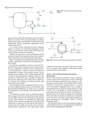
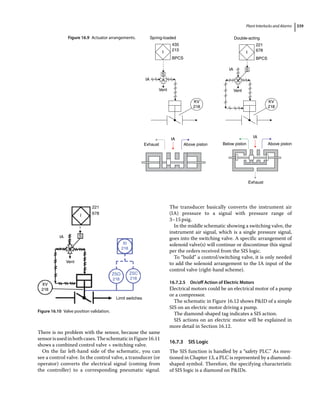
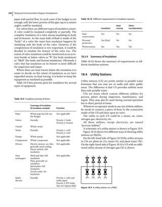
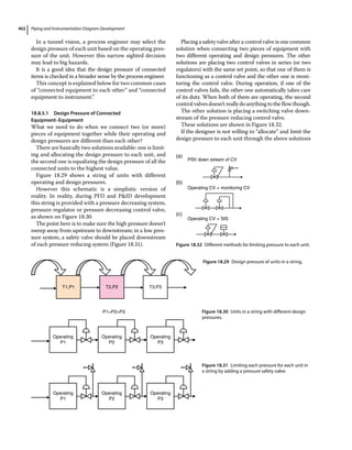
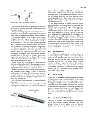
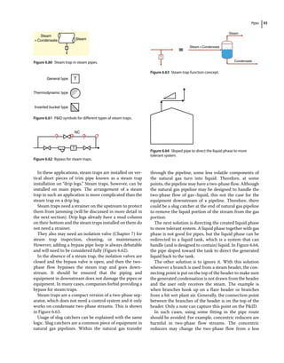
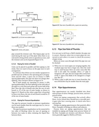
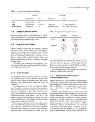
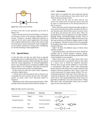
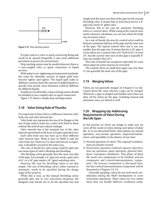
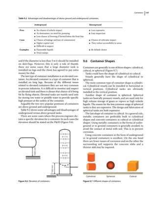
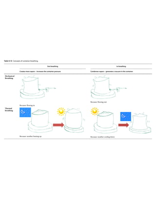
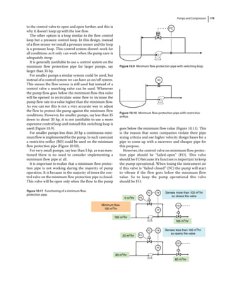
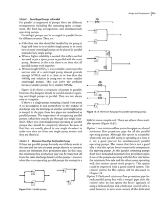
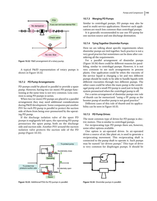
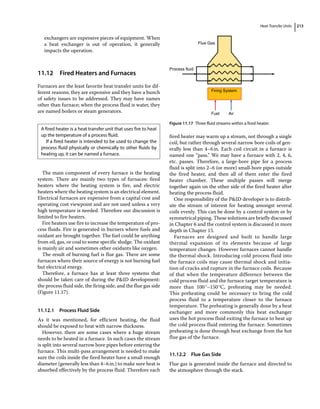
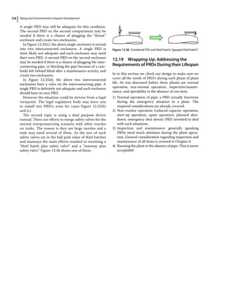
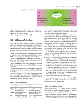
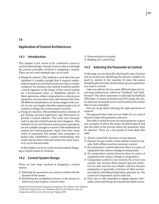
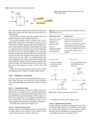
Schematics of the different types of PRDs are depicted
in Figure 12.12.
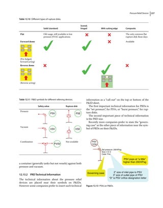
12.12.2 Rupture Disks
There are two types of non‐reclosable PRDs. In “rupture
disks,” a “hole” is covered by a disk that will rupture at a
specific pre‐set pressure, and release the pressure. The sec-
ond type of non‐reclosable PRDs is very similar to a spring‐
loaded PRV, but the spring is replaced by a “buckling/
breaking” pin. Between these two non‐reclosable PRDs,
rupture disks are more common.
Rupture disks are manufactured in main three forms:
flat, forward dome, and backward dome. These three
types of rupture disks could be in the form of a solid
sheet, a hinged or scored sheet, with a cutting edge, and
in composite. The available types of rupture disks are
shown in Table 12.10.
12.12.3 Decision General Rules
Deciding on PSD types are based on quantitative and
qualitative parameters. As many criteria go back to the
design stage of project, they are not discussed here.
12.13 ­PRD Identifiers
As it was stated in Chapter 4, the identifiers of PRDs – as
an item of instrumentation – on PIDs are PRD sym-
bols, PRD tags, and PRD technical information.
12.13.1 PRD Symbols and Tags
Table 12.11 shows P/V RD symbols and tags.
As can be seen in the table, when there is a need to
have both a pressure relief valve and a vacuum relief
valve, these two devices can be merged together to save
money on nozzles and other operating costs. The PVSV
was invented for this purpose. PVSVs (pressure/vacuum
safety valves, or as some companies call them, PVRVs
[pressure/vacuum relief valves]) are devices that protect
Inlet connection
Conventional type
Spring-type
Schematic
Dead weight-type Pilot-type
Outlet
connection
Inlet connection
Balance type
Outlet
connection
Inlet connection Inlet connection
Outlet
connection
Outlet
connection
Figure 12.12 Different types of relief valves.

245. Pressure Relief Devices 227
a container (generally tanks but not vessels) against both
pressure and vacuum.
12.13.2 PRD Technical Information
The technical information about the pressure relief
devices are placed near their symbols on PIDs.
However some companies prefer to insert such technical
information as a “call‐out” on the top or bottom of the
PID sheet.
The first important technical information for PRDs is
the “set pressure”, for PSVs, or “burst pressure,” for rup-
ture disks.
The second important piece of technical information
is the PRD size.
Recently more companies prefer to state the “govern-
ing case” as the other piece of information near the sym-
bol of PRDs on their PIDs.
Table 12.10 Different types of rupture disks.
Solid (standard)
Scored,
hinged With cutting edge Composite
Flat Old usage, still available in low
pressure HVAC applications
The only common flat
rupture disk these days
Forward dome
(Pre‐bulged,
forward acting)
Available
Reverse dome
(Reverse acting)
Table 12.11 PID symbols for different relieving devices.
Safety value Rupture disk
Pressure
PSV PSE
Vacuum
VSV VSE
Combination
PVSV
Not available PSV
1234
Governing case 2” size of inlet pipe to PSV
3” size of outlet pipe of PSV
“D” is PSV orifice designation letter
PSV pops at “a little”
higher than 200KPag
Set pressure: 200KPag
Size: 2 D 3
Case: Fire
Figure 12.13 PSVs on PIDs.

246. Piping and Instrumentation Diagram Development
228
The sample technical information of a PSV is shown in
Figure 12.13 and for a rupture disk in Figure 12.14.
12.14 ­Selecting the Right Type
of PRD Arrangement
The PSDs could be installed in different arrangements.
The simplest arrangement is a single PSD. Multiple PSDs
could be placed in some cases. They could be is series or
in parallel.
When they are in series they could be the same type or
different types. In the series arrangement it could be a
PSV and a rupture disk or two rupture disks in series.
When they are in parallel arrangement they could be
all functional (such as a 2×50% or 3×33% arrangement)
or a functional‐spare arrangement (such as the 2×100%
spare philosophy).
The parallel arrangement can also be classified based on
the similarity or dissimilarity in types. There could be mul-
tiple PSVs in parallel, or multiple rupture disks in parallel, or
few PSVs and few rupture disks in a parallel arrangement.
The different arrangements of PRDs can be seen in
Figure 12.15.
The single PSV is the default choice to protect process
enclosures (Figure 12.16). The other option is using a
single rupture disk.
However if there is a need to inspect or maintain the
PRD while the rest of the plant is operating, the PRD
needs an isolation system (isolation valve and drain/vent
valves) and some other provisions.
The provisions are the systems to allow pulling the
PRD out of operation and to allow an operator to func-
tion as a “PRD” for the time the PRD is out of operation.
There should be a connection to connect a portable
pressure gauge (or an already installed pressure gauge in
place). This system should be completed with a bypass
pipe and a manual throttling valve on it. During the time
the PRD is isolated from the to‐be‐protected system, an
operator needs to watch the pressure gauge and also be
ready to open the manual throttling valve to release the
pressure if the pressure goes higher than allowable.
Such a “manual safety system” is shown in Figure 12.17.
However not in all cases such “simple” system can be
used. The other systems to support inline care for PRD’s
will be discussed later here.
There are some cases that a single PSD doesn’t satisfy
the requirement of safety. In such cases PSDs in parallel
or in series are used.
PSDs can be placed in parallel for different reasons.
A non‐exhaustive list of cases in which we may need to
use parallel PRD’s is:
●
● When the required PRD is bigger than the maximum
available PRD in the market and several smaller PRDs
in parallel and all functioning are required.
●
● When the required PRD is big and for economical rea-
sons it is better to use several smaller PRDs in parallel
and all functioning.
●
● When there is a difference of more than 20–30% of
release flow in different credible scenarios, two (or more)
PSE
1234
Governing case
PSV pops at “a little”
higher than 200KPag
Burst pressure: 200KPag
Holder size: 2”
Case: Fire
Figure 12.14 Rupture disks on PIDs.
• Single PSD
• Multiple PSD
• In parallel
All functioning
Spare
The same type
Different type
The same type
Different type
• In series
Figure 12.15 Different PRD arrangements.
Figure 12.16 A single simple PRD.

247. Pressure Relief Devices 229
PRDs with different sizes in parallel and all functioning
should be used.
●
● When one PSV doesn’t provide the required “probabil-
ity of failure on demand” for the system two (or more)
PRDs with different sizes in parallel and all functioning
should be used.
●
● When more than one scenario is valid and each of
them calls for a different type of PSD two (or more)
PRDs with different types in parallel and all function-
ing should be used.
●
● When one PSV cannot satisfy the required reliability of
the system. In this case, again, we are going to have spar-
ing philosophies like 2×50% or 3×33% for the parallel
PRDs. The spare PSDs are used where there is a need to
inspect, recalibrate, and repair a PSD during plant oper-
ation and the “manual safety system” is not acceptable.
When there are spare PRDs each of them should have
isolation valves. The critical items are the isolations
valves upstream of each PRD. The functioning PRD
should have car seal open CSO attributes and the spare
PRD car seal close (CSC). We have to make sure that
when one upstream isolation valve is open the other
one is closed. Sometimes this is done by placing one
“change‐over valve” to make sure no mistakes happen
(Figure 12.18).
PSDs can be placed in series mainly for one reason: to
isolate the main PSD from the aggressive or dirty pro-
cess fluid. In this arrangement a rupture disk is almost
always placed upstream of (below of) the main system
protector, which could be a PSV or a rupture disk
(Figure 12.19(a)).
If there is rupture disk leakage the main purpose of the
rupture disk is missed; the connecting pipe of rupture
disk to the PSV should be “checked.”
As there is always a chance of rupture disk leakage that
the operators are unaware of the “space” should be
monitored.
The most common solution is installing a pressure
gauge on the space. A more advanced solution is install-
ing a pressure switch or pressure sensor to warn of the
increase in pressure (because of the rupture disk leakage)
to the control room (Figure 12.19(b)).
The other solution is to connect the rupture disk to a
burst sensor. The burst sensor sends a signal to the con-
trol room in the case of rupture in the rupture disk
(Figure 12.19(c)).
In Figure 12.19(d) a pressure alarm warns the opera-
tors if high pressure is created in the pipe between the
rupture disk and the safety valve.
For more severe leakages a pipe can be connected to
the rupture disk–PSV pipe. On this piece of pipe there
should be some systems. One example is placing an
excess flow valve on it (Figure 12.20).
Each of above solutions has advantages and disadvan-
tages and one may decide to use a combination of them
(Figure 12.21).
In less severe cases where the fluid is only mildly pre-
cipitating, a “flush ring” can work perfectly without the
need to go to the more complicated case of using the
combined rupture disk and PSV (Figure 12.22).
If there is a chance of contacting aggressive fluid on the
downstream of the PSV, there could be another rupture
disk installed on the PSV outlet (Figure 12.23).
CSO, FP
When relief value is functioning During relief value inspection
NC
CSO, FP Closed
Closed
Figure 12.17 A PRD with provisions for inline
care for the PRD.
CSO
2×100%
CSC
Active
2×100%
Back up
Change-over valve
Figure 12.18 2×100% spare PRDs.

248. Piping and Instrumentation Diagram Development
230
12.15 ­Deciding on an Emergency
Release Collecting Network
One important issue regarding P/VRDs is the final destina-
tion of the released fluid. An emergency release collecting
network could be used to collect the instantaneous releases
from PSDs and direct them toward the disposal system.
Figure 12.24 shows a simple schematic of an ­emergency
release collection network.
The emergency network has several requirements,
which are shown in Figure 12.25.
As is visible from Figure 12.25, the main header should
be sloped toward the disposal system. If there is needed
PG or “pressure switch to
control room
Burst sensor
PAH
SET @ 146 PSIg
(d)
(c)
(b)
(a)
123
Figure 12.19 Combination of safety valves and rupture disks.
Figure 12.20 Combination of safety valves and rupture disks.
PG
Figure 12.21 A combined solution to deal with leakage of the
rupture disk upstream of the PSV.
Utility water
Flush ring
Figure 12.22 A PSV with a flush ring.
Figure 12.23 Rupture disk upstream and downstream of a PSV on
the outlet of a PD pump.

249. Pressure Relief Devices 231
to put valve(s) anywhere on the network, such as a “root
valve”, it should be “CSO”.
The outlet of the PRDs should tie‐in from the top of
the header to make sure no liquid comes back and fill the
outlet of the PRDs.
As in the outlet size of PRDs the “no pocket” rule is appli-
cable, which means the PRDs should either be above the
header or equipped with a system to consciously or inter-
mittently drain the collected liquids from the outlet pipe of
PRDs. This system should prevent escape of gas and vapors.
To Atm.
To Safe Location
Figure 12.24 An emergency release collection network.
LR if reaction
is large
45°, 30°
or 90°
0.20–0.25%
On the top
To disposal
system
Figure 12.25 Features of an emergency release collection network.

250. Piping and Instrumentation Diagram Development
232
This system could be as simple as a one ¾″ drain hole
on the elbow (Figure 12.26) to a manual draining pot
(Figure 12.25) and to a “drip pan elbow” (Figure 12.27).
In the cases that releasing fluid may generate a huge
reaction on the piping system, it may be decided to use a
Y‐fitting instead of a T‐fitting, and long radius elbows
instead of standard elbows. This could be the case when
the releasing flow rate is huge and/or the set pressure of
the PRD is very high. Such requirements could be cap-
tured as notes on the PID.
12.16 ­Deciding on a Disposal System
The decision on the disposal system of choice depends on
different parameters. The parameters are fluid phase and
type, volume of released fluid, the governing overpressure
scenario, plant constraints, and environmental regulations.
The first thing is whether the released fluid phase is
liquid or gas/vapor.
The other parameter how “innocent” is the released
fluid? If the release gas is an air pollutant or not, if the
release liquid is flammable or not, etc.
The third parameter to consider is the volume of
released fluid. It is important to notice the released fluid
volume is different from the released flow rate. The flow
rate can be huge but if it happens in a short period of
time, the volume will be small.
A decision on the selection of disposal system is some-
times made during the PFD development stage and
sometimes during the PID stage of the project.
However, here we cover them briefly (Table 12.12).
12.16.1 Liquid Disposal
For liquid release there are different ultimate destina-
tions available; however, “system relieving” is always the
first choice. System relieving means sending the released
liquid somewhere inside of the process units. Even
though it looks like system relieving “should” be the first
choice for gas relieving too, this it is not the case. Even
though we love system relieving because the released
fluid goes back directly to the process with no wastage,
for gas release it is generally hard to find a part of the
plant that is large enough to be able to contain the
expanding high pressure gas stream.
System relieving is a common solution for PSVs on PD
pumps (Figure 12.28(a)).
The other example of liquid system relieving is in PSVs
to protect pipelines in thermal expansion scenarios
(Figure 12.29).
The next option is relieving the liquid to the sump. The
sump could be of open drain type of closed drain type
(Figure 12.28(b) and (d)).
Another option is relieving the liquid to a small bucket
(Figure 12.28(c)).
In older days it was common to spill the relieved liquid
on the ground, but these days because of environmental
regulations it is hard to do that.
3/4″ drain
hole
Figure 12.26 Preventing liquid accumulation by using a drain hole.
Figure 12.27 Preventing liquid accumulation by using a drip pan
elbow.

251. Pressure Relief Devices 233
12.16.2 Gas/Vapor Disposal
The first choice for relieving gas/vapor is disposing of it
in the atmosphere because it is the least expensive
choice!
These days this choice is allowable only if the reliving
gas/vapor is innocent.
Disposing to atmosphere is generally regulated in dif-
ferent jurisdictions. The regulatory bodies allow release
to atmosphere if the release doesn’t jeopardize the health
and safety of people and doesn’t generate pollution in the
environment.
The famous examples of releasing to atmosphere are
releasing air or steam to the environment.
Wherever it is allowed to release to atmosphere a note
is place on the PID as “to atmosphere.” The other note,
which could be confusing, is “to safe location.” Although
a PID developer may not care about the meaning of
this note, he needs to know this as there are some cases
that finding a “safe location” is not easy!
Each company may have their own interpretation of
“safe location for PRD release” and generally their inter-
pretation is outlined somewhere in their guidelines.
However, where there is no guideline the “safe location”
can be assumed as: vertical and upward release so that
the release point is higher than a minimum 3m from the
ground (or platform) and a minimum 2m from the top of
all equipment with a radius of 7.5m around the release
point(Figure 12.30).
The outlet of the PRD to atmosphere may need to be
equipped with a “bird screen” to prevent bugs and larger
animals from entering. Bird screens are tagged as an SP
item on PIDs.
Table 12.12 Ultimate destination.
Liquid Gas/vapor
●
● System relieving
●
● Open drain
●
● Closed drain
●
● Small vessel on the
ground
●
● Ground
●
● Atmosphere (if innocent)
●
● Flare (if combustible)
●
● Emergency scrubber or
quench pool (if contains absorbable
and non‐innocents)
●
● VRU (if recoverable)
●
● System relieving
(a)
(d)
(b)
(c)
PSV
Or
PSV
Figure 12.28 Different liquid disposal systems.
Pipeline
Figure 12.29 System relieving for thermal expansion PSVs on a pipeline.

252. Piping and Instrumentation Diagram Development
234
If the relieving gas/vapor is not innocent, other, more
expensive, options should be considered.
The options depend on the nature of the released gas/
vapor; if it is flammable it can be burnt in a flare; if it is
absorbable in water the stream can be sent to a catch
vessel.
Figure 12.31 shows the different available options for
gas/vapor relieving.
The last choice for gas/vapor relieving is “system
relieving.” As was mentioned before, system relieving
is not common for gases and vapors. However there
are some cases that no other option is available and
system relieving is the only technically doable option,
for example in the oil extraction industry. Well pads
are not necessarily close to the central plant, which
has a flare system. There are, however, some units
on well pads that have PRDs. Sometimes a large “pop
tank” is located to release gases from the PRDs
on the well pad. Pop tanks can be used for liquid
relieving too.
12.16.3 Two‐Phase Flow Handling
Here two‐phase flow refers to gas–liquid two‐phase flow.
We generally don’t provide a “two‐phase flow disposal
system.” What we try to do is to separate the two‐phase
flow to its components, gas and liquid, and then deal
with each of them separately.
The reason for the separation of two‐phase flow is two‐
fold. On the one hand the design and fabrication of a two‐
phase flow collection network is more complicated and
expensive. On the other hand it is not easy to find a disposal
system suitable for both liquid and gas at the same time.
However, if the liquid fraction or gas fraction of two‐
phase flow is very small, the two‐phase flow can be con-
sidered to be a single‐phase flow.
The two phase separators could as simple as Tee‐­
separators, to the more complicated options of cyclone
separators and knock‐out drums (blow‐down drums)
(Figure 12.32).
Sometimes even a combination of them is used.
To Atm.
To Safe Location
Flare Disposal
Quench/Catch Tank
Figure 12.31 Different gas/vapor disposal systems.
Min. 3 m
15m
Ground or
platform
Min. 2 m
Figure 12.30 General meaning of“safe location”for
releasing to atmosphere.

253. Pressure Relief Devices 235
12.17 ­Protecting Atmospheric
Containers
Atmospheric containers are not only atmospheric tanks,
they could be vessels that are designed with a design
pressure of less than 15psig. One example is low pres-
sure evaporators, which are used to produce potable
water from seawater. These evaporators are generally
vertical vessels but their design pressures are very close
to atmospheric pressures.
For atmospheric tanks all the overpressurizing scenar-
ios could be divided in two groups of normal over‐­
pressurizing scenarios and emergency overpressurizing
scenarios. A normal overpressurizing scenario is caused
by normal breathing of tanks when the system designed
to deal with it has failed. It is a good idea to deal with
normal breathing separated from other overpressurizing
scenarios. The reason is that it happens in almost all
types of tanks and the other reason is that the relieving
or sucking of vapors for breathing is huge.
On the other hand it was stated before that there are
two pressures that enclosures should be protected from:
internal pressure and external pressure (vacuum).
Therefore there are four components that we need to
deal with regarding tanks (Table 12.13).
Although there are four components but we don’t need
to put four separate safety valves to address them.
The atmospheric containers should be protected
against overpressure. As they are generally not designed
“full vacuum” they also need to be protected against
underpressurize or vacuum. One valve is used to cover
vacuum conditions in normal and emergency cases.
One safety valve is used to deal with emergency over-
pressurizing scenarios and one (or more) safety valves to
deal with normal overpressurizing scenarios.
The emergency valve is called a “pressure safety valve”
(tagged as PSV). This valve is to protect the tank against
emergency cases like fire.
The vacuum safety valve – for both normal and emer-
gency underpressurizing scenarios – is tagged as VSV
and the pressure safety valve for normal overpressuriz-
ing scenarios is tagged as PSV.
To save the number of nozzles on tanks, these two valves
could be combined together into one valve called a
“breather valve” or a “conservation valve” (tagged as PVRV
or PVSV), which is placed on one nozzle. The symbol of a
breather (conservation) valve is shown in Figure 12.33.
The nozzle sizes of these valves are typically 16″, 18″,
20″, or 24″.
Table 12.14 summarizes the safety valves required for
vessels and tanks.
Horizontal knock-out
drum/catch tank
Horizontal knock-out
drum with separate
catch tank
Larger pipe
size for good
separation
Cyclone
separator
Tee-separator
Figure 12.32 Emergency release two‐phase
separators.
Table 12.13 Four components of pressure issues in tanks.
Pressure Vacuum
Normal Reason Because of normal breathing; inhalation phase Because of normal breathing; exhalation phase
Extent The pressure can go as high as possible Vacuum has a limited extent, down to −101KPag
Emergency Reason Because of emergency cases like fire Because of emergency cases
Extent The pressure can go as high as possible Vacuum has a limited extent, down to −101KPag

254. Piping and Instrumentation Diagram Development
236
The other, less common, way to protect non‐pressure
vessels are “seal locks.” Seal locks are a U‐shaped pipes filled
with water (or a freeze resistance liquid) in it (Figure 12.34).
The height of the liquid column works in a similar way to a
“dead weight” in dead weight PRDs. The problem of such
PRDs is the necessity of frequent inspection of the seal lock
to make sure the liquid is in working conditions.
12.18 ­Merging PRDs
Merging PRDs can be discussed in two contexts: merg-
ing two (or more) PRDs from different enclosures and
putting a single PRD instead and merging two nozzles on
a container and using a dual purpose device instead.
Let’s start with the first topic as it is a heated topic
because it is of a technical and legal nature. In a nutshell,
the PRDs of two separate enclosures can be merged
together and only one PRD is used if there is no “obsta-
cle” between the two enclosures.
In Figure 12.35 a “story” is presented to explain this
concept. Let’s start the story from a purely technical
viewpoint (not legal).
In Figure 12.35(a), a single enclosure exists and it has
its own PRD.
In Figure 12.35(b), the above single enclosure is
turned into an enclosure with two compartments. There
is narrower enclosure between the two compartments.
Table 12.14 Two types of pressure in enclosures.
Vacuum
(external pressure)
Pressure
(internal pressure)
Schematic
Needs Vacuum protection Pressure protection
Pressure vessels PSV, mandatory Vacuum breaker
●
● No needed if the container is
designed “FV”(full vacuum)
Atmospheric tanks Emergency Normal Vacuum relief valve
Emergency vents or PSVs PRV
Could be merged as PVRV or PVSV
Pressure Valve Vacuum Valve
Figure 12.33 PVRV symbol.
Figure 12.34 Seal lock.

255. Pressure Relief Devices 237
One PRD on one enclosure
One PRD on two interconnected enclosure
Possibly one PRD in not enough and each
enclosure needs its own PRD
Definitely one PRD in not enough and each
enclosure needs its own PRD
(d)
(c)
(b)
(a)
Figure 12.35 Evolution of one enclosure to two enclosures and the concept of a PRD.

256. Piping and Instrumentation Diagram Development
238
A single PRD may still be adequate for this condition.
The second PRD on the second compartment may be
needed if there is a chance of plugging the “throat”
enclosure and create two enclosures.
In Figure 12.35(c), the above single enclosure is turned
into two interconnected enclosures. A single PRD is
most likely not adequate and each enclosure may need
their own PRD. A second PRD on the second enclosure
may be needed if there is a chance of plugging the inter-
connecting pipe, or blocking the pipe because of a care-
lessly left behind blind after a maintenance activity, and
create two enclosures.
In Figure 12.35(d), the above two interconnected
enclosures have a valve on the interconnecting pipe. A
single PRD is definitely not adequate and each enclosure
should have its own PRD.
However the situation could be stricter from a legal
viewpoint. The legal regulatory body may force you
to install two PRD’s, even for cases Figure 12.35(b)
and (c).
The second topic is using a dual purpose device
instead. There are efforts to merge safety valves for the
normal overpressurizing scenario with other nozzles
on tanks. The reason is they are large nozzles and a
tank may need several of them. As the size of such
safety valves are in the ball park value of thief hatches
and manways the main efforts resulted in inventing a
“thief hatch plus safety valve” and a “manway plus
safety valve.” Figure 12.36 shows one of them.
12.19 ­
Wrapping‐Up: Addressing the
Requirements of PRDs During their Lifespan
In in this section we check our design to make sure we
cover all the needs of PRD’s during each phase of plant
life. As was discussed before these phases are normal
operation, non‐normal operation, inspection/mainte-
nance, and operability in the absence of one item.
1) Normal operation of pipe: a PRD actually functions
during the emergency situation in a plant. The
required considerations are already covered.
2) Non‐routine operation (reduced capacity operation,
start‐up operation, upset operation, planned shut-
down, emergency shut down): PRD invented to deal
with such situations.
3) Inspection and maintenance: generally speaking
PRDs need much attention during the plant opera-
tion. General consideration regarding inspection and
maintenance of all items is covered in Chapter 8.
4) Running the plant in the absence of pipe: This is never
acceptable!
Figure 12.36 Combined PSV and thief hatch;“gauged thief hatch.”

257. 239
Piping and Instrumentation Diagram Development, First Edition. Moe Toghraei.
© 2019 John Wiley Sons, Inc. Published 2019 by John Wiley Sons, Inc.
Companion website: www.wiley.com/go/Toghraei_PID
Part III
Instrumentation and Control System
There are four “tools” that are used to control and operate
a process plant smoothly. They are the automatic control
system, safety interlock system, alarm, and mechanical
relief.
These systems help operators to run a plant. Out of
these four tools, mechanical relief was already discussed
in Chapter 12. There are three tools left to be discussed.
Before discussing the control system some preliminary
information such as terminology and symbology should
be discussed, and these are covered in Chapter 13.
Control systems are discussed in Chapters of 14 and 15.
Chapter 14 talks about important control loop archi-
tectures. Chapter 15 is a about process plant control and
has two parts: plant‐wide control and equipment‐wise
control.
Chapter 16 is devoted to safety interlock systems and
alarms. A small portion of control systems is also covered
in Chapter 16. This portion is discrete control and is
introduced in Chapter 16 because of its similarity with
safety interlock actions.
Finally, in Chapter 16, control and interlock of electric
motors are discussed as an important example.
To explain the control concepts not necessarily the
terminology of academia or even industry is used. The
goal is conveying the concepts in the simplest way.
It is important to be stated that the schematics in this
part are provided not as detailed as the rest of this book.
The schematics here are mainly to convey the concept of
control system and then some mechanical details are
ignored.

258. 241
Piping and Instrumentation Diagram Development, First Edition. Moe Toghraei.
© 2019 John Wiley Sons, Inc. Published 2019 by John Wiley Sons, Inc.
Companion website: www.wiley.com/go/Toghraei_PID
13.1 ­
What Is Process Control?
To explain a control system, we can take an example
from everyday life.
A father asks his daughter to avoid the edge of a cliff
while they are hiking. This first step is a “regulatory”
measure. A while later, the father sees his daughter playing
at the edge of the cliff; this raises an alarm and the father
tells her more harshly to be careful and step back. If the
daughter continues to play by the edge, then the father
may decide to take control of the situation; he may take
her by the hand so that they can both leave the park. These
three steps relate closely to a typical control system.
Similar to the above analogy, the first step in a process
control system is “regulation.” Regulatory control is
exercised to ensure that the process runs smoothly and
according to specifications. The more technical term for
this is a “basic process control system” (BPCS).
If the process runs out of control or off‐spec, then an
alarm is raised. This is the second step in the control
system, which alerts the operator of the need to imple-
ment stronger action to correct the situation.
If the out‐of‐control condition persists, then the control
system moves to the third step, which may involve drastic
action. In plant process control, this is called a safety
instrumented system (SIS).
So when we talk about a process control system, we
generally refer to three elements: BPCS + alarm + SIS.
Collectively, these are called an integrated control and
safety system (ICSS). We need to be specific when refer-
ring to any particular system because the general term
“process control system” may mean a BPCS to some peo-
ple and an ICSS to others.
Manipulating a plant is not limited to ICSS. ICSS is
basically “automatic control,” but we still need operators’
presence in plants. What operators do is basically
“manual control.”
They should be in the field and in the control room to
monitor parameters to take actions when they see an
emergency case.
Over the life of a plant, there will be what we can think
of as “sunny days” and “rainy days.” On sunny days, the
process runs smoothly, there is no threat to the system,
and everyone is happy. On sunny days a plant is run by a
BPCS system. Rainy days are when there is one or more
upsets in the plant. On rainy days, a plant is run by SIS
actions. SIS actions cannot be manual, but operator
intervention is provided for manual interference in
automatic SIS actions (Table 13.1).
13.2 ­
Components of Process Control
Against Violating Parameters
As was mentioned in Chapter 5 there are four steering/
protecting components for each specific process param-
eter in equipment, units, and plant.
These steering/protecting components are:
●
● BPCS. The main function of the Basic Process Control
System is to ensure that the plant runs smoothly and
within specifications. This is achieved by using control
loops to “measure” certain process parameters, “com-
pare” them to specified set points (SPs) and then
“adjust” the process accordingly.
●
● An alarm is incorporated into the system to prompt
the operator to take action when the process runs out
of control. Some people may ask why you should
bother to install an alarm when there is a backup
system, called an interlock, to deal with this situation.
If they are properly trained, the operator will be able to
make the wisest decision to override the control
system and take corrective action. This will prevent
the loss of production that would occur if drastic
action were activated via the interlock system.
●
● SIS. If a process parameter goes out of control, an
alarm is activated, which allows the plant operator to
override the system to bring the process back under
control. If he is unable to achieve this, the next layer of
control comes into play. This is the safety instrumented
system, whose main aim is to protect equipment.
13
Fundamentals of Instrumentation and Control

259. Piping and Instrumentation Diagram Development
242
At this stage, the SIS doesn’t care about process
control. It employs direct action, which may halt the
production process in order to protect the plant and its
equipment. The action of a SIS system is also called a
“trip.” The interlock system employs direct action that
will most likely halt the production process. Its main
function is to prevent equipment loss, safeguard plant
personnel, and protect the environment.
●
● Mechanical relief. If the action by the SIS is not suffi-
cient, the system moves to the last layer: relief. The
purpose of relief is not only to protect the plant and its
equipment, but also to protect the environment and
ensure the safety of plant personnel. This is usually
achieved by activating a pressure relief valve. You may
wonder why there is no relief valve for any of the other
process parameters like level, flow, and temperature.
This is because an increase in any one of these param-
eters will lead to a corresponding increase in pressure
in the plant and in the equipment. So, only a pressure
relief valve is normally needed. This concept is covered
in Chapter 12.
Here in this chapter we focus on the BPCS, alarm,
and SIS.
13.3 ­Parameters Versus Steering/
Protecting Components
The question that should be answered is whether pro-
tecting components should be placed for every single
process parameter or not. The answer is no and process
parameters should be selected for the selected ICSS
components. We are going to answer this question
regarding the BPCS and SIS. The alarm won’t be discussed
here as it is an “acting” component.
Theoretically, each element of BPCS and SIS can be
applied to each of the five process parameters: level, flow
rate, pressure, temperature and composition. So you
could have 2×5 = 10 steering/protecting loops for each
piece of equipment (Figure 13.1).
There are two other items that may potentially increase
the number of steering/protecting loops around a piece
of equipment.
One is that in addition to process parameters there
could also be non‐process parameters and the other one
is another steering/protecting loop for “only‐monitoring”
parameters.
The non‐process parameters are not as common as
process parameters. For example the torque of a rotating
scraper at the bottom of a sedimentation basin is a
non‐process parameter. Non‐process parameters, if used,
can be utilized for monitoring or interlock purposes.
More detail is provided in Chapter 16.
The monitoring parameters are the parameters that
only need monitoring by the operator in the field or in
the control room. This is different from the process
parameters we need to control and, in addition to con-
trolling them, we provide an opportunity for operators
to monitor them.
Therefore there is a “minimum” of 10 different loops
around each piece of equipment.
13.4 ­
How Many Steering Loops
Are Needed?
Placing control systems in a plant is a vital step to take
during the design of any plant. But the question that
needs to be answered is: how many control loops, alarms
and SIS actions need to be implemented in a plant? There
is no specific answer to this question. The responsible
person needs to implement the “sufficient” number of
control systems for each plant.
If the level of control is too low, you compromise the
quality of the product. The operation could also be
unsafe. The operation may lead to producing low‐quality
(off‐spec) product. The operation could be very operator
intense because of instability in the operation.
On the other hand, the larger the number of control
loops, the more system maintenance is required. If the
control loops are not well designed, they may compete
with or counteract each other. Another thing to con-
sider is that if you have installed a large number of
alarms, this can lead to operator confusion because he
is “overloaded.”
ICSS
Parameters P T
BPCS SIS
L F C
+
+
+
+
+
=
=
Figure 13.1 Swinging parameters versus steering/protecting
components.
Table 13.1 Manual versus automatic control.
Manual control
Automatic
control
Sunny days Needed BPCS
Rainy days SIS “runs the show.” Manual
control is not necessarily the
best action.
SIS

260. Fundamentals of Instrumentation and Control 243
So, a designer has to find a happy medium between
the two. The main thing to remember is not to over‐
complicate the control system.
This concept is shown in Figure 13.2.
13.5 ­ICSS System Technology
Until now, two main control “concepts” in process
plants have been introduced: BPCS and SIS. However,
each of these two concepts needs to be implemented in
the plant through “hardware systems.” Basically, carriers
are required in order to materialize these concepts in a
plant.
There are currently two main technologies that are used
as “carriers”: the so‐called distributed control system
(DCS), and the programmable logic controller (PLC).
Table 13.2 shows the three concepts of control: BPCS,
alarm, and SIS and the respective hardware systems,
which work as “carriers.”
As can be seen, the main role of the DCS is to handle
BPCS actions, whereas the role of the PLC is to handle
SIS actions.
To refresh your memory, SIS actions are on/off actions
for the purpose of safety. These may be called “safety
interlocks.”
The duty of the BPCS is to “adjust” the process to make
it run smoothly. However, the action of the BPCS is not
only regulating or throttling a valve (control valve); it
could also be opening or closing a valve!
For example, in some semi‐continuous operations you
need to close some valves and open other valves to go
from one cycle of operations to another.
One famous example is in sand filters, in water treat-
ment plants. Sand filters cannot work purely continu-
ously; they need to be pulled out of operation every so
often to be backwashed, in order to remove trapped
particles and to “rejuvenate” the filter for the next round
of operation. This BPCS action is called a “discrete
action” (as opposed to a regulatory action). Here we
need to close and open some valves (switching valves);
the intention is not safety but rather process. We call
such actions “process interlocks.”
To summarize what we have said about control sys-
tems, for each component of the ICSS, we need to decide
which technology to employ:
●
● BPCS: the control function of the BPCS can be either
regulatory or discrete. DCS technology is most often
chosen for regulatory control, through control loops.
PLCs can be employed to control single unit opera-
tions within the process, or for batch control.
●
● SIS: we can define an SIS as a set of discrete functions
for safety purposes. Here we need a very reliable sys-
tem and it has been found that a PLC is more reliable
than a DCS. For that reason, a PLC is usually selected
for this role. However, this type is not a conventional
PLC and is called a “safety PLC.”
●
● Alarm: could be run through a DCS or SIS
Now the question is: can we use a PLC for BPCS
actions, or a DCS for SIS actions? This question is
answered in the next two sections.
13.5.1 Use of PLC for a BPCS
The concept of using a DCS for a BPCS is not set in
stone. There are at least two instances where it is possible,
or even preferable, to use a PLC for BPCS actions:
1) Batch operation. A DCS is good for regulatory or
adjustmentactions.APLC,ontheotherhand,isgoodfor
discrete control that does not require adjustment – this
Low
Off-Spec. Products Low Redundancy
High Maintenance
Fighting Control Valves?
Confusing for Operators
Not Stable Operation
Not Safe Operation
Suitable
“Sweet” point
High
Figure 13.2 Level of control.
Table 13.2 Control system“carriers.”
DCS PLC
BPCS The main BPCS actions
are through the DCS
Some BPCS actions could
be through the safety PLC
Alarm Alarms through the DCS
are acceptable
Alarms through the safety
PLC are acceptable
SIS No! Not good practice to
run SIS through the DCS
All SIS actions are through
the safety PLC

261. Piping and Instrumentation Diagram Development
244
is the case for batch operations, as was mentioned
earlier. For example, in a filtration operation you have
the filtration cycle, backwash, and then filtration
again.
2) A very small plant. The DCS system was invented to
control large plants, such as a huge refinery. It is not
economical to install a DCS for a very small plant and
in this case, a PLC is preferred for process control.
Individual equipment is often supplied with a dedi-
cated PLC from the manufacturer.
13.5.2 Use of DCS for a SIS
It is not good practice to use a DCS to handle SIS func-
tions, because it is not nearly as reliable as a safety PLC.
13.5.3 Alarm Systems
The alarm system can be incorporated into the architec-
ture of either the DCS or the PLC. There are some situa-
tions where alarms (or sometimes SIS actions) are
incorporated neither into the DCS nor the PLC but
rather are hardwired. There are at least two cases where
it may be decided to hardwire an alarm (rather than
incorporate it into the DCS or PLC).
The first case is if the alarm is extremely critical and
you need to ensure that it is definitely activated, even in
the event of failure of the DCS or PLC systems. Second,
you could hardwire the alarm when the equipment is
located in a remote area where no hardware (neither
DCS nor PLC) is available.
We will talk about the symbology of alarms when we
get to alarm systems at the end of this module.
13.5.4 ICSS System Symbology
As we mentioned, there is different hardware to handle
the concepts of BPCS and SIS. When we are reading a
PID, it should be clear whether the action is handled by
the DCS system or the PLC system. Because of this, the
symbologies are different for each case.
Table 13.3 shows the typical symbology used for DCS
and PLC control systems.
A BPCS has a regulatory function via a DCS, and is
represented by a circle inside a square. The way I like to
memorize this is to equate the smooth control of a BPCS
to the roundness of a circle.
A BPCS may have a discrete function (a process
interlock). This is represented by a diamond with the
letter “I” for “interlock” inside, and the text “BPCS” on
the outside to distinguish it from a safety interlock.
It can also be shown as a diamond within a square with
“BPCS” written outside, or alternatively as an octagon
inside a square.
The main function of the SIS is as a safety interlock.
This is represented by a diamond inside a square, either
with the letter “I” or the letters “SI” inside it. It can also
be shown as a diamond inside a square with the letter “I”
in it and the description “SIS” outside. You can memo-
rize the shape of the symbol by equating its harsh action
to the sharpness and roughness of a diamond.
Using a DCS for a safety action is not good practice
and there is no symbol for that.
Figure 13.3 shows an imaginary aerial view of a plant,
showing a layer of regulatory control with a layer of
safety interlocks above it. All of the safety interlocks are
shown as diamond shapes to represent control by PLC,
Table 13.3 Example of control system symbology.
Duty DCS PLC
BPCS Regulatory
I
BPCS BPCS
H
PIC
64602
This action is named: process interlock
SIS Safety interlock
I
E SI
SIS
This action is named: safety interlock

262. Fundamentals of Instrumentation and Control 245
because very few people use a DCS for this function.
In the layer of regulatory control, the majority of shapes
are circles to show control by DCS. There are diamond
shapes here as well, to illustrate that some unit opera-
tions are controlled by PLC integrated with the DCS.
These could be equipment packages bought from manu-
facturers with their own dedicated PLCs.
In the regulatory control layer, it becomes the respon-
sibility of the IC practitioner to integrate the PLC
“islands” into the rest of the DCS.
13.6 ­ICSS Elements
Primary and final elements vary, depending on the type
of action and function of the control system, as shown in
Table 13.4.
(Primary and final elements will be discussed later but
in a nutshell, the primary element is the sensor and the
final element could be a valve or control on an electric
motor)
The BPCS is discussed in this chapter and Chapters
14 and 15. In Chapter 16 alarms and SISs will be
discussed.
13.7 ­
Basic Process Control
System (BPCS)
It is important to understand that BPCS control is not an
add‐on to a given process, but rather an integral part of
it. A good understanding of the process is essential for a
good control system.
The first question that needs to be answered is whether
we need to implement a control system for a certain
piece of equipment or not. Why should we bother to
install a control system at all?
We have to install a control system for all elements,
except for elements that meet the following three
requirements:
1) Where there is no fluctuation. In the case of a fully
closed circulating water system, for example, there is
typically no fluctuation. An example of this would be
a completely closed system, such as an HVAC system
where the flow rate doesn’t change.
2) Where fluctuation does exist, but it is not impor-
tant (i.e. it is tolerable) in the process. Sometimes
we might have fluctuation in a flow to a storage
tank – but variations in flow to a storage tank are
typically not considered important to a process. On
the other hand, a fluctuation in flow to a reactor or
a distillation tower would be a critical factor in a
process.
3) Where the equipment is self‐controlled. There are not
many pieces of equipment that are self‐controlled.
In chapter 14, various complicated loop systems are
discussed, but we don’t use these complex systems if we
don’t really need to. The best control system is a single‐
loop system.
Let’s start our discussion about control loops with a
simple daily life example of control.
Figure 13.4 shows Bill preparing to wash the dishes.
The first thing he needs to do before filling the sink is to
Safety Interlock
Regulatory Control
Figure 13.3 Imaginary layers of control.
Table 13.4 Control system elements.
BPCS SIS
Action Regulatory Process discrete Safety discrete
Name Control loop Discrete control loop SIF loop
Schematic
Primary element Sensor (sensitive toward a range) Sensor or switch (sensitive toward a point)
Final element Control valve or
VSD on electric motor
Switching valve or
start‐up/shutdown switch on electric motor

263. Piping and Instrumentation Diagram Development
246
set the tap temperature. The following is the sequence
of steps for doing this:
1) Bill’s left hand (the “sensor”) monitors the temperature
of the water coming out of the tap.
The sensor sends a temperature signal to Bill’s brain
(the “controller”). The controller contains in its regis-
try a “set point” of 35°C, a comfortable temperature
for washing dishes.
2) The controller checks the reported temperature
against its SP.
3) The controller sends a temperature adjustment signal
to the control valve.
4) The control valve interprets the signal and adjusts the
hot or cold water flow required to achieve a dishwater
temperature of 35°C.
In this example, the “control valve” is the lever on the
hot and cold water mixer tap. The “actuator” for the
control valve is Bill’s right hand. The actuator adjusts the
control valve upon receiving a signal from the controller,
based on a SP that resides in the controller.
Now we want to show the above control loop with the
symbology used in PIDs (Figure 13.5).
We need to start with defining the devices involved in
the control loop:
●
● TE: temperature element, or sensor
●
● TT: temperature transmitter
●
● TC: temperature controller
●
● TV: temperature control valve (the acronym is not
TCV!).
Using the above definitions, we can outline the sequence
depicted Figure 13.6. Note that it is assumed that the
tap has been opened before step 1 of the sequence:
1) The TE records the tap water temperature.
2) The TT transmits this value to the TC. The transmis-
sion is represented by the dotted line.
3) The TC compares the received value against its regis-
tered SP.
4) TheTCsendsatemperatureadjustmentsignaltotheTV.
5) The TV adjusts the flow of hot and cold water.
All control loops include transmitters, whether they
deal with temperature, pressure, level or flow. However,
not all companies show transmitters on their PIDs. The
reason is that transmitters are essentially signal channels
with no “process” duties, and some companies prefer not
to show non‐process items on their PIDs. The purpose
of the transmitter is to convert the signal created by the
sensor into a signal that is “good,” i.e. clear and strong
enough to reach the controller, which is usually located
in the control room.
All of the elements in one control loop need to have a
single unique sequence number. In Figure 13.6, this
Set point
Control Valve
Sensor
Controller
I want 35°C
Figure 13.4 Everyday example of a control loop.
TT
123
TE
123
TV
123
TC
123
Figure 13.5 Temperature control loop.

264. Fundamentals of Instrumentation and Control 247
number is 1001. Sometimes the elements of a single
control loop do not all appear on the same PID sheet,
so if these elements have all been assigned the same
sequence number, we can still find them easily in different
PID sheets.
Now, we will continue to look at the second example of
a simple level control loop.
Figure 13.6 illustrates fluid level control in a tank,
rather than fluid temperature control.
The devices in this loop are defined as follows:
●
● LE: level element, or sensor
●
● LT: level transmitter
●
● LC: level controller
●
● LV: level control valve.
There is no “LE” in Figure 13.7 and nothing is missed
there! There are some cases that there is no specific sen-
sor for a process parameter and the signal is initially
developed in the transmitter, which is “LT” here.
For level measurement, there are two types of sensor:
contact sensors and roof sensors.
Contact level sensors are the most famous sensors in
that their signal is developed in their transmitter and no
“LE” exists for them.
Using the above definitions, we can outline the
sequence depicted in Figure 13.6:
1) The LT transmits the level value in the tank, as
measured by the contact sensor, to the LC. The
transmission is represented by the dashed line.
2) The LC compares the received value against its regis-
tered SP.
3) The LC sends a level adjustment signal to the LV.
4) The LV adjusts the control valve to modify the
outflow from the tank in accordance with the
instructions received from the LC.
For example, let us assume the SP to be 2m. This
means the level needs to be constantly adjusted to 2m
from the bottom of the tank. If the level is reported at
2.5m, the LC compares this value against the 2m SP and
recognizes that the tank contains an average of 0.5m
more than the SP. Therefore, the LC sends a signal to the
LV to adjust the level downward by opening the valve to
increase the outflow from the tank.
This example illustrates that each control loop has
three functions: measuring, comparing, and adjusting.
13.8 ­Instruments on PIDs
A piping and instrumentation diagram (PID) is a sche-
matic drawing used to illustrate all of the elements used
in the control of a process. It is a diagram that shows how
all the pieces of process equipment are interconnected,
together with the instrumentation used to control the
process. Symbols used for both equipment and instru-
mentation conform to the global guidelines given by the
ISA, the International Society of Automation.
13.8.1 Fundamental Terminology
I would like to explain some fundamental terms that
are used in process control, specifically relating to
­
control loops (Figure 13.7). First, you have a primary
element (sensor), which is usually an instrument that
measures a process variable. A signal is sent via a
transmitter to a controller. The controller then sends
an adjustment signal to the final element.
The final element is some mechanical means to ­control
the process. This is often a control valve on a pipe, or a
variable speed drive for a pump or compressor.
13.8.2 Identifiers for Equipment
and Instrumentation
Here we want to learn the identifiers of instruments.
We will start our discussion with a table that compares
equipment versus instrument identifiers.
1 Measure
3 Adjust
LC
1001
Set point
LT
1001
LV
1001
2 Compare ⤍ to set pont
Figure 13.6 Level control loop.
Primary element
Final element
Instruments
Signals
FT
215
FE
215
FC
215
FV
215
Figure 13.7 Fundamental terminology.

265. Piping and Instrumentation Diagram Development
248
Table 13.5 gives examples of the typical identifiers
that are used for both equipment and instruments. The
identifiers used for equipment are different to those
used for instrumentation.
For equipment, we use the actual shape as a symbol;
there is a different one for each type of equipment. Each
piece of equipment has an identifying tag and a call‐out,
which gives key information about the operating param-
eters of the equipment. The call‐out information can be
inserted at the top or the bottom of the PID.
On the other hand, instrument symbols don’t resemble
the actual shape of the instruments. They specify the
function and the location of the instrument. Instrument
symbols (or “balloons”) generally conform to ISA
specifications.
For instruments, we do not use a call‐out. A tag is used
to describe the function of the instrument and is between
two and four letters long.
13.9 ­Instrument Identifiers
When we show an instrument on a PID, there are five
items that we need to specify (Figure 13.8):
1) Acronym
2) Divider type
3) Symbol type
4) Additional information
5) Tag number.
We will discuss all of the identifiers except the last one
(tag number). The tag number is simply a sequence num-
ber for an instrument. A big help when reading a PID is
that all the elements in one control loop have the same tag
number. This fact helps us to find different elements of
one control loop when they are on different PID sheets.
13.9.1 Acronyms
Acronyms are composed of two “bags”; one left hand
bag and one right hand bag, as shown in the schematic
in Figure 13.9. Each “bag” may have one or two letters.
The second letter of each “bag” is not mandatory.
Therefore, we can say that an instrument’s acronym can
have between one and four letters.
The meaning of each letter in the tag’s acronym is
presented in Figure 13.9.
The first letter is mandatory and is used to describe the
process parameter that is being controlled. Most of the
first letters of the acronym are self‐explanatory, except
“A.” “A” represents composition, based on the word “ana-
lyte,” which is the word used by chemists and lab techni-
cians for any composition parameter being measured.
The second letter is called a “process parameter
modifier.” This is an optional parameter, and we use it
Table 13.5 Instrument identifiers.
Equipment Instruments
Example T-1325
T-1325
2.2 KPag @80C
FIC
123
Call‐out
Tag Two to four (or more) letter
and
tag number
Symbol Different for
different
equipment
For sensors: different
symbols for different
Sensors
For the rest of instruments:
different balloon shapes
Symbol
represent:
Actual shape of
equipment
Function of instrument and
the location of instrument
1st Letter
2nd Letter
L Level
T Temperature
E Element (sensor)
T Transmitter
C Controller
I Indicator
L Low
LL Low Low
H High
HH High High
F Flow
P Pressure
A Composistion
D Differential
Q Total
F Ratio (Fraction)
1051
Succeeding Letters - 1
Succeeding Letters - 2
Figure 13.9 Acronym descriptors.
1. Acronym 4. Additional info.
5. Tag No.
A/B
FY
123
2. Divider type
3. Symbol type
Figure 13.8 Instrument identifiers.

266. Fundamentals of Instrumentation and Control 249
when the process parameter of interest is not a simple
parameter. In other words, it involves some computational
aspect of the parameter, e.g. ratio, total or differential.
For instance, “PD” would indicate the measurement of
a pressure differential between two points in the process.
The use of PD is of great benefit wherever flow goes
through an obstructed route like in filters, strainers or
even ion exchangers. The PD is used to ascertain when
the porous medium has become plugged and needs
backwashing. The modifier of “D” is widely used for
pressure but it is not common for other parameters.
Another example is the use of “Q.” “F” means flow
rate, but “FQ” means volume (total of flow rates means
volume!). The modifier of “Q” is used arguable only for
flow rate as it is not generally meaningful for other
parameters. The total flow rate could be important for
some utility streams, on some intermittent flow pipes,
or other cases.
The use of the ratio descriptor is very useful for
flow, and the acronym for this would read “FF.” This is
of particular importance in dosing systems, where you
need to control the dosing rate according to the flow
rate of the process stream.
The third letter is called the function letter, which is
what we want to do with the parameter obtained and
mentioned in the parameter of choice stated in the first
letter. If the instrument is sensor, we use the letter
“E”(element); if it is a controller, we use “C,” etc.
If the instrument is an indicator, we use the letter “I”
but usage of “I” is not as common as in older days. The
reason will be discussed in Section 13.9.3.
The fourth letter in the acronym is, again, an optional
descriptor. The fourth letter is a modifier that is most
often used for alarm purposes or in SIS actions to indi-
cate the action point of a loop, for example, high, low
or low‐low.
Table 13.6 gives more examples of instrument
acronyms.
Figure13.10givesonecompleteexampleofacontrolloop.
13.9.2 Divider Types
The balloon dividers generally specify the “location” of
instruments. What is important from an IC practition-
er’s viewpoint regarding “location” is if the instrument is
in the field, in the control room, or in the field cabinets.
Different divider shapes are shown in Table 13.7.
In Table 13.7, I have shown the symbol with an irreg-
ular shape. This is so that you focus on the divider and
not the shape. The shape of the symbol will be discussed
in Section 13.9.3.
For the divider, there are five different cases:
1) No divider. This means that the instrument is out-
doors, in the field. Examples are a flow element or
sensor, or a level switch or gauge. They are connected
to the control system, but they are not encased in a
control room or in an auxiliary control cabinet. The
majority of sensors are located outdoors and their tag
doesn’t have any divider.
2) Single solid line . This shows that the instrument
is situated inside the main control room. It also indi-
cates that the instrument is accessible and visible to
the operator.
Table 13.6 Examples of instrument acronyms.
No. Examples
What is the parameter we
are looking for?
What we want to do
with the parameter?
Meaning
Parameter of
interest
Parameter
modifier Function
Function
modifier
Example 1 FQI F Q C Volume of fluid is controlled
Example 2 LT L T Liquid level is transmitted
Example 3 TC T C Temperature is controlled
Example 4 PDC P D I Pressure difference is shown
Example 5 AT A T An analyte is transmitted
Example 6 LEHH L E HH Level sensor alarms on “HH” level
LC
504
FT
504
Loop No.
Loop No.
Loop No.
Loop No.
FE
504
LV
504
Flow Indicator Controller
Flow Control Valve
Flow Transmitter
Flow Element
Figure 13.10 Instrument acronyms shown on a PID.

267. Piping and Instrumentation Diagram Development
250
3) Single dashed line . This shows that the instru-
ment is located inside the main control room, but it is
not that important and is inaccessible to the operator.
In the past, before computerized control, instruments
were mounted on a board in the control room. The
important ones were mounted on the front of the
board and those that were deemed less important
were mounted on the back of the board. So, this is the
same concept.
4) Double solid line . This indicates that the instru-
ment is situated in a control cabinet in the field and
is accessible and visible to the operator. Dedicated
control cabinets are supplied by manufacturers, espe-
cially for PLC control of their equipment.
5) Double dashed line . This means that the instru-
ment is in a field control cabinet, but inaccessible to
the operator.
The meanings of different dividers are summarized in
Figure 13.11.
13.9.3 Symbol Type
We talked about this previously in this chapter. There are
three different types of symbols for instruments, as
shown in Figure 13.8.
The three types you see represented are:
1) A circle on its own. This represents an instrument
that gives a measurement or readout. It has no con-
trolling function, i.e. it has no brain.
2) A circle within a square. The square shows that the
instrument has some controlling function. The
­
circle represents a smooth control process, such as
a DCS.
3) A diamond within a square. Once again, this instru-
ment has a controlling function. The diamond indi-
cates that the control process is via a tougher system
like a PLC. This type is also sometimes shown as an
octagon within a square.
The way that you can memorize these cases is this
statement:
“no divider; no enclosure,”the rest are in enclosures.
Table 13.7 Divider types.
Location
Unenclosed location Enclosed locations
In field
In control room In field cabinet
In accessible location
In inaccessible
location In accessible location In inaccessible location
Symbol
(divider
type)
Examples All sensors, all
transmitters
Controllers,
indicators
Non‐important
functions
Local alarms Transducers
Why do we use dashed lines?
In this symbology, we use dashed lines based on the
interpretation we borrowed from drafters. Did you know
that drafters draw hidden lines as dashed lines? We use
the same concept here. The items are behind a board are
invisible and we show them with a dashed line.
Field Control Room
Figure 13.11 Instrument divider types versus their location in
reality.
The way that I memorize this is:
A single symbol means “no brain.” A double symbol
means“a brain”is involved.
This has a circle with a soft and round perimeter,
similar to the soft DCS system.
This has a diamond with sharp, tough corners,
similar to the tough SIS system.

268. Fundamentals of Instrumentation and Control 251
It is important to note that we show symbols like or
not only when they have a “brain” (controller), but also
when a piece of data can be seen through the monitor
connected to the control system. This justifies symbols
like this ; it is not a brain, it is only an indicator, but we
use a circle to show it is visible through a DCS monitor.
By combination of Tables 13.7 and 13.8 we can see the
famous table of instrument symbology that you may
have seen several times on the first sheet of a set of
PIDs (Table 13.9).
Table 13.9 is a table that was originally developed by
the ISA and is well known in the control and instrumen-
tation industry. It shows the types of symbols used for
instruments in different locations.
With current technology there are some symbols that
are no longer common. The reasons are as below:
●
● Field‐mounted items: “discrete instrument” means an
instrument with no controlling function. These are basi-
cally sensors and transmitters. As we know, sensors are
installed on processes, which are located in the field (i.e.
not inside the control room or a field cabinet).
Transmitters are connected to sensors and as close as
possible to them. That is why they generally don’t have
any divider for sensor and transmitter symbols. It doesn’t
make sense to install a sensor or transmitter inside a
control room or inside a field cabinet. Therefore, it is rare
to see any type of divider for a sensor or transmitter.
●
● “Brains,” either DCS or PLC, are too delicate to be
installed in the harsh environment of the field.
Therefore, there is no “square”‐type balloon, with no
divider. DCS and PLC systems are generally installed
indoors, so they have some sort of divider.
Table 13.8 Types of instrument symbols.
Symbol
(balloon type)
Non‐technical
definition Example
Whatever has no brain Sensors, transmitter
Brain in DCS
and
whatever can be “seen”
in DCS monitors
Whatever other than
above! But not part
of SIS
Brain in PLC The logic holder in
SIS loop
Table 13.9 Instrument symbology.
Non‐technical definition
Unenclosed
location Enclosed locations
In field
In control room In field cabinet
In accessible
location
In inaccessible
location
In accessible
location
In inaccessible
location
Whatever has no brain
Common
Brain in DCS
and
whatever can be “seen”
in DCS monitors
Common Common
Brain in PLC
Common Common Common

269. Piping and Instrumentation Diagram Development
252
●
● Back‐of‐panel items: there is no such thing as “back‐of‐
panel” in today’s control rooms. In the old days there was
a real panel in control rooms and some not very impor-
tant instruments could be checked and monitored only
by going to the back of the panel. However, these days all
the panels in control rooms have been replaced with
monitors, thus there is no panel of a back of panel. So, a
single dashed line, , is very rare.
However, we still have backs‐of‐panels for field
cabinets, i.e. .
13.9.4 Additional Information
and Tag Number
There are no set rules as to where to put additional
information about the instrument on a PID. However,
usually you place it at the top right or bottom, right next
to the symbol, as shown in Figure 13.12.
There are at least three different instances where you
need additional information for the instrument in
question:
1) For function clarification
2) For carrier clarification
3) For tag clarification.
●
● Function clarification. Different examples are
shown in Figure 13.12(a). Generally speaking, how-
ever, wherever there is a non‐defined letter in an
instrument symbol, it needs to be specified outside
of the symbol.
To explain further the concept of a “non‐defined”
letter we need to refer to table 4.1 of ISA standard
ANSI/ISA‐5.1. The non‐defined letter could be a
“user’s choice” letter (like “M”), or an “unclassified
letter (like X)”, or letters that refer to general actions
(like “Y” or “U”), which are not precisely defined.
In the first example we see “FY”; “Y” is a
­
mathematical operator that is applied to a flow, “F.”
The question is, “what is Y?” We have specified it
outside and put the symbol “,” which means
“larger than.” This means that this balloon receives
more than one flow signal, and this balloon will
pick the largest flow rate.
Another example is a UA balloon. “A” is alarm
but “U” is a wildcard letter and needs to be speci-
fied; outside of the symbol it says that “U” refers to
any problem in the system, or “common alarm.”
The last two examples are interesting because
the letters used in symbols are clearly defined by
the PID developer deciding to “clarify” them out-
side of the symbols.
Another example is PI. This example is different
than the previous ones. Here there is no wildcard
or unknown parameter. However, some people
could be confused about the purpose of measuring
and indicating pressure in that specific application.
In that case, the designer would explain that “we
are measuring the pressure to make sure there is no
leak from the system.”
Yet another example (not shown here) is a com-
position element, AE. In this case, you need clarifi-
cation by showing what analysis is being conducted,
e.g. pH or H2S in gas, because “A” doesn’t tell us
what the analyte is.
●
● Carrier clarification. As shown in Figure 13.12(b),
we can clarify the carrier, or type of control system,
that the instrument relates to. This is written on
the bottom right‐hand side of the tag and can be
“BPCS,” “SIS” or “BMS.”
A “BMS” is a “burner management system.” This
is essentially an SIS that is a critical and mandatory
part of burner management in industry. In some
jurisdictions BMS is mandatory when you deal
with a fired system.
●
● Tag clarification. In Figure 13.12(c) we show an
example of a tag for a flow controller, FC, which is the
same for two different items, A and B. To clarify this,
we show the lettering A/B on the side of the symbol.
The other example shows an interlock, or “I.” This
has the number 1091 written on the side. The num-
ber 1091 relates to the action that would be taken by
the SIS. You would have to refer to the cause and
effect diagram, or shutdown key, to see what action
would be taken when SIS loop 1091 is activated.
13.10 ­Signals: Communication
Between Instruments
Communication between control instruments is via dif-
ferent types of signals. We need to have a look at how this
is shown on PIDs (Figure 13.13).
(a) Function Clarification
(b) Carrier Clarification
(c) Tag Clarification
FY
123
UA
439
PI
200
FC
592
FC
592
FC I
592
BMS BPCS
COMMON ALARM LEAK
1091
A/B
Figure 13.12 Additional information.

270. Fundamentals of Instrumentation and Control 253
If the two elements are situated within one housing, we
show them side by side with no evidence of a signal
(Figure 13.13(a)). In reality, you need something to carry
a signal between the two but this is obviously part of the
internal wiring of the particular control panel. If the two
instruments are situated in remote locations, you need to
show a signal line connecting them (Figure 13.13(b)).
13.10.1 Signal Types
There are different types of signals that are used for
communication in process control instrumentation
Table 13.10).
●
● Capillary line . A capillary line is a
tube with trapped innocent liquid. This tube is used
when we try to “transfer” the process fluid to an instru-
ment without sending the process fluid inside of the
instrument, possibly because the process fluid is non‐
innocent. This is primarily used for sensors in some
special cases.
●
● Electrical signal . An electrical signal can
be either analog or digital. This has traditionally been
an analog signal, but the latest technology is moving
more toward the digital form. Although there is a
difference in an analog‐electrical signal versus a
digital‐electrical signal, we can consider
as the general symbol for electrical signals, whether
analog or digital. Electric signals can be considered
as the “default” signal in today’s process plants.
●
● Pneumatic signal . The majority of control
valves are actuated by pneumatic signals. The pneu-
matic signal is generally provided by “instrument air”
(IA). However, other gases could be used if IA is not
available. This type of signal is used for the majority of
control valves and switching valves.
●
● Hydraulic signal . In some cases, hydraulic
actuation is necessary for the operation of a control
valve or switching valve. First, in a remote location
like an oilrig, an instrument air facility may not be
available. Second, if the pressure in a pipe is very high
and the instrument air pressure will not be able to
adjust the valve, then hydraulic oil is needed to open
and close the valve. In such cases, a hydraulic oil pack-
age needs to be purchased, instead of an instrument
air package.
●
● Software signal . Software signals are
actually computerized signals. The simplest form of a
software signal may be established by an RS‐232 cable,
which is very famous in the computer industry. In
plain English, a software signal is a digital signal
whereby digits are sent in a specific pocket size and a
specific time/duration. These signals are sent where
two controllers (balloons with “C” in them) want to
communicate with each other.
There are some companies who put arrows on their
signals and there are other companies that don’t follow
this practice. In either case, to correctly interpret a
control loop, the PID reader should put arrows on the
signals in his mind, even where they don’t exist.
Now the question is what we need where a signal
extends beyond a PID sheet. The answer comes with
the same logic of pipe extension: off‐page connectors.
Figure 13.14 shows off‐page connectors for a signal.
13.10.2 Signal Functions
Signal functions are drawn as balloons that process
signals to convert them to other types of signals. There
are two main categories of signal functions: signal math
FIC
(a)
(b)
256
FIC
200
FIT
1051
FI
1051
Figure 13.13 How do“boxes”communicate?
Destination PID no.
Destination Instrument
To FY-328
PID-52-1708
Signal
Signal name
Figure 13.14 A leaving off‐page connector for a signal.
Table 13.10 Types of signals.
Signal symbol Signal name Common application
Capillary tube To some fluid‐in
sensors
Electrical‐
analog signal
By default choice
Electrical‐
digital signal
Advanced choice
Pneumatic
signal
On pneumatic
control valves that
are very common
Hydraulic
signal
On hydraulic control
valves
Software link Connection between
“brains”

271. Piping and Instrumentation Diagram Development
254
functions and signal selectors. We will explore these two
in the following two subsections.
13.10.3 Signal Math Functions
Signals are not always straightforward and sometimes
we want to add them, multiply them, divide them, and
also use the difference between them to create a new
control signal.
There are control applications where we need to use a
function curve, f(x). For example, when you need to con-
trol the pH of a stream/liquid inside a vessel, the control
will be based on a titration curve. The titration curve is
digitized to form a function curve, which is then used to
control a neutralization system.
Some of the most common math functions are listed in
Table 13.11.
13.10.4 Signal Selectors
In some instances, we have more than one signal availa-
ble for control, and we need to select one of them.
Table 13.12 shows the various options that are most
often used for signal selection. In the next chapter you
will see some application of these signal selectors.
Figure 13.15 gives examples of how signal selectors
work. These are quite self‐explanatory for each case.
Limiting selectors have an internal “constraint.”
It is good to know that a “magnitude limiter” is the
same as a “magnitude selector” when the magnitude
selector function is constrained with a constant value
rather than another signal (Figure 13.16).
You might assume that in order to make a selection,
the signals need to be homogenous, i.e. both must come
from a flow sensor or temperature sensor, etc. This is not
always the case; the signal selector does not care where
the signals come from – they only look at the value
assigned to each signal in order to make a selection.
Figure 13.17 gives an example of a non‐homogenous sig-
nal selection scenario.
In the cases of non‐homogeneous signal selectors the
problem is how to tag the selector. If two signals are flow
signals the selector can easily be tagged as “FY” and if
Table 13.11 Signal math functions.
Signal symbol Signal name Meaning
+
Σ
Summing Adding two signals together
–
∆
Subtracting Subtracting one signal from
other signal
±
Bias Subtracting one signal from a
constant value
x
Multiplying Multiplying two signals
together
k
Proportional Multiplying one signal to a
constant value
÷
Dividing Dividing two signals
Σ/n Averaging Averaging several signals
√
Root
extraction
Measuring the root of a signal
f(x)
Function Applying a complex function
on a signal
d/dt
Rate Measuring the rate of a signal
Table 13.12 Signal selectors.
Symbol Selector name Function
High selector Picks the higher magnitude signal
Low selector Picks the lower magnitude signal
|
High limiter Picks the higher magnitude signal
up to certain value pre‐set for it
|
Low limiter Picks the lower magnitude signal
down to certain value pre‐set for it
HS
(Soft) hand
switch
Picks a signal based on the operator
intent
FY FY
7
7
8 8
7
8
8 8
8
4
8
8
7
7
10 10
10
10
FY
FY
FY FY
Figure 13.15 Examples of signal selection.
FY
8
Constraint:8
FY
Figure 13.16 Magnitude limiter and magnitude selector.

272. Fundamentals of Instrumentation and Control 255
two signals are temperature signals the selector can
easily be tagged as “TY.” Some companies drop the first
letter and some other companies only show the higher or
lower sign instead of showing the whole symbol.
There are some signal selectors that are specifically
used for discrete signals. These are mainly permissive
operators, and inhibitive operators.
The meaning of them is shown in Figure 13.18.
Although I show the meaning of these two functions
schematically, on PIDs generally they are not shown.
The permissive and inhibitive functions are generally
captured on PIDs only by notes.
●
● Permissive. The selector will only send an outgoing
signal if both incoming signals are present, i.e. assigned
a “1.” If one of the signals is absent (a “0”), then the
selector does not forward a signal. This function is
used in applications where one action needs to be
performed in order to activate the other action. For
example, an operator pushbutton for shutting down a
centrifuge may have a permissive function of the open
wash water valve. In this example, pushing the shut-
down button of the centrifuge doesn’t work unless the
system is already being washed by water through the
opening of the wash water stream.
●
● Inhibitive. This selector works in the opposite way to
the permissive selector. This means that if there are
signals from both incoming sources, the selector will
not produce an outgoing signal. Only if either of the
incoming signals is absent will the selector send a
signal.
13.11 ­
Different Instrument Elements
In this section the main elements of a control loop are
discussed. They are primary elements (sensors), trans-
mitters, controllers, indicators, and the final elements.
13.11.1 Primary Instruments
There are three main types of primary elements. They
are sensors, gauges, and “gauge points.”
Sensors and gauges, both, have sensing components
and both of them are used to measure process param-
eters, but the former generates a signal (e.g. electric
signal) proportional to the magnitude of the process
parameter while the latter does not. This shows their
applications; gauges are installed when the intent is to
show a process parameter in the field to the rounding
operator, whereas an element’s reading can be seen in
the field and in the control room. Therefore a field
gauge cannot be part of the control system.
“Gauge points” are nothing except a “point” that is
“planted” somewhere on the plant to be used by an
operator to check the process (or non‐process) param-
eter with his portable gauge.
From this, you can deduce that gauges and sensor
point never ever connected to other instruments on
PIDs.
All the primary instruments are installed in field then
they don’t have any divider in their symbols.
Table 13.13 shows a list of gauges.
Elements have a more complicated structure than
gauges. Gauges are not very complicated. For example, a
temperature gauge (TG) could be a bimetal, wherein
dissimilar expansion of an attached metallic ribbon
causes its deviation and movement.
FGs are nothing more than a piece of transparent pipe
that can be installed along a portion of piping. FGs are
named “flow sight glasses.” The FG gives the operator a
visual indication of flow.
The PID symbol for a sight glass can be as shown in
Figure 13.19.
FY
Acceptable
Represent: T
Represent: F
Or T?
Figure 13.17 Signal selector on non‐homogeneous signals.
Y
1 1
1
Y
1 0
0
Y
1
Inhibitive
Permissive
Discrete Signal Logical Functions
0
1
Y
1 1
0
Figure 13.18 Discrete signal logic functions.
Table 13.13 Gauges.
Parameter T P L F A
Tag TG PG LG FG Not available
SG
Figure 13.19 Flow sight glass.

273. Piping and Instrumentation Diagram Development
256
Measuring process parameters is uniquely done by
“process analyzers,” or “AEs.” They are too complicated
to be built in the form of AG or gauge.
However there are some gauges than can be connected
to indicators too.
Table 13.14 shows a list of sensors.
Some companies use acronym for gauges instead of
elements interchangeably.
The portable gauges need specific locations on the
plant to be able to “cling” on to them to measure the
parameters. These “sensor locations” should be tagged
on the PIDs. A list of them is given in Table 13.15.
It can be seen from the table that gauge points are
generally limited to pressure points and temperature
points, or thermowells.
Some companies, instead of the acronym “PP”, use
“PT”, which means “pressure tap.”
Now we are going to give a brief review of primary
elements or sensors. It is important to stress that this is
only a “summary” for the purpose of PID development.
There is a huge amount of knowledge regarding sensors
and the selection of them for different applications is
beyond the scope of this book.
In this section we talk about each of five sensors, tem-
perature sensors, pressure sensors, level sensors, flow
meters, and process analyzers. For each of them we
briefly talk about each group and the common types of
sensors. Then the different methods of connecting sen-
sors to process items are shown. These methods are
known as “hook up” arrangements. The hook up arrange-
ments are not always shown on PIDs, but it doesn’t
mean they don’t exist. Some companies prefer to not
showing them just to avoid crowdedness on PIDs.
The PID symbol for each of the sensors is introduced
heretoo.However,sometimes,especiallyintheearlystages
of PID development, the exact type of a sensor is not yet
decided. In such cases just the tag of the sensor may be
used as its symbol. Obviously this should be replaced later
with the exact symbol of the selected sensor.
13.11.1.1 Temperature Measurement
Temperature measurement can be done everywhere on
flow of gas, liquid, or flowable solids.
It also can be done for parts of equipment. One exam-
ple is “skin temperature,” which is the temperature of
the coil wall inside fired heaters. The other example is
measuring the temperature of winding in high power
electric motors.
A unique feature of temperature measurement is that
they are types of sensors that work remotely. For exam-
ple the temperature a flue gas stream can be measured
remotely.
Temperature sensors generally don’t have any specific
symbol on PIDs.
Table 13.16 is a non‐exhaustive list of common tem-
perature sensors.
Table 13.14 Sensors.
Parameter T P L F A
Tag TE PE LE FE AE
Table 13.15 Gauge points.
Parameter T P L F A
Tag TW PP Not generally needed Not generally needed Not available
Table 13.16 Temperature sensors.
Type Unique advantage Unique disadvantage Application
Thermocouple Default choice for wide
temperature range
Sensitive to noise Specially in burner management
system (refer to Chapter 16)
Resistance
temperature detectors
(RTD)
Very accurate Needs power source Process pipeline temperature
measurement
Thermistor High accuracy ●
● The narrow range
●
● The most inexpensive
temperature sensor
More in laboratory but not in
industrial process control.
Infrared Non‐contact type Needs line of sight Common for remote temperature
sensing in combustion systems

274. Fundamentals of Instrumentation and Control 257
Temperature sensor arrangements: when the pipe size
is small it is not easy to place a thermocouple in it.
“Small” is defined differently in different companies.
Some companies consider small to be sizes smaller than
4″ but some other companies consider 3″ or even 6″.
There are two solutions when faced with the issue of
placing a thermocouple in small size pipes. One is using
a combination of enlarger–reducer to enlarge the pipe
size and then placing the thermocouple (Figure 13.20).
The other solution is placing the thermocouple on a
bend of the pipe (Figure 13.21).
If the purpose of temperature measurement is skin
temperature, it could be mentioned beside the balloon
on the PID, or showing the connection to the surface.
Figure 13.22 shows a PID with both of them together.
13.11.1.2 Pressure Measurement
Pressure measurement can be done everywhere on the
flow of gases or liquids.
However, measuring the pressure of liquids is not as
common as gases and vapors.
Temperature sensors generally don’t have any specific
symbol for PIDs.
Table 13.17 is a non‐exhaustive list of common pres-
sure sensors.
Pressure sensor arrangements: some companies shows
PGs and PIs simply as in Figure 13.23.
However, this doesn’t necessary mean that there is
nothing between the gauge and the process. There are
generally different items on the connecting tube.
As a minimum there should be one isolating valve – a
root valve – and a drain/calibration valve (Figure 13.24).
In some critical cases, instead of one root valve, two
root valves and a drain can be placed (Figure 13.25).
In the cases where the process fluid is harmful to the
internal parts of the sensor, a diaphragm can be placed
and the space between the diaphragm and the sensor
TE
2″ 2″
Figure 13.20 Thermocouple installation on narrow pipes (option 1).
TT
123
TE
123
SKIN
Figure 13.22 Skin temperature sensor.
2″
2″
TE
Note 1
Note 1:On pipe elbow
Figure 13.21 Thermocouple installation on narrow pipes (option 2).
Table 13.17 Pressure sensors.
Type Unique advantage Unique disadvantage Application
●
● Bellows type
●
● Diaphragm type
●
● Bourdon tube type
Simple system More prone to
mechanical failure
Default choice
Piezoelectric No moving parts Limited range General process
pressure measurement
PG
PI
1056
Figure 13.23 Pressure gauge and pressure indicator connected to
process.
PG
Figure 13.24 Pressure gauge with root valve and
drain/calibration valve.

275. Piping and Instrumentation Diagram Development
258
filled with a suitable liquid, like glycol. An elastomeric
diaphragm prevents the aggressive fluid getting into the
sensor, while transferring the pressure (Figure 13.26).
This a good practice when dealing with process fluids
like precipitating liquids, corrosive fluids, and dirty
fluids.
There are cases where the process fluid is very dirty or
very precipitating that may leave sturdy settlement, pre-
venting pressure transfer. In such cases a flush ring
(bleeder ring) can be placed to clean out the connecting
tube from time to time (Figure 13.27).
13.11.1.3 Level Measurement
Level measurement is something only for liquids or
flowable solids in containers (vessels, tanks, basins,
silos, open channels).
Level sensors can be categorized into two main types:
contact type and non‐contact type. Non‐contact type
level sensors are very attractive options where the liquid
is aggressive and also they are the only choices for
sensing flowable solid levels.
There are some types of level gauges that can be
connected to indicators too.
Table 13.18 is a non‐exhaustive list of common level
sensors.
Level sensor arrangements: the connection of static
pressure type level gauges and level transmitters is the
same as for pressure gauges discussed before. The con-
nection could be simply by a single root valve or through
a double block and bleed arrangement. A diaphragm can
be used if the liquid is aggressive. In such cases the pro-
cess gets to the level transmitter through capillaries
(Figures 13.28).
The process fluid gets to the level transmitter through
capillaries (Figure 13.28).
The level gauges are connected to the containers
through narrow pipes but not capillaries. The vertical
portion of the connecting pipe is always equipped with a
drain valve and vent valve (Figure 13.29).
In Figure 13.29 a level gauge is shown that is also con-
nected to a level transmitter. This one of the non‐common
cases in which a transmitter can be connected to a gauge.
13.11.1.4 Flow Measurement
Flow measurement is done for liquids, gases/vapors and
combination of them as multiphase flow.
Flow measurement of multiphase flows is more difficult
and there are fewer options to choose for the measurement.
Liquid flow measurement can be needed in sealed
flows or non‐sealed flows. Sealed flows are the flows that
fill the whole cross section of the liquid conductor while
2″ 2″
1″
PI
02013
Figure 13.25 Pressure gauge with double block and bleed
arrangement.
PG
Figure 13.26 Pressure gauge with diaphragm.
PG
Figure 13.27 Pressure gauge with flush ring.

276. Fundamentals of Instrumentation and Control 259
non‐sealed flows are the flows where liquid is in a por-
tion of the liquid conductor. For example the flow in
open channels is a always non‐sealed type conductor.
Table 13.19 gives a non‐exhaustive list of common
flow meters for sealed conductors.
Liquid flow in non‐sealed conductors also needs to be
measured. The fundamental principle of measuring liq-
uid flow in open channels is to measure the liquid level,
and then convert the level to the corresponding flow
rate. Therefore the flow sensors in open channels are
nothing other than level sensors.
Table 13.20 shows two types of open channel flow
sensor.
Flow meter arrangements: there are some cases that
a flow meter needs a fluid velocity higher than the
pipe flow velocity to be able to sense the flow. In such
cases the flow meter cannot be placed directly on the
pipe. The pipe size should be shrunk to a smaller size
(possibly one or two sizes smaller than the pipe size)
and then the flow meter can be installed correctly. To
do that a combination of a reducer–enlarger can be
used (Figure 13.30).
Table 13.18 Level sensors.
Type PID schematic Unique advantage Unique disadvantage Application
Contact
type
Static pressure
type
LI
15
Simple system Relays on density of the
liquid that could be
changing
By default choice
Bubbler type LT
15
Good choice for slurry and
precipitating liquids
●
● Needs utility air
connection
●
● Relies on density of the
liquid
Slurry liquids,
water tanks
Float type
LI
Simple to operate Limited range Small tanks
Non‐
Contact
type
Ultrasonic type
LT
15
●
● No contact with the process
material
The atmosphere should
be transparent free of dust
and liquid drops
●
● The atmosphere should
be with fairly constant
composition
●
● Liquid surface should
be free of ripples and
foams
●
● Relatively
inexpensive
Radar type
(microwave)
LT
15
●
● No contact with the process
material
●
● Elevation of interface in
multi‐layered fluids (oily
water, water and sludge)
can be measured.
●
● The measurement is not
affected by the atmosphere
condition
●
● More expensive Last resort

277. Piping and Instrumentation Diagram Development
260
There are some flow meters that have very tight clear-
ance. It is a good practice to install a strainer upstream of
such a flowmeter to guarantee the long term functioning
the flow meter. One famous example of such a flow meter
is a turbine type flow meter (Figure 13.31).
Tight clearances exist more commonly in high accu-
racy flow meters.
If a flow meter needs frequent off‐line inspection,
and losing the flow meter is affordable, a bypass can be
provided for the flow meter (Figure 13.32).
13.11.1.5 Process Analyzers
(On‐line) process analyzers are instruments that meas-
ure parameters related to the “quality” of a fluid.
There at least three types of parameters related to
quality, they are:
1) Concentrations of individual substances like the con-
centration of chlorine in water, pH (concentration of
hydrogen ions) of water or wet gas streams, concen-
tration of H2S in gas stream, etc.
2″
2″
6″
2″ 2″
2″ 2″
2″ 2″
EET
LT
01354
LT
01355
LI
01354
LI
01355
I
110
I
110
HH (NOTE 4)
H (NOTE 3)
L (NOTE 5)
LL (NOTE 6)
LDA
01355
ET
ET EET FO
01366
Figure 13.28 Level transmitter.
2″
2″
2″
2″
3/4″
3/4″
3/4″
3/4″
3/4″
3/4″
LT
01100
LG
01101
LT
01101
MAG
NOTE 5
LL
E
HH
Figure 13.29 Level gauge together with a level
transmitter.

278. Fundamentals of Instrumentation and Control 261
M
Figure 13.30 Flow sensor with high velocity requirement. Figure 13.31 Flow sensor with very clean fluid requirement.
Table 13.19 Full flow conductor flow sensors.
Type PID schematic Unique advantage Unique disadvantage Application
Orifice type ●
● No moving parts ●
● Generates high pressure drop Most common flow
measuring device
Venturi type ●
● Good for low flow ranges ●
● Limited viscosity range Fuel measurement
Magnetic type
(magmeter)
M ●
● No moving parts
●
● Unobstructed bore
●
● Relatively high cost
●
● Fluid must be electrically conductive
●
● Water
Coriolis type ●
● Can measure mass flowrate and
density
●
● Can measure multi‐phase flow
Limited viscosity range Custody transfer
Turbine type ●
● Good for measuring clean,
steady, low viscosity fluids
●
● The fluid should be very clean
●
● Moving parts in contact with fluid
●
● Needs very streamlined flow (long
upstream straight pipe)
Can be used for
billing purposes
Vortex type ●
● No moving parts ●
● Needs very streamlined flow (long
upstream straight pipe)
●
● Sensitive to external vibration
High pressure and
temperature
applications
Ultrasonic ●
● No moving parts
●
● Unobstructed bore
●
● Bi‐directional
●
● Limited solid content Large line sizes
Rotameter ●
● The service should be fairly clean
●
● Some of them should be installed
vertically
Low flow rates
PD Meters High turndown ratio
Good for high viscosity
Mechanically intensive Custody transfer
Table 13.20 Partial‐flow conductor flow sensors.
Type PID schematic Unique advantage Unique disadvantage Application
Weir No moving parts For liquid in open channels
Flume Non-contact Level meter No moving parts For liquid in open channels

279. Piping and Instrumentation Diagram Development
262
If the sensor is to measure an ion (like iron content)
the sensors are named “ion selective” sensors.
2) Concentration of a bag of substances like TDS (total
dissolved solids) in water, BOD (biochemical oxygen
demand) in water, moisture content of powder solid,
etc.
3) Indices of composition, which means parameters
other than concentration but representing concentra-
tion of a fluid like reflective index, density, octane
number (for gasoline streams), Brix (for sweet watery
streams), etc.
The backbone of all the measurement methods is pho-
tometric methods and potentiometric methods.
In photometric methods a beam of light (or IR or UV)
is emitted to the sample while in photometric methods
electricity is sent through the sample. If neither of these
two methods works, the process analyzer manufacturer
may need to use more creative methods to detect the
substance or parameter of interest. This is generally the
cases for the third type of parameter mentioned above.
Process analyzers are generally installed on pipes
(rather than tanks or vessels).
Process analyzers are not usually welcomed in process
plants because of different issues. The main issues of
process analyzers are:
●
● High cost: the justification for buying a process ana-
lyzer is difficult. A process can potentially be replaced
by “operator sampling and lab test” if the parameter
fluctuation is not quick and/or the respective process
analyzer is not available or very expensive. Sampling
systems are discussed in Chapter 18.
●
● They may have the cost of reagents to be filled in them
periodically.
●
● Low reliability, although the new generations of them
have less of this weakness.
●
● They may need frequent troublesome cleaning.
However newer types have built‐in self‐cleaning
mechanisms.
Process analyzers are built in two different types,
the flow‐through type and non‐flow‐through type
(Figure 13.33). The aim of analyzer manufacturing com-
panies is to develop process analyzers of flow‐through
type, which are a better type. However, in some cases it
cannot be done and they obliged to use the other option
of non‐flow‐through process analyzers. The parameters
that need more complicated measurement methods may
need to be built in non‐flow‐through type process
analyzers.
If a non‐flow‐through process analyzer should be used,
an automatic sampling system is needed to direct and
condition the sample to the process analyzer.
Automatic sampling systems (or samplers) are dis-
cussed in Chapter 18.
13.11.2 Transmitters
Transmitters convert weak and noisy electrical signals to
good‐quality transferable electrical signals. Transmitters
generally need to be in the field and as close as possible
to the primary instrument, so they generally don’t have a
divider inside their balloon. However, there are cases
that a transmitter is installed in a field cabinet (double
line divider in the balloon) or even in the control room
(single line in the balloon).
An intermediary instrument could be a transmitter
block whose function is to convert the measured
­
signal to a suitable signal for control. The transmitter
is designated “T” in the tag, e.g., “TT,” “PT,” etc.
Figure 13.34 shows a transmitter block for tempera-
ture measurement.
The transmitter input signal is an electronic signal in
the majority of cases and sometimes (for example in
Figure 13.32 Flow sensor with bypass.
AE
123
Flow-Through Analyzer
Non-Flow-Through Analyzer
AE
123
xx
xx
Figure 13.33 Two types of process analyzer.
Temperature
Transmitter
Usually in field
Loop No.
T T
1051
Figure 13.34 Transmitter block.

280. Fundamentals of Instrumentation and Control 263
contact‐type level sensors) process fluid through a
capillary. There may be two incoming signals into
transmitters and if not a simple single parameter is
being transmitted.
The signal to the transmitter is not only from the
sensor or primary element. For example in the case of
flow orifice as the flow sensor, two signals go to the
transmitter from pressure points upstream and down-
stream of the flow orifice.
The transmitter output signal is almost always elec-
tronic. This signal mostly goes to a controller but it can
go to an indicator or other devices too.
13.11.3 Controllers
The function of the controller block is to compare the
input signal against an SP and then generate an output
signal that is proportional to the deviation. Controllers
are usually located in the control room, so the tag has a
divider; because they are “brains,” they are represented
by a circle within a square (Figure 13.35).
The input and output signals from the controller are
always electronic. They are delicate systems and should
be located indoors, inside field cabinets/housings, or in
the main control room.
The SP is not usually shown on PIDs. In addition
the values of the SPs are unknown and if someone is
interested they need to refer to the SP table to see the
value for that particular controller.
However, if the SP is a “remote set point” and comes
from another control system, then it is shown as a soft-
ware signal.
13.11.4 Indicators
Indicators are instruments that show parameters any-
where, even in remote area like in control rooms.
Indicators can be shown in three scenarios
(Figure 13.36):
1) Directly on the process stream in the field (Figure
11.36(a)). These indicators are installed in the field
and are used for checking a process parameter by the
rounding operator in the field. These indicators take
the signal from a transmitter, even if transmitters are
not shown. The tag doesn’t have a divider because it’s
in the field. These indicators can potentially be
replaced with gauges. There are plenty of field
transmitters that are provided with the capability of
indicating. This means the majority of XTs are XITs.
There are cases that prevent us from providing an
indicator in the field. One of them could be the harsh-
ness of environment.
2) Independently, but from the control loop and in
control room (Figure 11.36(b)). These are the indi-
cators that we use these days mainly for process
parameters that need to be visible in the control
room. Here the indicator tag has a divider because it
is located in the control room.
3) As part of a block with other main functions in the
control room (Figure 11.36(c)). These indicators
were very popular in the past. In the early days we
tried to say, “control this parameter and also show it
to me in the control room.” However these days,
with the implementation of HMIs (human machine
interfaces), almost everything is already visible in
the control room and through the monitors, even if
we don’t ask for it. So we no longer need to use tags
like TIC or FIC.
13.11.5 Final Control Elements in a BPCS
The action of a BPCS can be either regulatory or discrete
via “control loops.”
The final control element could be a variety of items
but two of the most common final elements are control
valves and VSDs on electric motors.
The BPCS may also handle discrete actions. This may
be for a batch operation such as filtration, where we have
Set Point
Flow
Controller
Usually in
control room
Loop No.
FC
1051
Figure 13.35 Controller block.
OR
(a)
TI
437
FT
1051
FT
1051
FIT
1021
FC
1021
FI
1051
FV
1021
TIT
437
FIC
265
(c)
(b)
Figure 13.36 Indicators.

281. Piping and Instrumentation Diagram Development
264
a filtration cycle, backwash, and then filtration again. In
a batch operation, you also have direct action, for
instance the switching on and off of a valve. This is not
done for safety purposes but rather for process purposes.
This is termed a “process interlock.” The final element
can be a switching valve or the start‐up or shutdown of
an electric motor. These final elements in discrete actions
of a BPCS are discussed in Chapter 16.
13.11.5.1 Control Valves
Control valves are basically “remotely operated throt-
tling valves.” They comprise a throttling valve plus a
modulating actuator. The valve plug can be of many
types and the naming of valves is generally based on their
plug type, including a globe valve, segmented ball valve,
etc. There are also different types of actuators. Different
types of actuators and their applications are discussed in
Chapter 7.
The majority of control valves use air‐driven actua-
tors, which means they need a pneumatic signal for
throttling (partially opening or closing), while all con-
trollers generate an electrical signal. How can they com-
municate with each other? The same way that two people
do when they want to communicate with each other and
neither of them knows the other’s language; they use an
interpreter. Here we need some sort of interpreter to
convert the electric signal generated by the controller to
a pneumatic signal that is understandable by the control
valve. This interpreter is called a “transducer”, which is a
signal.
For the example shown in Figure 13.35, this is shown as
“LY.” “L” stands for level and “Y” means a functional
modifier, an unknown character that needs clarification.
In this case, it converts the electronic signal to a pneu-
matic pressure signal. “LY” is not always shown on a
PID; for convenience, some companies only show an
electronic signal down to the control valve, and others
just show a pneumatic signal.
Thefinalcontrolelementisacontrolvalve.Figure13.37
illustrates how this is shown on a PID.
However, there are some control valves that work with
electrical signals (electromechanical control valves), for
instance in HVAC systems. Such control valves may not
need transducers.
Remotely operated dampers are a specific type of con-
trol valve for controlling the flow of low‐pressure gas
streams. One common application for these is the con-
trol of air flow to different pieces of equipment. The
structure of a damper is very similar to that of window
blinds. The actuator of the damper is connected to single
or multiple blade(s) to change their angle and conse-
quently to change the air flow rate.
Dampers (Figure 13.38) can be considered a specific
type of butterfly valve that is designed for low‐pressure
gas streams.
13.11.5.2 Variable Speed Devices
on Electric Motors
Variable speed devices (VSDs) are a group of devices that
are connected to electric motors to be able to order the
electric motor to decrease or increase the rotational
speed of the electric motor shaft. The shaft may drive a
pump, compressor or some other piece of equipment.
The best‐known example of a VSD is a variable fre-
quency drive (VFD).
Figure 13.39 shows how this method of control is
shown on a PID.
13.12 ­
Simple Control Loops
There are basically five different types of simple con-
trol loops: for pressure, temperature, flow, level and
composition.
I/P
Level
Level
Converter
Usually in
field
Loop No.
LY
1001
LV
1001
Figure 13.37 Control valve.
Figure 13.38 Damper.
Control signal
VFD M
Figure 13.39 PIS schematic of pump with rotational speed
control.

282. Fundamentals of Instrumentation and Control 265
In the following subsection, we will go through of the
concepts of each of these control loops.
13.12.1 Level Control Loops
A level control loop can be set up for non‐flooded liquid
containers. This means that they are applicable for tanks
or non‐flooded liquid vessels.
Figure 13.40 shows a schematic for a typical level loop.
As was mentioned, if the level element (sensor) is
connected to the side body of the vessel, we don’t show
“LE” on the schematic. Instead, the schematic shows a
signal going to the LT and then to the LC. Here I have
indicated the SP input, but this not always shown on the
PID. After that, the signal goes to the converter and
then finally to the control valve.
Generally speaking, we always control the liquid level
in non‐flooded containers for the purpose of inventory
control. If a container is flooded with a liquid, inventory
control can be achieved by a pressure loop.
13.12.2 Pressure Control Loops
Pressure control loops can be used on pipes or on con-
tainers. Figure 13.41 shows a schematic for a typical
pressure loop.
Process control loops can be used in containers and
pipes and for liquids and gases. Table 13.21 shows these
applications.
Pressure control loops are applicable for gases in pipes
and in containers. You can think of gas pressure as simi-
lar to liquid level in tanks. Pressure control loops on gas
pipes somehow shows “flow” of the pipe!
Pressure control loops are also used for liquid‐flooded
containers.
The use of pressure control loops on pipes is not very
common; however, there are cases where we can obtain
benefit from them on liquid‐containing pipes.
Below are a few examples of using pressure control
loops for liquid‐containing pipes:
●
● To protect the downstream equipment, e.g. by open-
ing a relieving line.
●
● To ensure the liquid remains in a liquid state in
upstream equipment. This is important when the
liquid is at a high temperature, is volatile or entering
the upstream equipment at high velocity. For example,
you may want to pump a liquid at high temperature
using a centrifugal pump. In order to limit the damage
to the pump due to gas in the line, you need to use a
pressure loop upstream of the centrifugal pump to
ensure the liquid doesn’t vaporize.
●
● On utility headers. For example, on a utility water
header, you may need to install a control loop to ensure
that the pressure is high enough to feed the plant.
13.12.3 Temperature Control Loops
There are instances when temperature control is vital
to the operation of a particular piece of equipment.
Examples are furnaces, boilers, heat exchangers and
temperature‐fixed reactors.
LT
100
SP
LV
100
LC
100
I/P
LT
100
Figure 13.40 Level control loop schematic.
SP
PC
100
I/P
PY
100
PV
100
PT
100
Figure 13.41 Pressure loop schematic.
Table 13.21 Application of pressure control loops.
Liquid Gas/vapor
Container Only if the container
is flooded
P‐loop
Pipe Not common P‐loop
(or F‐loop if it is around
a gas mover)

283. Piping and Instrumentation Diagram Development
266
Figure 13.42 shows a typical temperature control loop,
with a signal going from the sensor to the transmitter,
then to the controller, then through a converter and
finally to the control valve. Temperature loops are gener-
ally placed on “energy‐carrying streams.” There are two
main energy‐carrying streams: heat transfer medium
streams and the fuel streams.
Heat transfer medium streams can be steam, cooling
water, or hot or cold glycol, and are generally provided by
utility systems. Fuel streams include natural gas that is
used as fuel for burners in fired heaters and boilers.
Temperature control loops can be very sluggish. For
example, when controlling the temperature in a room via
an HVAC system, the lag time between the temperature
sensed and the room temperature reaching the SP of the
controller can be long. Since the reaction times of tem-
perature loops are not very fast, they are prime candi-
dates for cascade control (discussed in Chapter 14).
Sometimes when we want to control composition we
need to use a process analyzer. Process analyzers are very
expensive and, because of their unreliability, they are not
often incorporated in plant control. We may use tem-
perature control instead of composition control in many
cases because they are often interrelated. This type of
control is called “inferred control.”
For example, you may want to separate a mixture of
alcohol and water using a distillation tower. Because
alcohol is more volatile than water, the alcohol will be
drawn off the top of the vessel and the water off the bot-
tom. To check the purity of the alcohol, we could install a
composition control loop, which would adjust the oper-
ating temperature of the distillation tower accordingly.
In this case, there is a direct relationship between the
operating temperature of the vessel and the purity of the
alcohol. So, in effect, we can substitute a more reliable
temperature control loop for the composition loop.
13.12.4 Composition Control Loops
Composition loops are used in unit operations that are
used to alter the composition of the process stream, e.g.
a reactor, distillation tower or fractionation column.
However, as I’ve mentioned before, we generally try to
avoid process analyzers in control loop applications
unless the process analyzer is adequately reliable. It is
more common to see process analyzers in control if the
process analyzer is of flow‐through type.
Composition control is even more sluggish than tem-
perature control. Once again, when employing compo-
sition loops we may use a cascade control structure.
13.12.5 Flow Control Loops
Figure 13.43 shows a typical control loop schematic for
flow, which we only use on pipes. The signal from the
flow element on the pipe goes to the transmitter, then to
the controller and finally to the control valve.
Flow control loops are only used on pipes and not on
any other process items. They may be used for liquid
flow or gas flow in pipes.
13.13 ­
Position of Sensor Regarding
Control Valves
When facing a control loop on a pipe, the following ques-
tion may arise: “where should the control valve be
located, upstream or downstream of the sensor?”
Figure 13.44 shows possible configurations of control
loops.
The answer to the above question depends on the pro-
cess parameter we are sensing.
For example for a flow sensor, the answer is: “we always
put the control valve downstream of the flow sensor in
flow control loops.” This is because the control valve will
generate some disturbance in the flow and the flow ele-
ment will not be able to measure the flow rate accurately.
SP
I/P
TC
100
TY
100
TV
100
TT
100
Figure 13.42 Temperature control loop schematic.
FC
FT
FV
Figure 13.43 Flow loop schematic.

284. Fundamentals of Instrumentation and Control 267
You can eliminate the effect of the disturbance in flow
from the control valve by locating the flow element far
downstream, but this will make the control loop very
slow. Good design practice dictates that the flow element
should be upstream of, and as close as possible to, the
control valve.
For other process parameters the answers are as below:
●
● Pressure. For pressure control, both configurations 1
and 2 are acceptable. It depends on whether you want
to control the process based on the upstream or the
downstream pressure. If the pressure sensor is
upstream of the control valve, the name of the loop is
the (fore) pressure loop. If the pressure sensor is down-
stream of control valve, the name of loop is the back
pressure loop.
●
● Temperature and composition. For both of these
parameters, either configuration can be used.
Generally speaking, any disturbance caused by the
control valve does not influence the performance of
temperature or composition sensors.
●
● Level. For level, the question can be changed to
whether the container should be upstream or down-
stream of the control valve. The answer depends on
the decision for plant‐wide control. This concept is
discussed in Chapter 15.
XC XC
XV
XV
XT XT
1
XE
XE
2
Figure 13.44 Control loop configurations.

285. 269
Piping and Instrumentation Diagram Development, First Edition. Moe Toghraei.
© 2019 John Wiley Sons, Inc. Published 2019 by John Wiley Sons, Inc.
Companion website: www.wiley.com/go/Toghraei_PID
14.1 ­Introduction
This chapter is not meant to be a definitive course in
control system design. Instead, I want to take you through
the process principles involved in designing a system.
There are two main methods that can be used:
●
● Design by analysis. This method is used when the unit
operation is complex enough that it requires mathe-
matical equations and chemical process data to render
a solution. For instance, this method would be used by
control engineers in the design of the control system
for a fractionation tower or distillation column. In
these operations, where composition is a vital process
parameter, you may have many side streams that draw
off different end products at various stages in the ves-
sel. So you can imagine that this requires quite a lot of
analysis to design the control system correctly.
●
● Design by intuition. This method involves a mixture of
gut feeling, practical experience, and observation to
provide a control solution. This is the way I learned,
and it is also the method used by most designers. This
method can be used because most process operations
are not complex enough to warrant a full mathematical
analysis for control purposes. Apart from that, many
items of equipment like pumps, heat exchangers or
boilers have established a control methodology that
works and has been tried and tested over many years,
so it can be learned easily.
In this chapter, we focus on the second method: design-
ing a control system by intuition.
14.2 ­
Control System Design
There are four steps involved in designing a control
system:
1) Selecting the parameter you want to control and the
location of the sensor.
2) Identifying the manipulated stream, or the stream on
which you want to place a control valve.
3) Determining the set point.
4) Building the control loop.
14.3 ­
Selecting the Parameter to Control
In this step, you are basically selecting the type of sensor
and its location by identifying the process variable you
need to control. In the majority of cases, the sensor
should be placed on the stream whose process parameter
you want to control.
Later you will see the two main different types of con-
trol loop architectures, which are “feedback” and “feed-
forward.” The above statement is valid only for feedback
(FB) loops. It means in feedforward (FF) loops, the sen-
sor does not necessarily need to be located on the stream
that is to be controlled.
How do we go about selecting the right parameter to
control?
The approach that I take is to use Table 14.1 as a rule of
thumb to help with parameter selection.
This table is useful because, for each parameter, it gives
you examples of where the sensor should be placed and
also the point in the process where the parameter must
be adjusted. There are a few points to note about this
table:
1) Always control the inventory in your process.
2) Pressure for gas vessels works similar to level for liq-
uids. Both of them work for inventory control.
3) Do temperature control wherever there is a piece of
equipment that causes a change in temperature.
4) Do composition control wherever there is a piece of
equipment that causes a change in composition.
5) Composition control is not common for at least two
reasons: one, because theirs sensors (process analyz-
ers) are slow and not very reliable, and two, because
composition is generally a function of other parame-
ters and by controlling temperature, pressure, etc. the
control of composition can be achieved.
6) Flow rate is only controlled in piping systems (obvi-
ously), and control loops are located near fluid movers.
14
Application of Control Architectures

286. Piping and Instrumentation Diagram Development
270
7) It is not rare to see a container as part of/inside a unit
operation or process unit. In such cases, controlling
the unit operation and unit process involves inven-
tory control too.
8) Always control the pressure for unit operations and
process units whose function depends on pressure.
Examples are flash drums, two‐phase flow separators,
and hydrocyclones.
Figure 14.1 shows some examples of sensor locations:
–
– In a non‐flooded pressurized vessel, both pressure
and level may be important parameters and you may
choose to control both of them.
–
– In a storage tank for a liquid we only control level.
Pressure variation in liquid storage tanks is very
small.
–
– For a heat exchanger, obviously temperature is the
controlled parameter. However, only one temperature
is important: the outlet temperature of the stream of
interest (or target stream).
–
– In a reactor packed with a catalyst, you need to con-
trol the operation by analyzing the composition of the
process stream on the outlet line.
–
– For fluid movers, we can choose to control either flow
or pressure because they are inter‐related. For pumps,
we always control flow. For compressors, we can
either control the flow or the pressure. If we decide on
flow, we locate the flow element on the suction side
for economic reasons because it is cheaper than buy-
ing a low pressure design flow sensor (for the low‐
pressure side of the compressor). If we control
pressure, we can place the element either on the suc-
tion pipe or on the discharge pipe because the cost
difference is not significant.
14.4 ­Identifying the Manipulated Stream
This step involves the identification of the stream where
we want to install our control valve, called the manipu-
lated stream.
Control engineers use the term “pairing”; they want to
find a good pairing of the controlled parameter with the
manipulated stream. This procedure involves selecting
the stream for which a change has the most direct, the
strongest, and quickest effect on the parameter you want
to control (the target parameter), with minimum inter-
ference with the other parameters.
When identifying the stream to manipulate, there are
four main factors to consider with regard to how the
selected manipulated stream will influence the con-
trolled variable:
1) Directly. Will the manipulated stream influence the
target parameter directly? For example, if you put a
control valve on the inlet pipe to a tank it will influ-
ence the level inside the tank directly. An important
rule of thumb to follow if you want to avoid a sluggish
control system is to locate the control valve on the
manipulated stream as close as possible to the sensor
for the controlled variable.
2) Strongly. Put your control valve on the stream that
will influence the target parameter most strongly.
Table 14.1 Sensor location.
Parameter Sensor on: Examples
Level ●
● Wherever there is a liquid in a non‐flooded container Tanks, non‐flooded vessels
Pressure ●
● On gas containers
●
● On gas movers
●
● On pipes (gas or liquid, but mainly for gas) to adjust
pressure for pressure‐sensitive equipment
Gas vessels, gas space of a separator,
compressors, fans, blowers, gas stream to
an HVAC heater, hydrocyclone
Flow rate ●
● On pipes and generally around fluid movers Pumps, compressors, fans, blowers
Temperature ●
● Wherever there is a change in temperature HX, furnaces, boilers
Composition ●
● Wherever there is a change in composition Reactors, unit operations (evaporators, etc.)
P
L
T
F
M
F
P
L
C
Figure 14.1 Examples of sensor location.

287. Application of Control Architectures 271
For example, you may have more than one flow com-
ing into a tank. The control valve should be installed
on the line with the highest flow rate because that will
have the biggest influence on the target parameter
(the level in the tank).
3) Rapidly. Which manipulated stream will produce the
fastest response and influence the target parameter
most rapidly? Sometimes you are confronted with a
dilemma here; the response of one stream may be
fast but its influence on the target parameter may not
be as strong as another stream with a slower response.
The rule of thumb here is: the stream with the
stronger influence wins over the one with a quicker
response.
4) With minimum interference with other parameters.
Whenever you install a control valve, it can cause a
disturbance to other parameters and adjacent equip-
ment. The control valve needs to be located where it
will cause the least disturbance to other parameters
and units.
The fourth factor is always extremely important to
take into account; don’t leave this step out! In some
instances when the control loop is in operation, the dis-
turbance caused by the control valve may cause other
process parameters to fluctuate. In such cases, the sys-
tem cannot be controlled by conventional strategies. A
more advanced system, called a “model predictive con-
trol” (MPC) system may be necessary. The design of an
MPC is not covered in this course.
One important rule of thumb regarding placing con-
trol is as follows:
“Don’t put more than one control valve on liquid‐filled
pipelines. A vessel that is flooded with liquid is consid-
ered as a piece pipe with liquid in it (from a control
standpoint). There are a few exceptions to this rule, but
these cases are very rare. On gas pipes there may be more
than one control valve, but they cannot be very close to
each other.”
14.5 ­
Determining the Set Point
There are two types of set points that are used in process
control: a manual set point (MSP) and a remote set point
(RSP).
Manual set points for most process variables can be
obtained from:
●
● The heat and mass balance (HMB) data for the
process.
●
● Manufacturer’s or equipment design data.
In theory, we can extract all of these set points from
the documents and use them to control the plant.
However, in practice this would make the control system
too “rigid” and extremely difficult to operate.
What we do is to introduce remote set points gen-
erated by the plant, which give the control system
more flexibility and allow the system to “float.” An
RSP is generated by another control loop, and this
process of communication between different control
loops is critical for the smooth operation of the
plant.
Just as it is not ideal to control a plant with MSPs
exclusively, it is also not good to use only RSPs. This
would lead to the process going completely out of con-
trol. You have to have a certain number of MSPs in the
control system in order to conform to the overall HMB
of the plant. Non‐conformance would lead to an ineffi-
cient, uneconomical process that would manufacture a
product of inferior quality.
Let us look at our options for the application of MSPs
and RSPs:
●
● Flow. Here we can use both manual and remote set
points. The value for the MSP is obtained from the
HMB. MSPs for flow loops are mainly for loops at
the “edge” of the plant (at the beginning or at the end),
and not in the middle of units.
●
● Temperature. Set points for temperature control can
be manual or remote, depending on the application.
There is a rule that is specific to heat exchangers.
Heat exchangers can be classified as process heat
exchangers if both streams in the heat transfer opera-
tion are process fluids, or as utility heat exchangers if
one of the streams is a utility such as steam or cooling
water. The rule is: with process heat exchangers, it’s
better to go with an MSP obtained from the HMB
and with utility heat exchangers, you would normally
go with RSPs.
●
● Pressure. In this case, you can use either manual or
remote set points. The value for the MSP is available
from the HMB.
●
● Level. For level, we only use an MSP, which is the nor-
mal liquid level (NLL) of the container. We generally
don’t use a remote set point to control the level in a
container.
●
● Composition. In the case of composition, we
always use an MSP. This value is obtained from the
HMB.
The above concepts are summarized in Table 14.2.
As a general rule, we try to maximize the number of
remote set points and minimize the MSPs for optimal
flexibility in process control. However, we cannot do
away with MSPs completely because they are necessary
to ensure that the process conforms to the overall HMB
of the plant.

288. Piping and Instrumentation Diagram Development
272
14.6 ­
Building a Control Loop
In this section, I want to discuss different structures and
architectures for control loops:
●
● Feedback versus FF control, or a combination of the two.
●
● Multiple‐loop control.
14.6.1 Feedback Versus Feedforward
There are two main types of continuous process control
concepts: feedback control and FF control. The majority
of control loops in industry are of FB type.
What is the difference between FB and FF? It is basi-
cally the difference between being reactive or proactive.
To illustrate this, we can look at two groups of people:
one group who eats lunch when they’re hungry, and the
other, who eats at 12 o’clock, whether they’re hungry or
not. The group that eats when they’re hungry is reactive;
they are reacting to a signal, or FB, from their bodies that
they are hungry. The other group, which eats at 12
o’clock, are being proactive; they are saying, “let us eat at
12 o’clock to prevent ourselves from getting hungry later
on,” and they could be called FF people.
The features of each group are listed in Table 14.3.
These principles can be applied to process control; FB
loops take corrective action after an upset is propagated,
while FF loops take corrective action before an upset is
propagated.
But what is best, FB or FF? Theoretically, FF control
should be better than FB control because it is proactive.
However, in practice the overwhelming majority of con-
trol loops operate on FB. Why is this?
The reason is that if you want to be a “good,” proactive
person you need to understand all the events in order to
prepare yourself for them. In the process control world
we say, “feedforward control is perfect when it is designed
by a perfect engineer!” As there is no perfect person in
this world who is able to foresee all of the possible fluc-
tuations in the control loop design, we deviate from the
concept of FF.
Based this analogy, we can define FB and FF controls as
shown in Table 14.4.
Nonetheless, we still use FF loops for some cases. For
example, in very simple loops where the nature of
fluctuation(s) are well known, or where a fluctuation
needs to be taken care of at the beginning before its full
propagation happens. The other example of application
of FF loops is in loops that are related to the economy of
a plant, such as the yield of a process. For the cases where
we deal with “difficult” processes we may need to use FF
control. “Difficult” control in this context means pro-
cesses that are very swift (like pH change, which is loga-
rithmic) or processes with wide range of variation, or
processes that the needs‐to‐be sensed parameter is dif-
ficult to be sensed accurately and quickly.
Now is the time to bring a technical example. Let us
look at a practical example to see the difference between
Table 14.2 Set point application.
MSP RSP
Flow Available from
HMB table
Available from
other loops
Temperature Available from
HMB table
Not very common
practice
Pressure Available from
HMB table
Available from
other loops
Level Available from
NLL of container
Not very common
practice
Composition Available from
HMB table
Not available
(not meaningful)
Table 14.4 Feedback versus feedforward control.
Feedback control Feedforward control
Taking corrective
action after upset
propagated
Taking corrective action before upset
propagated.
It “predicts” the disturbance and
proactively takes action to prevent it.
Adjusting an error
after occurrence
Preventing error before occurrence
More popular Less popular, only for important or
critical loops usually in combined form
However, one specific type, ratio
control, is very common wherever
there is a chemical injection system.
Default control
system
●
● When change in controlled value
can make a big, non‐affordable
disturbance
●
● Can be useful if all the disturbances
are known and quantifiable. In other
words: it should be designed by a
very good designer!
●
● “Blind” control; cannot check the
result of the action
Closed loop control Open loop control
Table 14.3 Two ways of handling hunger.
Group 1 Group 2
People who eat lunch when
they are hungry
People who eat lunch because
it is 12 o’clock
Feedback people (FB) Feedforward people (FF)
Reactive Proactive

289. Application of Control Architectures 273
the function of an FB control loop versus FF type. See the
example below (Table 14.5) about warming up water in a
tank using a coil of steam.
Table 14.4 shows the two different modes of tempera-
ture control of a liquid in a tank.
The temperature of the liquid in the tank is held by a
steam heating coil.
The FB control system measures the temperature on
the discharge line, compares it to the set point and then
adjusts a control valve to regulate the flow on the steam
line to the vessel. Around 90% of control loops in indus-
try operate on FB.
In FF control, the sensor is located on the feedline to
the tank. The control engineer must use a mathemati-
cal formula to include all process variables, predict and
control the outlet temperature based on the fluctuating
input and then adjust the control valve on the steam
line accordingly. This is a true proactive approach,
which leaves no room for error, and for this reason
most people prefer to have the backup of FB control as
well. So, you very rarely come across a pure FF control
system. The combination of FF with FB control is far
more popular.
In the example, you can see the difference between FB
and FF in the PID document:
●
● There is no difference in the location of control valves.
●
● If you want to control temperature, the sensor should
be a temperature sensor in an FB control loop, but this
is not the case in an FF control loop. The parameter
being controlled is not always visible from an FF loop.
●
● In an FB loop, the sensor is located downstream of the
fluctuation while in an FF loop, the sensor is located
upstream of the fluctuation. Hint: this is different from
what some people mistakenly say: “in an FB loop, the
sensor is located downstream of the equipment, while
in an FF loop the sensor is located upstream of
the equipment.” even though this interpretation could
be true in plenty of cases.
When reading a PID, the way to differentiate between
an FF and an FB loop is to see where the sensor is located.
If it is located on the fluctuating stream then it is an FF
system. An FB loop will have the sensor located on the
resultant stream.
14.6.2 Single‐ versus Multiple‐Loop Control
Single‐loop control is the default mode for system con-
trol. In other words, whenever you can, keep it simple
and don’t overcomplicate the control system. As we have
discussed, single‐loop control may be in the form of FB
or FF control.
Multiple‐loop control can have a number of different
architectures:
●
● Cascade control
●
● FB+FF control
●
● Ratio control
●
● Selective control
●
● Override control
●
● Split range and parallel control
It is worth mentioning that each control loop in a
multi‐loop control architecture can be separated from
the other control loop(s) and work as a single independ-
ent control loop, if this is desired during the operation
of a plant. Such capability is generally for the control
room operators.
Table 14.5 Schematic of feedback versus feedforward control.
Feedback control Feedforward control
STM
SP
TC
STM
Input(s)
TC
Sensor on:
resultant stream (generally downstream of equipment)
Sensor on:
fluctuating stream (generally upstream of equipment)
Control valve on:
stream affects the parameter that has sensor on it
Control valve on:
stream affects the parameter that has sensor on it
The majority of control loops in process plants Not very common in industry and very rare as standalone
control for a piece of equipment (if needed they are used
in the combination form with feedback control)

290. Piping and Instrumentation Diagram Development
274
14.7 ­
Multi‐Loop Control Architectures
Up to now we have learned the architecture of a single
loop control. In this section we will focus on the archi-
tectures of different multi‐loop control systems.
14.7.1 Cascade Control
There may be some cases where we have to deviate from
a simple, single control loop and use cascade control.
Figure 14.2 shows a simple loop for level control on a
tank, and how we could improve this by moving to cas-
cade control.
In the left‐hand schematic, there is a simple level loop
on a container. Because of some “reasons,” we need to
move away from a simple control loop to a complicated
cascade loop. In a cascade loop, the level controller out-
put (and not the level sensor output) is used as the set
point for a flow control loop on the pipe.
To be able to talk about different features of cascade
control we need to learn some terminologies of cascade
control. Let’s look at (Figure 14.3).
Another name for cascade control is reset control. The
main loop is called the primary, or master, loop. The sec-
ond loop is called the secondary, or slave, loop. We refer
to the control architecture for this tank as level‐to‐flow
cascade control.
The “reasons” that forced us to move away from a sim-
ple control loop can be lumped into two groups: some of
them located in the container (group 1 problems) and
some of them located on the controlled pipe (group 2
problems).
These reasons are listed here. First four of these rea-
sons lie in the area of the sensor and one of them (the last
one, number 5) lies in the area of the control valve.
1) Large fluctuations. The controlled variable in the pri-
mary loop may have large fluctuations, making it dif-
ficult to control.
2) Tight control. You may need to keep tight control
over a narrow band of operation for the controlled
parameter. One example could be control in a small
vessel. Irrespective of the process, the level control of
a small vessel needs to be tight. If tight control is
needed, we may be forced to use cascade control.
3) Slow response. The response to control action on
the parameter may be slow. A parameter could be
inherently slow, like temperature, or it could be slow
in a specific application. For example, temperature
sensors in large spaces are very slow, or, when a sen-
sor is very far from the control valve the loop would
be slow.
Figure 14.4 shows the relative speed of parameters.
If we are dealing with slow loops, we may have to use
cascade control rather than single‐loop control. In such
an arrangement, the slow parameter should always be in
the master loop, and the faster parameter will be in the
slave loop.
4) Response rate. In some cases, we may want to limit
the rate at which the controlled variable increases or
decreases.
5) Severe fluctuations in flow in the secondary loop.
There could be a case where the control valve is
placed on a pipe with severe flow fluctuations. In
such cases, using cascade control is inevitable.
One famous reason that a pipe may experience
severe fluctuations is when that pipe is a header or
SP
SP
LC
FC
LC
1
2
Figure 14.2 Moving from a simple loop to cascade control.
RSP
SP
LC
FC
Secondary (Slave) Loop
Primary (Master) Loop
FC
Figure 14.3 Cascade control terminology.
Slowest
Composition Temperature Level Flow
Master
Fastest
Slave
Figure 14.4 Sluggish control system.

291. Application of Control Architectures 275
manifold feeding multiple users. The other causes
of potential high surge flow are:
●
● Existence of a container with limited capacity (more
likely a vessel) at the beginning or at the end of a
pipe (especially if the containers are controlled by
level control loop).
●
● Very long pipe.
By implementing cascade control, we can exercise bet-
ter control over the process variable.
In cascade control architecture, the primary loops are
generally composition and temperature, which have a
bad reputation for sluggishness. The secondary loop
could be flow or pressure, but in most cases it is flow
because it has the fastest response of all the process
parameters.
Figure 14.5 shows several types of cascade controls
that are common.
Let’s have a look at some examples of cascade control.
Figure 14.6 shows a distillation column, for separating
alcohol from water. At the top, we want to draw off pure
alcohol. In the first schematic we have a process analyzer,
AE, going to a transmitter, AT, then to a controller, AC
and finally to a control valve. As we know, composition
has the slowest response of all parameters so it is better
to go with cascade architecture to control the purity of
the alcohol.
The next schematic, Figure 14.7 shows the composi-
tion generating a set point to a secondary loop, which
controls the feed to the distillation tower. This cascade
control helps to fasten the loop.
The final schematic, Figure 14.8, shows the introduc-
tion of a temperature control loop as well. So here we
have a three‐tier cascade system, which you don’t see
very often. Why introduce a temperature loop? Well, as
you may remember, we said that composition is meas-
ured by a process analyzer, which is not only slow but
also unreliable. For this reason, a temperature loop is
introduced as backup for the composition loop for more
effective control of the distillation column.
Let’s consider another example of cascade control.
Is it true that by using cascade control we can control
two parameters at once? Meaning, when you have level‐
to‐flow cascade control, can we say we that both level
and flow are controlled at the same time?
The answer is no!
Each control valve can control only one parameter. If
there is an effect on a second parameter because of
operation of a control valve, this is generally called“inter-
ference”and does not have a predictable effect.
The above answer is from a purely theoretical stand-
point. However, in practice, if the variation of the master
parameter is somehow limited, we can say that “both of
parameters are fairly well controlled.”
LT
FT
FE
FC
LC
Slow
1.
2.
3.
4.
Composition
Temperature
Level
Pressure
Generally: flow
Pressure
Fast
Primary Secondary
RSP
Figure 14.5 Common cascade control
architectures.
In the example of level‐to‐flow cascade control, if the
cascade control is installed on a fairly small vessel, the
variation in level is very limited and we can say:“although
the main intention of level‐to‐flow cascade control is to
control the level tightly, because level variation is already
is low, the set point for the flow loop has a small variation
and therefore we can say the flow is almost free of
variations.”

292. Piping and Instrumentation Diagram Development
276
Figure 14.9 shows a conventional drum boiler that has
two drums; the top drum is called a steam drum and the
bottom one is called a mud drum. For this operation to
work, we need to control the level in the steam drum
because if the level drops too low the drum may be
burned and be destroyed. If the level is too high, we will
have carry‐over of liquid into the steam line. The combi-
nation of a small drum and the need for tight control
means that we need to install cascade control. We call
this level‐to‐flow cascade control.
Before finishing cascade control, let me share with you
a practical point:
Cascade control is basically a “non‐luxury” version of
combined FF–FB control!
When we are looking for a superior and tight control,
we may think of FF control (in addition to FB control).
However, implementing FF control is not easy and we
may decide to use cascade control instead.
14.8 ­
Feedforward Plus Feedback Control
As was mentioned, an FF control loop is not a good con-
trol practice in the real world. Actually, in the real world
only a few (or none!) purely FF control loops may exist in
each plant. If there is an FF control loop, there is a high
chance that there will be a “combined” version of that: FF
plus FB.
There are at least two ways that you can design a com-
binedFBwithFFcontrolsystem,asshowninFigure14.10.
First, in the schematic Figure 14.10(a) the FB signal can
be used to adjust the FF signal to the control valve. This
arrangement is called “feedforward compensation,” or
“feedback trim.” Some PIDs will show this as a Sigma
sign in a circle with + and − on either side of it, but you
don’t always see it shown that way.
Feed
AV
AE
AC
AT
Figure 14.6 Simple composition control architecture.
Feed
FV
AC
AT
FC
RSP
FT
Figure 14.7 Composition‐to‐flow cascade control architecture.
Feed
FV
AC
RSP
AT
TT
TC
FC
RSP
FT
Figure 14.8 Composition‐to‐temperature‐to‐flow cascade control
architecture.
FC
BFW
RSP
Mud Drum
FV
LC
LT
FT
Stream Drum
Figure 14.9 Level‐to‐flow cascade control in a steam drum.

293. Application of Control Architectures 277
Second, in the schematic Figure 14.10(b) the FB signal
can be used as a set point for the controller on the FF
loop. In this arrangement, the FB loop determines the set
point for the FF loop. This arrangement is very similar to
cascade control loops.
One thing to remember is that the FF loop is always
the main “driver” of the system in any type of FF + FB
combination.
A very good example of an FF+FB control system is a
GPS in a car when you are fairly familiar with the route to
get to your destination. You set the GPS with the address of
your destination, and off you go. This is the FF loop, with
the GPS as the controller. If you make a wrong turn along
the way, the FB loop will inform you (and the GPS), which
will then use your new position as a set point and recalcu-
late your route to get back on track to your destination.
Let’s look at an example in a neutralization tank.
The following schematics show various control mech-
anisms for the neutralization of water in a tank. The first
schematic, Figure 14.11, shows a classic FB control loop,
with the sensor located on the resultant stream and a sig-
nal to a control valve on the line from an acid/base tank
to control the desired pH in the water tank.
The second schematic, Figure 14.12, shows an FF
control loop for the same operation. There is no differ-
ence in the position of the control valve – it is still
located on the pipe from the acid/base tank. However,
the sensor element is situated on the inlet stream to the
water tank, and sends a signal to the controller. The
controller will calculate an adjustment based on a
mathematical formula, f(x), in this case a titration curve
generated in the laboratory. It will then send a signal to
the control valve.
Since we can’t always rely on the accuracy of the
FF system, it is better to use a combination of FF and FB
control. This is shown in the final schematic in
Figure 14.13.
In some cases, you will find FF+FB in combination
with cascade control, as seen in Figure 14.13.
This concept is not very difficult to understand: “if a
parameter is so important that it deserves FF control,
then it deserves cascade control too!”
The schematic below shows the bottom of a distillation
tower, where we need to control temperature. The tem-
perature controller adjusts a control valve on the steam
pipe. However, because temperature control is very slow,
SP
TC
TC
Σ
+
–
STM
SP
SP
(b)
(a)
TC TC
STM
SP
Figure 14.10 Different types of FF+FB control.
PNC
PNT
Figure 14.11 First attempt to control a neutralization
vessel‐feedback control.

294. Piping and Instrumentation Diagram Development
278
PNT
FY
f(x)
f(x)
FT
FY
H+
C
Figure 14.12 Second attempt to control a
neutralization vessel‐feedforward control.
PNT
FY
f(x)
f(x)
FT
FY PHC
PHC
H+
C
Figure 14.13 FF+FB control for neutralization vessel
feedback plus feedforward control.
FC
TC
FC
STM
Figure 14.14 FF+cascade + FB control.

295. Application of Control Architectures 279
we add in a temperature‐to‐flow cascade system. We also
have an FF loop (the top flow loop), which provides a set
point for the cascade system.
14.8.1 Ratio or Relationship Control
In ratio control, the set point of a loop is determined
by another sensor signal. Be careful: it is determined
by another sensor’s signal, not by another control loop
(or controller signal). The stream with the control
loop on it is called the “controlled stream,” and the
steam that provides the set point is called the “wild
stream.”
Although a ratio control could be theoretically defined
for any pair of parameters (even non‐same parameters
like flow pressure, or flow temperature), they are most
common for flow–flow situations.
Flow–flow ratio controls are used very often for mix-
ing, blending and chemical injection systems.
The wild stream may require the controlled stream to
have the same flow as itself, or a fraction of its flow, a
multiplier of it, or some non‐linear mathematical func-
tion of it. As in the majority of practical cases, a fraction
or multiplier is used in this type of control. This is called
“ratio control,” but it may use a complex function and,
because of this, a more suitable name for this type of
control could be “relation control.”
Ratio control is inherently a type of FF control. This
highlights the importance (or necessity) of adding an FB
component if the control could be impacted by unknown
disturbances.
There are two well‐known schemes that are used in
ratio control.
In “type‐one” ratio control, the wild stream flow sensor
parameter is “processed” in an “operator” to get the
required flow rate in the controlled stream, which is then
used as the (remote) set point in the control loop of the
controlled stream. In this type of ratio control, the “pro-
cess variable” signal is the flow signal of the controlled
stream.
In “type‐two” ratio control, the flow sensor signals
from two streams are fed into an “operator” and “pro-
cessed” to get one “compounded” flow sensor signal,
which is used as the sensor signal (and not the set point)
in the control loop of the controlled stream. In this type
of ratio control, the set point is an MSP and is deter-
mined based on a mathematical relationship between
two streams.
The most popular ratio control is type one. A sche-
matic of this is shown in Figure 14.15.
This schematic shows two pipes. The sensor on the top
stream (wild stream) sends a signal to the flow modifier,
which uses a function, f(x), to modify the signal and this
then becomes the set point for the control loop on the
other stream. As we mentioned, f(x) can be a ratio or
some other mathematical function.
In PIDs, this type of ratio control can be shown dif-
ferently from that in Figure 14.15 by using FFC elements
instead of an FC element. An “FFC” element, or “flow
fraction” element, is a symbol that shows the combined
version of FY and FC (flow signal operator and flow con-
troller). This type, showing type‐one ratio control, is
shown on the right‐hand side of Figure 14.16.
It should be noted that what is seen in Figure 14.16, on
both the left‐hand and right‐hand sides, are only two
ways of “showing” this concept, and there is no differ-
ence in the physical arrangement of these two
representations.
Figure 14.16 shows how we can merge the flow modi-
fier, FY, and the flow controller, FC, and label it as FFC on
the PID. Again, this stands for “fraction flow
controller.”
In “type‐two” ratio control, we have signals from sen-
sors on both streams going to a flow modifier. This uses
a dividing function to divide the one value by the other. It
then sends the modified signal as a set point to the flow
controller. In this instance, the flow controller acts like
an FFC because it receives a set point signal that is a frac-
tion. Figure 14.17 shows one example of “type‐two” ratio
control in practice.
You may recall that I mentioned that ratio control is
inherently am FF system, and that, when we discussed FF
and FB control, an FF loop works much better in combi-
nation with an FB loop. This is shown in Figure 14.18.
For example, this could be a blending system with ratio
control on the two streams. We then install an FB loop
from a composition sensor on the blended line through
the composition controller, AC, which in turn sends a set
point to the flow controller, FC. This is a perfect example
of ratio control combined with FB.
Scheme 1 More Popular
Desired Ratio
f(x)
FY
FC
RSP
Figure 14.15 Role of ratio control.

296. Piping and Instrumentation Diagram Development
280
14.8.2 Selective Control
When we talk about selective control, we mean that we
want to select one signal from multiple signals to be pro-
cessed by the controller. We can do this by using either a
high selecting ( or HS) or low selecting ( or LS) opera-
tor, which is situated on a primary signal (sensor signal).
Selective control is used where there are several sen-
sors installed to measure one unique parameter of a sin-
gle stream, or “comparable streams,” and one single
sensor signal needs to be “selected” to be sent to the con-
troller for control purposes.
The selective control could select the highest value,
lowest value, or a mid‐range value as the “selected sensor
signal” for the controller.
“Comparable streams” are streams that are completely
identical. Generally speaking, there are no “comparable
FY
FC
f(x)
FY
RSP
“Non-prepared” SP
FFC
RSP
Figure 14.16 Ratio control symbology.
Scheme 2 Less Popular
÷
FY
FC
FFC
Works as “ ”
SP (Desired Ratio)
Figure 14.17 Ratio control: alternative scheme.
FC
FC
FY
f(x)
RSP
AC
Figure 14.18 Ratio control: FF+FB.

297. Application of Control Architectures 281
streams” in a process plant, except parallel streams to
identical parallel process units. You may ask: “why would
one install more than one sensor for one specific param-
eter?” The short answer is unpredictability. If, for what-
ever reason, you are not sure where on a stream you can
find your “representative” value of the parameter of
interest, you may use selective control.
Let’s look at an example of a reactor, shown in
Figure 14.19.
The feed stream comes into the reactor from the top
and the product leaves from the bottom. The operation
involves an exothermic reaction and the reactor is jack-
eted so that we can cool it down. The coolant enters the
reactor at the bottom and leaves at the top.
Because we are unable to predict where in the reactor
the temperature will be very high, we place a number of
temperature elements at various places on the reactor
with temperature transmitters that send signals to a high
selector, TY. The selector then selects the highest
temperature (worst case), and sends a signal to the tem-
perature controller, which in turn adjusts a control valve
on the coolant feed line.
Figure 14.20 shows another example of selective con-
trol on two operating centrifugal pumps. Here we need
to protect the centrifugal pumps against low flows, i.e.
flows that are less than the “minimum flow” reported by
the pump manufacturer. With centrifugal pumps, if the
flow drops below the minimum specified by the manu-
facturer, the pump will start to vibrate.
In this case, we have two pumps operating in parallel
(This is not a case of one pump being on standby; they
both operate at the same time). In order to protect the
pumps from minimum flow, sensors from both pump
discharge lines send signals to a low selector, FY. This in
turn sends a signal to the flow controller, FC, which
adjusts a control valve on the recirculation line to ensure
that the flow into the pumps stays above the minimum.
14.8.3 Override and Limit Control
Override and limit are two different types of control;
however, both of them use high and/or low functions to
operate. Therefore, it is a good idea to compare them
side‐by‐side before we look at each one in more depth.
First of all, we need to discuss the difference between
selective control (discussed previously) and override
control. Override control uses the same operators as
selective control: a high selecting () or a low selecting
() operator. However, the main difference between
them is that selective control is part of the normal opera-
tion of the control system acting on primary signals from
sensors, whereas override and limit control only kick in
on controller signals when the process drifts outside of
its normal band of operation.
At the schematic level, in selective control the opera-
tors “sit” on top of the sensor signal while in override
control, the operators sit on top of the controller
output.
Now it is time to talk about the difference between
override control and limit control. Table 14.6 highlights
the differences between override and limit control.
TT
TY
TC
Coolant
Product
TT
TT
Feed
Figure 14.19 Selective control.
FE
FC
FY
FE
Figure 14.20 Selective control example.

298. Piping and Instrumentation Diagram Development
282
For example, we can liken this to flying an airplane.
If the main pilot is lost due to a heart attack, you have
two options: the co‐pilot takes over or, if he is also out
of operation, you go to autopilot. The co‐pilot is the
better option and can be likened to override control in
a process, where at a certain point the “pilot” will be
switched. Going to autopilot is like limited control in
a process, where at a certain point you go into protec-
tion mode.
In override control, we have signals from two control
loops taking care of one control valve. However, the con-
trol valve is selective in that it only sees one of these sig-
nals, depending on the situation.
Limit control operates on one signal, limited to a spe-
cific value, coming from one control loop and is only
activated at a certain point, when there is no longer any
control.
Override control is less invasive to the process than
limit control.
It should be noted that if it is decided to implement
both override control and limit control in a specific sys-
tem (which is not usual), it should be in such a way that
the sensitive point for override control is placed before
the sensitive point for limit control.
This concept is shown in Table 14.7.
Limit control is a type of control – as part of BPCS –
that can be implemented to avoid “handing over” the
process unit to SIS functions. The “constraint point” of
limit control is a bit below the trip point for the SIS
function.
Now the question that should be answered is: what is
the difference between high and low in these two differ-
ent types of control?
Table 14.8 shows the difference between high and
low operators for override and limit control. A high‐
selecting operator/high‐limit operator chooses the
larger signal; this is used in a process that is sensitive to
low parameter values. On the other hand, a low‐selecting
operator/low‐limit operator chooses the smaller signal
in a situation where it is dangerous to operate the
­
system at high values.
It is not unusual to see more high‐selecting operators
or high‐limit operators ( or ≯) in systems because gen-
erally systems are more sensitive toward the higher level
of parameters.
Now it’s time to talk about override control and limit
control separately.
Table 14.6 Override versus selective control.
Override control Limit control
Symbol
HS LS
,
Name High/low selecting High/low limiting
Number of
in‐signals
Two One
Existence of
built‐in input
No Exists
Structure Here is two control
loops on one control
valve, but which loops
work on the control
valve at any time
depends on the
situation
Here is one control
loop.
After a certain
point, there is no
longer any control
(signal is limited)
Airplane
example
After certain point,
“pilot” will be changed
After certain point,
the airplane goes to
“protection” mode
Table 14.7 Action points for override and limit control.
Override control Limit control
Symbol
HS LS
,
Effect in process Less invasive for the process More invasive for the process
Action range ----- Mechanical protection
----- Mechanical protection
----- Hi Hi
----- Hi
----- Normal operation
----- Low
----- Low Low
----- Mechanical protection
----- Mechanical protection
----- Hi Hi
----- Hi
----- Normal operation
----- Low
----- Low Low

299. Application of Control Architectures 283
14.8.3.1 Override Control
The concept of override control can be summarized as
follows:
When the control loop is moving toward its borderlines,
it may start to disturb another parameter. In such cases, the
would‐be disturbed parameter (in the form of another con-
trol loop) can be “added” to the primary loop by a selector
switch to release the original control loop from the burden
of controlling and bringing the new, wise control loop
(overriding control loop) on to control the system.
In the above definition, there are different phrases that
need more clarification:
●
● The borderline of a process parameter could be any
level in the band from HLL to LLL, but they are gener-
ally closer to the HLL or LLL threshold.
●
● The “disturbance” can happen because of excessive
opening or closing of the control valve in the primary
control loop. “Disturbance” means upsetting the
smoothness of the process. If the disturbance is some-
thing related to safety, the case must be handled by the
SIS system and not by override control.
●
● The selector could be a high () or low () selector.
For each override control system, two control loops
can be identified: the normal acting loop and the over-
riding loop. The override signal is basically a wise signal
that takes care of the control duty when the normal sig-
nal starts getting a little crazy.
It is not always clear on the PID which is the normal
operating loop and which is the overriding loop. The way
of recognizing this is by studying the loops’ process con-
cepts. In some PIDs, there is a note saying: “overriding
signal” to denote it.
It is important to recognize the normal acting loop and
the overriding loop during development of PIDs.
The last important thing to consider is that the selec-
tor sits on top of the controller outputs (COs), and not
on the sensor signals.
Let us look at some examples of override control.
Figure 14.21 could be a steam generator. The first thing
to notice is that we have an operator () on a controller
signal, and not a sensor signal. This indicates that we
have override and not selective control.
We should have two control loops: a normal acting
loop and an overriding loop.
During normal operation, the acting loop, which is
the pressure loop in this case, is in control. When there
is an increase in demand for steam from the process
downstream, the pressure drops and control valves
open up to allow the vessel to generate more stream.
When there is less steam demand from the downstream
process, the control valve pinches back to decrease
steam generation.
Now think about a case where steam demand goes
excessively high. In such a case, the control valve may go
to fully open and an excessive amount of steam will be
generated. This could lead to a drop in water level and a
consequent problem if the heating coil is left dry. So we
introduce an overriding loop to control the level and pre-
vent an exposed heating coil.
Table 14.8 High versus low operators.
Override control High-Selecting Low-Selecting
Limit control High-Limiting
Low-Limiting
Duty Picks larger signal.
“Floor keeper,”
sensitive to low
side of parameters
Min.
Picks smaller signal.
“Ceiling keeper,”
sensitive to high
side of parameters
Max.
OVERRIDING
High selector
Normal Loop
Acting loop during
normal operation
Overriding Loop
LC
PC
PT
LT
Y
This loop comes to the
scene to prevent non-
flooded heating coils
Figure 14.21 Example of override control:
steam generator.

300. Piping and Instrumentation Diagram Development
284
In this case, we implement another loop as a level loop,
and combine it with the existing pressure loop by a selec-
tor function. We basically tell the pressure control loop:
“if you are going crazy and opening your valve widely
and/or over a very long time, we will bring in a wise level
control loop to make sure the heating coil won’t be left
naked and won’t be burned out.”
Now the question that should be answered is: which
one of the selectors should be placed here – the high
selector or the low selector?
There are two ways to answer this question: with a
simplistic approach and with a precise approach. In the
simplistic approach we can say: “Since the override con-
trol tries to limit the control system from a ‘low’ level of
liquid, we need a ‘floor protector,’ or high selector ().”
For the precise answer, we need more information
about the hardware of the control system.
Let’s see what happens when the override control
comes on to the scene.
Because we are not happy with that “low signal,” we
pick the high selector (). We basically picked the high
selector because the signal that was “messing up” was a
low signal.
As seen in Figure 14.22, we show that a low signal to
controller generates a low signal to the control valve.
This is true only in direct acting control valves. Here
we – apparently –assumed the controller is a “direct act-
ing controller.”
The other question is: “who said the low signal after the
controller makes the control valve more open (and not
more close)?” Here we – apparently – assumed the con-
trol valve is air‐to‐close type, but it could be air‐to‐open.
In essence, our previous logic is based on some
assumptions, which are “direct acting controller” and
“air‐to‐close control valve” (Figure 14.23).
These assumptions are not always true though.
Let’s see the case where we have a reverse acting con-
troller in Figure 14.24.
Here you can see there is no problem with “high
demand steam,” but we will have a problem with low
steam demand, as shown in Figure 14.25.
In this case, we need to use the low selector (), because
we are not happy with a high signal.
In the simplistic approach, we ignore all these com-
plexities, and this may be acceptable at the PID level,
since at that level we don’t know the details of the con-
troller type (direct acting or reverse acting).
In another example, shown in Figure 14.26, we have a
compressor controlled by a pressure loop, shown as the
blueloop,whichistheactingloopduringnormaloperation.
Low pressure
Low Signal
to controlller
Low Signal
to valve
Control valve opens Low level Bare coil
High Steam Demand
The signal we are
not “happy” with.
Figure 14.22 Deciding on the selector type in an overriding control system.
Low pressure
Low Signal
to controlller
Low Signal
to valve
Control valve opens Low level Bare coil
High Steam Demand
The signal we are
not “happy” with.
Air-to-close valve
Direct acting controller
Figure 14.23 Assumptions in deciding the type of selector.
Low pressure
Low Signal
to controlller
High Signal
to valve
Control valve closes Low level Bare coil
High Steam Demand
“happy” signal!
Air-to-close valve
Reverse acting controller
No problem here!
Figure 14.24 Another set of assumptions in deciding the type of selector.
We know whether the valve is air‐to‐open or air‐to‐close.
●
● A fail closed (FC) valve is an air‐to‐open valve.
●
● A fail open (FO) valve is air‐to‐close valve.

301. Application of Control Architectures 285
A compressor is a very expensive piece of equipment and
the higher the flow to the compressor, the higher the load
on the electric motor.
We don’t want the motor to burn out, so we put in a
current controller, IC, with an override on the signal
from the pressure controller to the control valve in order
to protect the motor. The override control will activate
when the amperage on the motor goes above a set level.
In the next example (Figure 14.27), we have a steam
header that provides steam for a number of users. One of
them, a heat exchanger, is a much bigger user than the
others. The acting loop during normal operation is a
temperature control loop that adjusts a control valve on
the steam line to the heat exchanger.
Because it is the biggest user, if this heat exchanger draws
toomuchsteamfromtheheader,thepressureintheheader
will drop and the other users will not have access to steam.
A pressure loop is necessary to override the signal from the
temperature controller to the control valve. This is done to
maintain pressure in the steam header.
Anotherapproachtooverridecontrolisaway tocombine
two control loops if they are not important simultaneously.
High pressure
High Signal
to controlller
Low Signal
to valve
Control valve opens Low level Bare coil
Low Steam Demand
The signal we are
not “happy” with.
Air-to-close valve
Reverse acting controller
Figure 14.25 Changing the selector type based on a new set of assumptions.
This loop comes to
the scene to prevent
high amperage
IC
Y
IT
M
PC
Low selector
Normal Loop
Acting loop during
normal operation
PT
Overriding Loop
Figure 14.26 Example of override control: compressor.
This loop comes to the
scene to prevent
dropping the header
pressure
PT
PC
TY
TC
TT
High selector; not common
A big Steam user
Acting loop during
normal operation
Normal Loop
Steam Header
Overriding Loop
Figure 14.27 Example of override control: steam
header.

302. Piping and Instrumentation Diagram Development
286
You may have two different control loops, each with a
control valve that competes for control. You can merge
the two control valves into one and then rank each con-
trolled variable as a basis for override control.
In this context, override control is basically an attempt
to control a system when the single loop generates inter-
ference. In such cases, we generally that say the solution
is to implement “model predictive control” (MPC), but
override can be used in very simple cases.
Override control is used primarily for optimization or
automatic start‐up of units. Sometimes it is implemented
in units to upgrade and improve them if the units show
frequent process upset, equipment failure, trip, or PSV
actions.
Override control is also used for cases where the mag-
nitude and/or extent of the disturbance cannot be pre-
dicted accurately. Some example are flows coming from
underground (oil and gas extraction) or flows in utility
networks with multiple users.
Actually, the second example is a very common
­
example of the application of override control: where
a utility consumer is suspected to be using more of the
utility than expected and it may drop the pressure of util-
ity stream (and impact several other utility users), an
override control may be implemented to isolate the
“badly behaved utility user” from the utility network and
protect the other utility users as soon as its usage goes
beyond a reasonable level.
The other examples of using override control are listed
in the Table 14.9.
14.8.3.2 Limit Control
Limit control can be considered to be another form of
override control. However, the override signal doesn’t
come from the plant; it is manually set at a particular
value inside the controller. If that value is reached then
limit control is activated.
A limit signal is a fixed and wise signal, which takes
care of the control duty when the primary signal goes to
its crazy side. It is not used in most plants, but its main
application is when start‐up and shutdown of plant
is automated, or in the normal operation of highly auto-
mated plants.
Limit control is used mainly for plant safety and opti-
mization, but it can be replaced by an SIS.
Figure 14.28 shows an example of limit control. In this
example, we have a temperature control loop for a fur-
nace. The temperature controller adjusts a control valve
on the air feedline to the furnace. A limit control value of
180°C is set on the temperature controller to make sure
the internal tubes won’t burn out.
14.8.4 Split Range and Parallel Control
We learned that to design a control loop we need to find
one stream as a manipulated stream to put a control
valve on. There could be cases where more than one flow
rate affects a single “process variable” (PV). In such cases,
we are normally able to select the one that affects the PV
most strongly and eliminate the others from considera-
tion. However, where you have two streams that are
equally influential, you need to implement split‐range or
parallel control through control valves on both process
variables (both streams).
Split‐range or parallel control is introduced where you
have more than one manipulated stream/one control
valve that you need to control. This is most prevalent in
pressure loops on gas streams, but it has been imple-
mented on liquid streams as well.
In parallel control, both control valves work simulta-
neously together while in split control, one control valve
starts its work when the other control valve starts to
reach its end point (closed or open), and doesn’t move
when the second control valve is functioning.
For both parallel and split control, there are two modes:
straight and reverse. In straight mode, both control
valves move toward opening or closing (simultaneously or
Table 14.9 Process cases that call for the application of override
control.
To prevent process upset To maintain equipment integrity
●
● Drop in utility network
pressure (for big users)
●
● Fouling
●
● Creation of two‐phase flow
●
● Drop of NPSHA and cavitation
●
● Fire heater tube burnout
Air
TT
TC
TY
180°C
Figure 14.28 Example of limit control in a furnace.

303. Application of Control Architectures 287
non‐simultaneously), but in reverse mode, while one con-
trol valve is going toward opening, the other one is going
toward closing (simultaneously or non‐simultaneously).
Table 14.10 gives a graphic illustration of the difference
between split‐range and parallel control operating on
two control valves.
Therefore, there could be four different modes of
“multi‐valve” control. Here we explain two of them, and
the two others are easy to interpret.
Let’s look at the split‐straight control type. When the
process parameter is at its normal level, both control
valves are fully open. This means that CV1 (control valve 1
on stream 1) is fully open, and CV2 (control valve 2 on
stream 2) is fully open too. When the process parameter
starts to deviate from its normal level, CV1 starts to
close, and CV2 remains open until CV1 closes fully. At
this point, CV2 starts to close. CV1 remains closed while
CV2 is operating.
Now let’s look at the parallel‐reverse control type. In
this mode of control, CV1 is fully open and CV2 is fully
closed when the process parameter is at its normal level.
Then, when the process parameter deviates from normal
level, CV1 starts to close while at the same time CV2
starts to open.
When reading a PID, we need to make sure to under-
stand which types of control are used out of the four
types we have introduced. Not all PIDs will indicate
whether the control is split‐range or parallel, or whether
the operating mode is straight or reverse. The most com-
plete PIDs show a diagram below the control system to
show the intent of the control.
One distinguishing difference between split and paral-
lel control is that for split control, the middle point (X%)
must be mentioned on the PID.
However, the mode of control – straight or reverse – is
generally not mentioned on PIDs.
Now let’s see some examples of parallel/split control.
In Figure 14.29, we have blanket gas at the top of a tank
and it is important to control the pressure through two
control valves, CV1 on the inlet (blanket gas stream),
and CV2 on the outlet (vapor stream). We know that the
type of control used is split‐range because it is written
there. Some people just write 50% on the PID and then
you know that it is split‐range control.
Now, how do we work out if the two valves work in
straight or reverse mode? We do this by analyzing the oper-
ation. If the pressure of the blanket gas in the vessel goes
too high, we open CV1 to relieve the pressure and CV2
gradually closes until the pressure is stabilized at its set
point. Then as the liquid level in the tank drops, the pres-
sure starts dropping and CV2 will open gradually to
increasethepressureagain.Soitisareversemodeoperation.
Table 14.10 Types of split range control.
Straight Reverse
Split CV1
CV2
CV1
Or:
X%
X% CV2
CV1
CV2
CV1
CV2
Or:
X%
X%
Parallel CV1
CV2
CV1
CV2
Or:
CV1
CV2
CV1
CV2
Or:
CV2 CV1
PC
SPLIT RANGE
PT
FB
Split, Reverse
CV2
CV1
Figure 14.29 Examples of split‐range control – blanket
gas.

304. Piping and Instrumentation Diagram Development
288
This control system could work in parallel, but then with
both valves open at the same time you would waste a lot
of blanket gas.
If the mode of control cannot be specified easily, the
process engineer needs to explain his intent.
The second example, shown in Figure 14.30, is of a
wide‐range control valve. Sometimes we have a lot of
fluctuation in the flow in a pipe. The maximum flow rate
can even be as high as 500 times the minimum flow rate.
In a case like this, we install two control valves in parallel
to regulate the flow with split‐range control. When the
flow rate is low, CV1 opens gradually to its maximum
and then on a further increase in flow rate, CV2 will start
to open. So this is the straight mode of split‐range con-
trol, because the two valves are complementing each
other. Sometimes this mode of operation is represented
on the PID by writing 0–50 above one valve and 50–100
above the other. This indicates that the 0–50 valve is the
first one in the sequence to open, and the other will
follow.
Table 14.11 shows the process cases that may call for
the implementation of split‐ or parallel‐range control.
14.8.5 Clarification of Confusion
There are cases where two totally different loop struc-
tures “look” the same. Here I will try to show the differ-
encetoclarifythedifferencebetweenthe“similar‐looking”
cases.
14.8.5.1 Cascade Versus Ratio
Both of these functions are based on RSPs (remote set
points) but in cascade control, a controller signal from
one loop goes as an RSP to the other loop (and the two
parameters have some relationship), while in ratio con-
trol, a sensor signal from one loop goes as an RSP to the
other control loop. The other difference is that in cas-
cade control two parameters are somehow interrelated.
The difference can be seen in Figure 14.31.
14.8.5.2 Single Loop Versus Ratio
In both of these, a sensor signal provides a set point (RSP)
to a loop, while in ratio control, a sensor signal is “pro-
cessed” and then sent as an RSP to the loop.
The difference can be seen in Figure 14.32.
14.8.5.3 Selective Versus Override
In both of these, more than one signal goes to the selec-
tor function (high selector or low selector), but in selec-
tive control, the signals are sensor signals, while in
override control, the signals are controller signals.
The difference can be seen Figure 14.33.
FC
FT
SPLIT
RANGE
FB Split, Straight
CV2
CV1
Figure 14.30 Examples of split‐range control – wide
range control valves.
Table 14.11 Process cases that call for the application of split‐ or
parallel‐range control.
Split‐range control Parallel control
Where two streams
need to work
together to set a
parameter, and
There is a
preference in usage
of one stream over
the other stream
Where two streams should work
together to set a parameter, and
There is no preference in the usage of
one stream over the other stream,
and both streams need to work at the
same time as complementary actions.
One example is different units in
parallel.
FY
FC
FC
RSP
FC
RSP
f(x)
Desired
Ratio
Cascade control:
A Controller signal from
one loop goes as RSP
to the other loop.
Ratio control:
A Sensor signal from one loop
goes as RSP to the other
control loop.
Figure 14.31 Cascade control versus ratio control.

305. Application of Control Architectures 289
14.9 ­Monitoring Parameters
So far, our discussion has been about “automatic con-
trol.” However, not all parameters in plants are controlled
automatically. Basically, the main types of control in each
plant can be divided into two groups: “automatic con-
trol,” and “manual control.”
In automatic control, a system takes care of the control
while in manual control, an operator collects the infor-
mation from the plant and takes corrective actions based
on that. The information that an operator needs for
manual control can be obtained by reading the sensor
and/or the data provided by the lab from the samples
provided to them.
We like to control everything automatically, but there
are some cases where we need manual control. There are
cases where there is no “sensor” for a parameter, or the
available sensor is expensive. Another case is when a
control task needs more judgment by a human. In such
cases, we can also use manual control as long as the pro-
cess parameter is not very “agile” and moves sluggishly
(although these days, “expert systems” have been
designed to be used in such cases). In such cases, we may
decide to rely on manual control rather than automatic
control.
For each piece of equipment, different process param-
eters (including pressure, temperature, flow rate, level,
and composition) can be defined. However, not all of
them are equally important.
All of the defined parameters for each piece of equip-
ment need to be checked against the need for monitor-
ing. The type of “monitoring” is determined based on
the level of criticality of each parameter. If the parame-
ter is critical, it should be automatically controlled. If it
is not critical but very important, it can be visually
checked in the control room through an indicator, and
an operator can take action if the parameter is out of
the normal band. If it is mildly important, it can be vis-
ually checked by the rounding (field) operator through
a field indicator. And for a relatively unimportant
parameter, there may be nothing, or only a “measuring
point” somewhere in the plant for the rounding opera-
tor to use his portable indicator, to check the parameter
occasionally.
Therefore, for “very important” and “critical” parame-
ters, automatic control is required, whereas other param-
eters are operator‐ or manually controlled.
This concept is shown in Table 14.12.
The decision on the level of criticality of each param-
eter depends on the type of equipment, the commodity
type, the level of harshness of the environment, and the
level of skillfulness of the operators. However, Table 14.13
can be used as a guideline.
Desired Ratio
FY
RSP
FC FC
SP
÷
Ratio control:
A Sensor signal from one loop
goes as RSP to the other loop.
Single Loop control:
A Sensor signal goes to the
controller.
Figure 14.32 Single loop versus ratio control.
FT
FT FY
FC
FT
FT FY
FC
FC
Override control:
Multiple controller signal from
different location go to selector.
Selective control:
Multiple sensor signal from
different locations go to selector.
Figure 14.33 Selective versus override
control.

306. Piping and Instrumentation Diagram Development
290
Here, we can see that not every instrument, gauge,
sensor, or piece of equipment needs to be hooked into a
control loop. I’m sure that you have seen instruments in
a plant that are not tied in to any control system.
In Sections 14.9.1–14.9.2 monitoring of equipment is
studied.
14.9.1 Container Sensors
Containers need a minimum level monitor, if they are
non‐flooded with liquids, or a pressure monitor if they
contain gases or vapors.
Temperature could be another parameter for some
containers. Temperature sensors are more common for
smaller containers and/or when the downstream equip-
ment is very temperature sensitive.
14.9.2 Fluid Mover Sensors
The most important function of a centrifugal pump is
increasing the pressure of a fluid stream. Generally the
pressure of the fluid stream in the discharge of a cen-
trifugal pump is controlled. Other than a control loop
for the discharge pressure of centrifugal pump it is
good practice to monitor the pressure of the dis-
charge by the field operator. Therefore almost always
there is a pressure gauge on the discharge side of a
­centrifugal pump.
PG
TSS
PG
TSS
PG
PG
TSS
PG
PG
Figure 14.34 Pressure gauge location on a
centrifugal pump.
Table 14.12 Deciding on the type of monitoring.
Low priority Medium priority High priority Critical
Required level of
monitoring
Monitoring in the field using
a portable gauge
Monitoring in the field Monitoring from control
room
Monitoring by control
loop
Example for pressure
as the parameter
PP PI PI PC
Table 14.13 Guidelines for deciding on monitoring type.
Barely important Mildly important Very important Critical
Arbitrary
definition
Small or no effect
over the long term
Long‐term effect on product
quality or smoothness of
process operation
Quick effect on product
quality or smoothness of
process operation
The main purpose of the
equipment, critical weakness
of equipment

307. Application of Control Architectures 291
In some cases another pressure gauge is installed on
the suction side of the centrifugal pump. This could be
the case when there is a high chance of cavitation in the
pump. If the pumping liquid is very hot and/or very
volatile there is a high potential for a cavitation phe-
nomenon, which is detrimental for the pump. In such
cases, it is a good idea to put another pressure gauge in
the suction of the centrifugal pump to be monitored by
a field operator and make sure that there is enough
pressure in the suction of pump to prevent cavitation.
Sometimes the temperature and pressure gauges are
installed on the suction side of the centrifugal pump
instead.
There are some cases that a third pressure gauge is
placed around a centrifugal pump and that the pressure
gauge is the one upstream of the strainer. If the pumping
liquid is very dirty and there is a high chance of plugging
the strainer it is a very good idea to see one pressure
gauge upstream of the strainer and one other pressure
gauge downstream of that. This provision helps the field
operator to check these two pressures and make sure
that the strainer is not plugged.
The case for PD pumps is not much different from
centrifugal pumps. The only difference could be elimina-
tion of a pressure gauge on the suction side of the pumps
as they are not sensitive toward cavitation.
14.9.3 Heat Exchanger Sensors
We know that almost always the outlet temperature of
the target stream should be equipped with a temperature
control loop.
In addition to this, all the streams around a heat
exchanger are equipped with a temperature sensor
and a pressure sensor. The reason for the temperature
sensor is very obvious, as the main duty of a heat
exchanger is changing the temperature. However, it
could be questioned why there is a need for installing
pressure gauges on a heat exchanger. The main reason
for installing pressure gauges on the pipes around a
heat exchanger is to identify if there is a leakage inside
of the heat exchanger. As a heat exchanger consists of
two enclosures, one for cold fluid, the other one for
hot fluid, and are in contact with each other while they
are not always visible, it is a good idea to monitor the
pressure of the fluids to make sure no leakage or rup-
ture happens. In the case of leakage or rupture the
fluid migrates from the high pressure side to the low
pressure side and the pressure raises the low pressure
fluid.
Even though it was mentioned that pressure gauges
and temperature gauges are installed on the streams
around the heat exchanger, there are some exceptions
and deviations.
For example, if the heat exchanger is a utility heat
exchanger, it is not very common to see a temperature
gauge on the utility stream. The reason is that the util-
ity stream is intended for heat transfer. Its inlet tem-
perature is fairly constant and the outlet temperature
is not very important as it goes to a “temperature
­
compensation system” such as a fired heater or an air
cooler.
When two or more heat exchangers are stacked up on
each other possibly no pressure gauge or temperature
gauge are installed on the space between the two stacked
heat exchangers. The reason is lack of room for these
instruments. If it is really necessary to monitor the tem-
perature and/or pressure of each single heat exchanger
in a stacked arrangement a thermowell instead of tem-
perature gauge and a pressure point instead of pressure
gauge could be installed. A thermowell and a pressure
point (PP) is installed and operators can use them to
check the temperature and pressure of the stream using
their portable temperature gauge and portable pressure
gauge.
Sometimes, instead of installing a pressure gauge on
the outlet side of a utility stream, only a PP is installed to
save some money (Figure 14.35).
14.9.4 Fired Heater Sensors
Because of the criticality of fired heaters, they are
equipped with a BPCS, SIS and monitoring systems.
Generally speaking all flows and all temperatures are
monitored in a well‐equipped fired heater.
On the process fluid side, the total flow and the flow of
each pass are monitored.
On firing system flows and the flows of fuel and air are
monitored.
On the flue gas side the pressure of the stack is
monitored, which gives a sense of the flue gas flow
rate too.
The temperature of the outlet process fluid, on each
pass, needs to be monitored.
Vent
Drain
No gauges in between,
only inst. location
Figure 14.35 Monitoring of stacked heat exchangers.

308. Piping and Instrumentation Diagram Development
292
The temperatures of the skin of tubes and also the fire
box should be monitored.
If the fired heater is the area with stringent environ-
mental regulations and/or the efficiency of firing is very
important the flue gas components can be monitored by
process analyzers. The examples are carbon monoxide
and the oxygen content of the flue gas.
A typical monitoring system around a fired heater is
shown in Figure 14.36.
TI
Skin
Skin
CO
O2
PI
Fuel gas
Pilot gas
TI
TI
TI
TI
Al
Al
PC
TC
FC
FC
FC
SD
SD
PI
SD
SD
Figure 14.36 Monitoring of fired heaters.

309. 293
Piping and Instrumentation Diagram Development, First Edition. Moe Toghraei.
© 2019 John Wiley Sons, Inc. Published 2019 by John Wiley Sons, Inc.
Companion website: www.wiley.com/go/Toghraei_PID
15.1 ­Introduction
What is the “plant control system,” and how we can
implement it?
In more technical terms, how can we implement a
BPCS (basic process control system) in a plant?
A BPCS, or regulatory control system, can be divided
into two main levels in plants:
1) Plant‐wide control. This is used to provide overall
control for the entire plant. Some people refer to
this as “heat and material balance control,” since its
primary role is to ensure that the plant produces
the product in the predicted quantity and with the
predicted quality. This control basically creates a
link between a plant and its HMB (heat and mass
balance) table. Not all processes and unit operations
are individually and directly connected to the plant‐
wide control system.
2) Equipment control (unit operation control). Each
“unit” within the process may need to be controlled
via its own BPCS with corresponding control loop(s).
Most pieces of equipment don’t have an operating
“point”; rather, they have an operating “window”.
This is not necessarily because of an inherent weak-
ness of the equipment; this is something we like and
gives the equipment the capability to “fluctuate”
under different process conditions. The main duty
of the unit control is to bring the unit to its optimum
point within its operating window in each different
set of process conditions.
It is important to mention that the classification of
the BPCS control into two levels is only based on their
concepts; generally there is no difference in control
hardware in a plant, and these two groups cannot be
recognized or differentiated in PIDs.
Each of the above concepts carries one aspect of plant
control. Plant‐wide control assures the “attachment” of
the plant to its capacity and the quality of product(s),
whereas equipment‐level control tries to bring a piece
of equipment to its best operating point within its
operating window and also protect the equipment at its
weak points.
While in a PID all control systems can be traced, a
PFD generally shows only plant‐wide control. However,
some PIDs show some major elements of equipment‐
level control too.
Plant‐wide control is discussed in Sections 15.2–15.4
of this chapter while equipment‐wise control will be
discussed in Section 15.5 and after.
15.2 ­Plant‐Wide Control
There are two purposes to installing plant‐wide control:
1) The main purpose is to link the plant to its heat and
material balance table.
2) The second purpose is surge or disturbance
management.
15.3 ­
Heat and Mass Balance Control
The first purpose of plant‐wide control is heat and mate-
rial control.
Some people may prefer using the phrase of “mass
balance” or “material balance” control (rather than
“heat and material balance control”). Their logic is: “in
plants, we care about flow rate and quality of the
product(s); no one is looking for a specific product
with a specific temperature.” While their logic is true
in the majority of cases, it should be noted that to
have a product with a specific quality, it may need to
go through different steps of operation, which need
­specific operating temperatures. Therefore, “heat con-
trol” is still needed.
In order to ensure this, theoretically we must have
at least one flow control loop and one composition
control loop with a manual set point that comes from
the HMB table.
15
Plant Process Control

310. Piping and Instrumentation Diagram Development
294
However, we don’t always see composition control as a
part of plant‐wide control. The reason for this is that we
generally don’t like to use “composition” control loops,
and instead we use a control loop with a parameter that
“infers” the composition, with a manual set point. We
don’t really like composition control loops because their
“sensors,” or more technically speaking, their process
analyzers, are not very reliable instruments, and they are
also expensive.
As stated previously, in a plant, control loops have
different types of set points: manual set points and
remote set points (RSP). We like RSPs since they help to
operate a plant smoothly. However, it is essential to have
at least one manual flow set point to act as a “policeman”
and ensure that the process conforms to its material
balance.
However, because flow control loops with manual set
points complicate the smooth operation of a plant, we
try to limit them to the “border locations” of the plant,
rather than middle points.
“Border locations” means at the beginning, near raw
material pipes, or at the end, on end product pipes.
Now the question is: how to do mass control? The
simplest answer is by placing a control loop (as below)
to control the flow rate in the whole plant. There are
two available options and both of them are shown on
Figure 15.1.
Neither of these works properly for plant‐wide mass
control, for different reasons. One reason is the slowness
of the loop. Such a big loop is very sluggish. The other
problem is that a plant is not a closed loop, from the
viewpoint of the individual streams. There are multiple
streams that tie into or branch off from the main streams;
therefore, a “global single control loop” doesn’t work
properly.
Such a “global single control loop” may work in closed‐
loop plants (similar to some systems in HVAC indus-
tries), or when the plant is small.
So, how can we solve the problem? The solution is
using multiple small control loops instead (Figure 15.2).
However, we don’t like to see flow loops with manual
set points, except at the “edge” of the plant; also, incor-
porating RSPs for flow loops forces us to use complicated
multi‐loop control architectures, like cascade control,
which we don’t like.
Here we have to use more diverse types of control
loops.
Mass balance control is nothing more than the interac-
tion between inventory and flow. Basically, the proper
interaction between the inventory of fluid inside a plant,
and the flows in the pipes in a predetermined way, guar-
antees the mass balance and the required plant‐wide
hydraulics.
FV
104
FV
104
FC
104
FC
104
FT
104
FT
104
Plant
Plant
FE
104
FE
104
FY
104
FY
104
I/P
I/P
Figure 15.1 Plant‐wide control – first attempt.
FC
104
FC
104
FC
104
FE
104
FT
104
FY
104
I/P
FY
104
FY
104
FV
104
FV
104
FV
104
FE
104
FE
104
FT
104
FT
104
I/P I/P
Figure 15.2 Plant‐wide control – second attempt.

311. Plant Process Control 295
Here, plant‐wide hydraulics means the adjustment of
parameters in such a way as to guarantee the movement
of fluid from point “A” at the beginning of a plant to point
“Z” at the end of the plant.
Flow, pressure, and level control loops are what pri-
marily dictate the hydraulics of a process plant.
Table 15.1 shows their functions in different process
items.
This table basically says:
●
● A pressure loop in a gas container is similar to a level
loop in a non‐flooded liquid container.
●
● A pressure loop on a gas pipe is similar to a flow loop
on a liquid pipe
However, it should be mentioned that it is not very
common to use pressure loops on liquid‐filled enclo-
sures (including pipes and containers).
Possibly the best approach is to use flow/pressure
loops paired with level/pressure loops on an adjacent
container (Figure 15.3).
However, the question still remains: what would be
the “arrangement” of flow/pressure loops paired with
level/pressure loops on an adjacent container? This
question will be answered when we learn about surge
control.
15.4 ­Surge Control
The second purpose of plant‐wide control is surge
management and control.
Change, surge, disturbance, fluctuation, or whatever
you want to call it, is part of our life. Everything around
us is changing. However, a plant is supposed to generate
a product with a specific flow rate and a specific compo-
sition (quality). Therefore, somehow surge needs to be
managed in a plant. This is one of the duties of plant‐
wide control.
Be careful: when we install a control valve on a pipe,
we don’t “eliminate” surge; we only try to prevent the
surge from spreading to downstream equipment. This
“blocked” surge needs to be managed somehow.
The following section explains different types of
disturbances in a process plant.
15.4.1 Disturbances in Process Parameters
Let’s have a look at some examples of disturbances occur-
ring with each process parameter:
●
● Flow. Process plants always experience disturbances in
flow. This is the most important and most frequent
parameter to consider when considering disturbance
management.
●
● Temperature. You can have a disturbance when there
is a change in ambient temperature that will affect
the process. Temperature disturbance can be com-
pensated for (managed) in heat transfer equipment.
There are two main types of heat transfer equip-
ment: fired heatersand heat exchangers. Temperature
disturbance is managed in a better way if there is a
fired heater. When there is a heat exchanger, the
temperature disturbance can be managed in a better
way when it is a utility heat exchanger, rather than a
process heat exchanger.
Table 15.1 Plant hydraulic control.
Purpose Gas/vapor Liquid
Container Inventory
control
P‐loop Non‐flooded: L‐loop
Flooded: F‐loop
Pipe Material
transportation
control
P‐loop
(or F‐loop if
it is around a
gas mover)
F‐loop
Level/pressure loop on a container Level/pressure loop on a container
Flow/pressure loop o a pipe Flow/pressure loop o a pipe
Figure 15.3 Plant‐wide control – third attempt.

312. Piping and Instrumentation Diagram Development
296
●
● Pressure. A change in flow can cause a change in
pressure. In a compressor, a change in density of a gas
will cause a corresponding change in pressure.
●
● Level. This can change when there is a change in flow
rate.
●
● Composition. It’s not very likely that a change in com-
position will cause a disturbance of significant magni-
tude in a process. If it does, it is very slow acting.
It can be seen that surge management can be summa-
rized into two types of fluctuations: flow fluctuation and
temperature fluctuations. The reason for this is that by
resolving a flow surge, pressure surges and level surges
are also resolved in the majority of cases.
Normally we use level loops to control surges when
dealing with liquids, and pressure loops for gas surges.
Small composition fluctuations can also be resolved by
placing containers along the route, which is one form of
flow surge mitigation.
15.4.2 Disturbance Management
There are two main ways to manage a disturbance in a
process:
1) Absorption of surge
2) Rejection of surge.
15.4.2.1 Absorption
Absorption means absorbing a surge within the “process”
and in the equipment in the plant. This disturbance‐
handling method is specific for flow surges. There is
practically no such solution for temperature surges; how-
ever, by implementing an absorption method to dampen
a flow surge, temperature surge is partially dampened.
There are three ways we can achieve this:
1) Spreading it out over multiple pieces of equipment.
In this method, we pick a few pieces of equipment
over which to spread and dampen the surge. First,
we have to ensure that each piece of equipment is
able to tolerate its share of the disturbance within
its design parameters. Then, by placing control
loops, we “direct” the surge into the selected piece
of equipment.
In this method, we generally pick multiple vessels
over which to spread the surge.
2) Dampen it in a “buffer” (a robust system). In this
method, we pick only one piece of equipment to box
in the flow surge, and dampen the surge in it. The
classic example of a robust or buffer system is a surge
container or tank.
3) Condensation. If/when the surging flow is vapor,
condensation could be a good solution to dampen the
surge. In this method, we remove the “picks” of the
surge diagram by condensing a portion of vapor to a
liquid and decreasing the volume and then pressure.
Management of surge through absorption will be
discussed in more detail in Sections 15.4.4 and 15.4.5.
15.4.2.2 Rejection
This method of dealing with a disturbance involves
rejecting it from the process to outside of the “process”.
This method can be used for flow surges. It is a proce-
dure that means losing either fluid or gas to waste.
We don’t like to do this, because it can mean the loss of
valuable process fluid that cannot be regained.
Some examples of rejection include venting a gas or
vapor to atmosphere, sending fluid to a waste line, and
sending gas to burn in a flare system. Rejection of a dis-
turbance is the last line of defense in a process control
system (or BPCS); we generally prefer to use rejection in
SIS functions rather than in BPCS loops.
Another example is rejection of temperature surge to a
heat transfer utility network. In a utility heat exchanger,
where one stream is process and the other is a utility
stream, you can manage any surges in temperature in the
process stream by transferring those fluctuations to the
utility stream. So here, the temperature disturbances in
the process stream are rejected to the utility stream.
While we may not be concerned about transferring
temperature disturbances to a utility stream, the same
cannot be said for a process stream. So we would have a
problem managing disturbances in a process heat
exchanger where we have two process streams exchang-
ing heat. Obviously one of the process streams must
absorb the temperature surge, which is not what we
want. How do we solve this?
This is solved by having two heat exchangers in series;
first a process heat exchanger, followed by a utility heat
exchanger. In this case, the first heat exchanger is called
“rough,” e.g. a rough heater or rough cooler. The second
one is called a “trim” heat exchanger, e.g. a trim cooler or
trim heater. It is important to remember that the last heat
exchanger in the series is always a utility heat exchanger.
Therefore, if good control/disturbance management is
needed for temperature, two heat exchangers in series are
used. Some people say that trim heat exchangers always
have a duty of one‐third of its corresponding rough heat
exchanger, but this is not always the case.
15.4.3 Disturbance Versus Fluid Phase
The way we manage a disturbance could be different
depending on the type of fluid phase (liquid or gas/
vapor).
We learned that disturbance can be managed by two
main methods: absorption or rejection. However, for

313. Plant Process Control 297
gases there is one other option available: this is decreas-
ing the volume of gas by cooling it or condensing it (if it
is a vapor).
A disturbance can basically be managed by placing a
control valve on an appropriate piece of equipment.
However, by doing this, the surge is – partially – stopped,
and will report somewhere upstream of the control
valve. Depending on whether the fluid is a gas or vapor,
this mitigated disturbance can be managed in different
ways.
These methods are summarized in Table 15.2.
Generally speaking, when the size of the surge is large,
it should be handled by rejection; absorption doesn’t
dampen the surge in an effective way. However, the word
“large” here has a different meaning if the surge is liquid
or gas. The threshold for “large” for gas surges is much
lower than the threshold for “large” in liquid surges.
That is why we see more pipes connected to flare in gas
processing plants than pipes connected to a liquid pond
(if any) in liquid processing plants.
When it comes to managing a surge by absorption,
again there is a difference between gas surges and liquid
surges. Liquid surges need a “surge container” in the
majority of cases, while gas surges can be handled in the
existing string of units, possibly without the help of a
surge container.
The reason for this is that although containers or
voluminous equipment in liquid services cannot handle
liquid surges very well, dedicated surge containers in
liquid services can do so.
This concept is the reverse for gas surges.
In gas services, containers or voluminous equipment
can handle fairly large gas surges very well (without
ignoring their specific duties), but if a dedicated surge
container is placed in gas service, it cannot handle large
gas surges very well.
That is why surge vessels in gas processing plants are
not as common as surge tanks in liquid processing plants.
15.4.4 Dampening Gas/Vapor Flow Surge
The image below shows a few examples of handling gas/
vapor surges (or pressure control) through different
methods.
In some documents, instead of using the word “gas,”
the phrase “non‐condensable gas” is used instead.
Figure 15.4 shows the first example where the pressure
of a vessel (here, a distillation tower) is adjusted by con-
densing vapor. When the pressure goes high, the control
valve will open to send more cooling water to condense
more vapor and consequently the pressure of vessel will
decrease. However, the method doesn’t work properly if
there is a significant amount of non‐condensables in the
vapor stream.
Here you want to dampen the pressure surge in the
vessel. We use a condenser to transfer any pressure surge
in the tank.
However, if surges are large, then the rejection solution
should be used.
Figure 15.5 shows a pressure sensor mounted on the
top of a distillation tower, but it could be installed on any
part of the vessel whose pressure you want to control.
Here we have a pressure sensor going to a pressure con-
troller, which activates a control valve on an outlet line.
Table 15.2 Disturbance control of different fluids.
Liquid Gas/vapor
Absorption Yes
Requires spreading the surge over different
units. Requires a surge container.
Yes
Requires spreading the surge over different units. Generally
no surge container is used.
Rejection
Generally the last action
to deal with surge
Not very common
Unless a plant is handling unpredictable
liquid surges, a liquid pond can be
provided as the rejection destination.
Very common
The rejection destination could be atmosphere or flare.
Cooling/condensation Not effective for liquids Generally the first action to deal with surge for gases/vapors.
Cooling: works for gases and vapors
Condensation: works for vapors.
PC
Cooling water
Condenser
Figure 15.4 Surge dampening through condensation.

314. Piping and Instrumentation Diagram Development
298
In the case of flammable vapors, this outlet line could go
to a flare, or it could vent to the atmosphere in the case
of a harmless vapor like steam.
However, this solution wastes a large amount of
­
valuable fluids. If there is a significant amount of
vapor – rather than gas – the same methodology can be
used, but gas release could be from the drum after the
condenser (Figure 15.6).
15.4.5 Dampening Liquid Flow Surge
As was discussed, managing surge through absorption
is the preferred way of handling surges in a plant. The
absorption of a surge is basically done by spreading
the surge around, and then dampening the residual
distributed surge.
Doesn’t this ring a bell? Yes, we already said “flow +
inventory” control can be done by a pair of flow/pressure
loops on a pipe and level/pressure loops on an adjacent
container. Therefore, spreading + dampening can be
done by pairing flow/pressure loops on a pipe and level/
pressure loops on an adjacent container.
But the question that remained unanswered was: “what
is the best pair?” Option (a) in Figure 15.7 or option (b)?
As can be seen, there two available options:
●
● The upstream option, where every level loop takes its
level signal from an “upstream” container.
●
● The downstream option, where every level loop takes
its level signal from a “downstream” container.
But which one is used in which case? To be able to
answer this question, we need to know the capability of
each of the options or strategies. Both of them are capable
of spreading out the surge, but in different ways:
●
● The upstream strategy works best for spreading out
surges coming from upstream.
●
● The downstream strategy works best for spreading out
surges coming from downstream.
These are shown in Figures 15.8 and 15.9.
PC
Figure 15.5 Pressure loop for large surges.
PC
Figure 15.6 Pressure loop for a large amount of vapor.
Upstream option Downstream option
LT LT
LC LC
VS.
(a) (b) Figure 15.7 Two options of level+control
valve pairs.

315. Plant Process Control 299
This scheme can be named the “upstream strategy”
because each control valve receives an order from the
“upstream” container. This strategy is good and blocks
the fluctuation when it occurs upstream and it propa-
gates toward downstream.
Scheme 1 is more popular for process streams in
industry because that is where most disturbances
originate.
Scheme 2 shows the downstream strategy of control,
where each control valve takes action on a signal from
the downstream tank. This arrangement is good when a
disturbance spreads from downstream toward upstream.
In such cases the downstream strategy blocks the surge
and prevents it from going upstream.
This downstream strategy is the one most used for
disturbance management in utility streams.
By now, you can start to recognize that control systems
in liquid processing plants rely heavily on containers.
This means that containers may have control duties on
top of process duties. There are even a few cases where
we add a container purely for the purpose of control.
One example is a “condensate pot,” which we will talk
about in Section 15.8.1.3.
If we design a process with a minimum number of
tanks and just move the product stream from one unit
operation to the next, it makes it very difficult to control.
A control engineer would like to see tanks in the process
to manage surges and make his job far easier.
Let’s have a look at some fundamental examples of
containers in plant‐wide control.
The first example is a pure surge tank. Figure 15.10
shows that as there is a flow loop with a manual set point,
the surge is almost completely damped in the tank. This
tank blocks the surge fairly well, but small surges may
escape from the tank and ripple downstream.
The other downside of this arrangement is that it
limits the flexibility of operation because of the manual
set point on the flow loop.
This tank cannot be used as the feed tank for a critical
item. The main duty of a feed tank is to make sure there
is enough feed for the downstream item in the near term.
Here, because the arrangement is tailored to make sure
LC LC LC
Figure 15.8 Scheme one – spreading a surge: upstream strategy.
LC LC LC
Figure 15.9 Spreading a surge: downstream strategy.

316. Piping and Instrumentation Diagram Development
300
there is a specific flow rate downstream, no one can
guarantee that there is always enough liquid in the tank,
so it cannot be used as a feed tank.
In Figure 15.10, a pure surge tank is shown; this should
generally be a large tank (probably not a vessel), because
you have to rely on the tank volume to be able to block
surges.
In the next example, we have tried to design an arrange-
ment with a higher level of surge dampening capability.
In this arrangement, we use a “downstream strategy” that
effectively dampens surges from upstream. And then to
make it a better design, we have added a flow loop con-
trol downstream of the tank to make sure no surge can
escape from the system (Figure 15.11). Here we still have
the downside of the lack of flexibility in operation
because of the manual set point on the flow loop.
The container size in this example could be smaller
than the example one. This is because we are controlling
the flow to the tank on the feed line in this example.
The next example is a pure feed tank. In this example,
we try to keep a specific level in the container. In this
arrangement, we use an “upstream control strategy,” so
surges coming from upstream are not blocked. Therefore,
no surge dampening capability exists here. This arrange-
ment is used when there are no large surges predicted, or
thesurgesarealreadydampenedupstream(Figure15.12).
As stated above, the arrangement has to have the capa-
bility of surge dampening, so there is no guarantee of a
fixed flow downstream of the vessel. However, using a trick
we can add a mild capability of surge dampening to the
above arrangement. This is the trick we learned in
Chapter 14. If we keep the vessel size small enough, by
applying cascade control on an already tight parameter, we
may control two parameters in a cascade ­
control arrange-
ment fairly well. Figure 15.13 shows this arrangement.
The vessel in Figure 15.13 could be a feed tank, which
could be upstream of a distillation tower.
The next example is the most expensive arrangement; it
works to dampen the surge as well as working as a feed tank.
The arrangement shown in Figure 15.14 exhibits
perfect disturbance management but it is very expensive.
LV
LC LT
FT FC
FV
Figure 15.11 Surge dampening using a tank to block + transfer surge.
LT LC
LV
Figure 15.12 Pure feed container.
LT LC
FC
FV
FT
Figure 15.13 Feed container plus mild surge dampening
capability.
FC FT
FV
Figure 15.10 Pure surge dampener.

317. Plant Process Control 301
It is ideal for critical items of equipment downstream,
like a critical fired heater (for example a reactor fired
heater), where you need a perfectly controlled flow rate
on the feed line. In order to achieve this, we have two
tanks in series: one operating as a feed tank and the next
as a surge tank. In previous examples, we had combined
the feed control and surge management duties into one
tank to save money.
15.4.6 The Purpose of Containers in Process Plants
From the above discussion, you may recognize that there
are at least five different roles for containers in process
industries. They are:
1) Containers for physical or chemical conversion.
These vessels are designed to perform a specific pro-
cess goal and are often referred to as unit operations,
or process units. This type of vessel can be a reactor
or a separator. The separator can be a two‐, three‐, or
even multi‐stage operation such as a distillation
column.
2) Containers for long‐term storage of material. Feed
storage tanks or product storage tanks are examples
of these. They are generally huge tanks.
3) Containers for medium‐term storage of material.
This could be a day tank, designed with a holding
capacity in order to buy time for maintenance of
upstream units with the minimum interference on the
downstream units.
4) Containers for dampening surges. These vessels are
used to dampen a surge by blocking the surge. We call
these surge tanks or equalization tanks.
5) Containers for assuring continuity of flow. These
vessels are named feed tanks, and their function is to
wipe out short‐term discontinuities in flow for the
benefit of the downstream unit. Not all units need
such feed tanks. Feed tanks are used when the con-
sequence of a sudden drop in flow is not tolerable.
For example, if a distillation tower sees a quick change
in its feed flow, it may take up to an hour to stabilize.
The different types of containers are summarized in
Table 15.3.
Feed vessel
Surge tank
LC
LV
FC FC
FV
Figure 15.14 Surge dampening using feed + surge tanks.
Table 15.3 Container roles in process plants.
Name Different names Storage tank Day tank Surge tank (vessel) Feed tank
Examples Reactor, separator,
distillation tower,
Crude oil storage
tank, milk
balance tank, etc.
Tanks and the end of
each major unit
Wastewater
equalization tank
Fired heater feed tank
Goal Physical or
chemical
conversion
Storing material Minimizing the impact
of maintenance on a set
of downstream units
Smoothness of
operation and control
Assuring the continuity of
flow
Duty Converting the
material physically
or chemically
Storing the
material for long
term
Storing the material for
medium term
Providing fairly fixed
flow rate to
downstream units,
dampen surges
Storing the material for a
short term, provide flow
continuity in the near term
to downstream units
Where For process
purposes
At the beginning
and/or end of a
plant
Between each set of
units
In the middle of a
process string
Upstream of some items like
furnace, distillation tower
Typical
residence
time
Few minutes or
less
Few days 8–24hours Less than half an
hour
Fraction of an hour

318. Piping and Instrumentation Diagram Development
302
It is important to note that some tanks have a dual (or
even triple) purpose, like a day tank that also functions as
a surge tank. So, if at some point it is no longer necessary
for one purpose, it may still be vital for the other. Process
and control engineers have to take this into account
when optimizing equipment in a process plant.
15.5 ­Equipment Control
This topic has three main sections. In the first section,
we will learn whether we need to control a specific piece
of equipment at all. In the second section, we will learn
the main ideas for creating a control system around a
piece of equipment (if the answer to the first question is
yes). In the third and last section, we will learn about a
general control system for common process elements.
15.5.1 Do We Need to Control at All?
At the beginning of this section, we should ask ourselves
the following question: “do we need to control a system
at all?”
We need to control a piece of equipment when:
1) A disturbance exists
2) The disturbance is not tolerable
3) The system is not self‐controlled.
These requirements actually force us to put control on
most equipment. The first feature is almost always present,
since we live in a world full of changes. A disturbance is
almost always not tolerable, except for in the case of a few
process elements. For example, level disturbance could be
tolerable for big tank, but possibly not for small vessels.
Process items are almost always non‐self‐regulated.
15.5.2 Principles of Equipment‐wise Control
To control each piece of equipment, a control loop, or
control loops, need to be installed to satisfy the two
requirements below. The result of addressing the require-
ments below could be the requirement to install one, two,
three, or more control loops around the equipment.
1) Placing the control loop on the parameter which is
the main purpose of the equipment. This is self‐explan-
atory. If you have a heat exchanger, you place a tem-
perature control loop on the pipe of the target stream.
If you’re dealing with a pump, you install a flow control
loop. If you have a compressor, you need to install a
pressure control loop, although sometimes we prefer to
install flow control; these two are inter‐related. With a
distillation column or a reactor, the whole purpose of
the equipment is to change composition, so you could
install composition control loops, although we prefer
to avoid composition control loops.
A control loop based on this requirement brings a
piece of equipment onto its intended operating point
within its “operating window.”
Recognizing the “main process purpose parameter”
is not difficult; Table 15.4 lists the most common
pieces of equipment and their “main process param-
eter” that needs to be controlled.
2) Placing the control loop on other parameters and/or
other streams’ parameters to bring the equipment into
its “operating window.” We generally don’t install a
control loop for every single parameter (temperature,
pressure, level, flow, and composition), nor on both
ends (high and low) to make sure that the unit oper-
ates within its operating window. We only install con-
trol on the “weak point” of the equipment if the risk of
reaching that weak point is high. “Weak point” here
means a process parameter related to the equipment,
whereby if a process stream reaches that point there is
a chance of a process upset or of losing the equipment
due to equipment failure. If the risk of such a condi-
tion is low, you may decide not to install any control
loop for this purpose. If the risk of such a condition is
very high, you may decide to leave this duty to the SIS
(safety instrumented system), rather than the BPCS,
and not install any control loop for this purpose.
When talking about risk, we know that risk is a multi-
plication of “probability” and “severity of consequence”.
For example, we need to decide if a pump needs a control
Table 15.4 Parameter of the main purpose for different
equipment.
Process element Parameter to be controlled
●
● Tanks
●
● (Liquid) non‐flooded
vessels
Level
●
● Gas vessels
●
● (Liquid) flooded vessels
Pressure
●
● Pumps
●
● Compressors
●
● Fans
●
● Blowers
Flow rate or discharge pressure
●
● Heat exchanger
●
● Furnaces or boilers
Temperature of target stream
●
● Unit operations
●
● Unit processes
Composition of discharge stream,
or preferably “inferred” parameters
plus
Container control system (refer to
tank or vessel control in this table)

319. Plant Process Control 303
loopornot,basedonthe“weakpoint”concept.Generally,
pump manufacturers give a warning of damage to the
pump if the flow rate drops below a certain level. Now
let’s check the risk of this event for the three different
cases in Table 15.5.
The three examples above show that the statement
that “all pumps need to be protected from minimum
flow by a control loop” is not set in stone.
Table 15.6 shows the parameters that may need to be
controlled as part of operating window. However, it
should be stressed that here there is a large amount of
room for judgment by the designer.
Another example would be to control both the inlet
and outlet pressure to make sure pressures stay within an
acceptable range. Usually this is not necessary for every
piece of equipment in the plant, but there are instances
where equipment is sensitive to pressure, e.g. a process
analyzer. Sometimes we replace a pressure control loop
with a pressure regulator (Chapter 7).
The rest of this chapter provides an overview of
the general control loops around the most common
­
process elements. We will cover control loops for
pipes, fluid movers (pumps and compressors), heat
transfer equipment (heat exchangers and furnaces),
and containers.
You may be surprised to see “pipe control” in this
section, since a pipe is not a piece of equipment.
Even though this is the case, the different control proce-
dures for pipes are very popular in process industries
and they should be learned. That is why I used the phrase
“process elements,” rather than “process equipment,” at
the beginning of this section.
Table 15.5 Example of the minimum flow requirement for pumps.
Explanation of case Probability of flow change Severity of consequence Risk Action
Cases 1 A pump in a closed
loop
Nil, because it is a closed
loop with constant flow
Loss of pump Zero No control loop to protect
the pump against low flow
Case 2 A small pump on
an (open loop) pipe
High chance Loss of pump, but pump is
small and inexpensive so the
severity is almost nil
Almost zero No control loop to protect
the pump against low flow
Case 3 A large pump on
an (open loop) pipe
High chance Loss of large, expensive
pump
Not negligible Needs a control loop to
protect the pump against
low flow
Table 15.6 Parameters for“operating window”control.
High Low
Flow Generally no need for control except for very
sensitive units
Needs control when the unit is sensitive to low flow
Level Generally addressed in SIS actions or override
control (or BPCS and override control)
Generally no need for control unless specific
submergence is needed for an element in the container
Temperature Generally addressed in SIS actions Generally addressed in SIS actions
Pressure Sometimes controlled and sometimes handled by
SIS actions
Rare to install control or SIS
Composition Generally addressed in SIS actions or override control Generally addressed in SIS actions or override control
Capacity Control: Yes or No?
Do we need to put a flow control loop on the inlet to
every single piece of equipment? Isn’t it true that every
single piece of equipment has a specific capacity and its
flow rate needs to be controlled?
Actually the answer is no! We don’t install a flow
control loop for every single piece of equipment even
though we know each piece of equipment has a spe-
cific capacity. There may be different reasons for this,
but one reason is that units are not very sensitive to the
flow rate, and they can handle a higher or lower flow
rate in cases of mild process upsets and short‐term
consequences.
The other reason is that we place a “feed container”
upstream of flow‐sensitive units instead of trying to deal
with flow surge in the unit.

320. Piping and Instrumentation Diagram Development
304
15.6 ­
Pipe Control System
There are three areas of control to consider for pipes:
1) Control on a single pipe. All you need to do is decide
if you’re going to control the flow rate or pressure in
the pipe.
2) Dividing the flow between multiple branches. We
can also call this “branching off”. We have the option
of sending part of the flow to two or more users
simultaneously, or non‐simultaneously. The first
case needs a control system but the second, which
can be referred to as “diverting” a flow, can be done
more easily. For flow diversion, several manual or
automatic isolation valves can work together to
divert a flow from user A to user B. (The other option
is using one or a few multiport valves to divert the
flow to a preferred destination. However, multiport
valves are not always available in bigger sizes, i.e.
larger than 8 to 10 in. NPS).
3) Merging flow from multiple branches. We call this
“tying in”. This mechanism is similar to dividing the
flow. We can have two or more branches merging
simultaneously, or we can once again use an arrange-
ment of multiple isolation valves, or a multiport valve,
to merge or introduce another stream into the main
process stream from a preferred source (preferred
source will be discussed in Section 15.6.2.1).
Below, we will discuss each of the above scenarios one
by one. For dividing and merging flows, we will only
focus on the simultaneous function, which is a more
complicated case than the non‐simultaneous function.
15.6.1 Control of a Single Pipe
It’s important to understand what happens when you
activate a control valve. When the valve starts to close, it
generates more pressure drop. This causes extra pressure
drop along the route, making the route less attractive for
flow, so the flow rate decreases too. This means that by
partially closing a control valve, the pressure on the
downstream side of the control valve is decreased and
the flow of the pipe will be lower as well.
It is important to know that, even though we said that
a control valve on a pipe will decrease pressure and flow,
no control valve can drop the pressure to a desired level
and, at the same time, drop the flow rate to a desired
level. We can adjust a control valve based on only one of
these parameters. We can drop the pressure to a pre‐
determined level, but the amount that the flow rate drops
is beyond our control. Likewise, we can drop the flow
rate, but the amount by which the pressure decreases is
beyond our control.
Where do we place a control valve on a pipe? There is
only one rule to remember: if pressure is the parameter
that you need to control, you place the control valve
wherever the pressure is changing. The same applies to
flow; if this is the important parameter, then you place
the valve wherever the flow is changing.
15.6.1.1 Control of Pressure in a Pipe
The top schematic of Figure 15.15 shows a trend of pres-
sure change within a pipe, where the stream is flowing
from left to right. It is clear that pressure is decreasing at
a rate with a specific slope. This slope is dictated by the
pipe’s friction and the types and number of fittings on it.
Now assume that we place a particular piece of equip-
ment somewhere around the middle of this pipe (I inten-
tionally used an irregular symbol in order not to refer to
any specific equipment). The inlet pressure of the equip-
ment is dictated by the pressure drop along the pipe,
including the newly added equipment. Therefore, this
pressure (which is 120kPag here) is out of our control.
●
● What if this equipment needs 150kPag as its inlet
pressure? In this case, we need to put something at the
beginning of the pipe, like a pump, to increase the
pressure.
●
● What if this equipment needs 100kPag as its inlet pres-
sure? In this case, we need to put a control valve ahead
(upstream) of the equipment in order to drop the pres-
sure to 100kPag (from the current pressure of 120kPag).
●
● Can’t we place a control valve downstream of the equip-
ment to adjust the pressure? Yes, we can! As long as the
pressure sensor of the loop is on the equipment side
(which means upstream of control valve), the system
will work fine. Figure 15.16 shows two available options
for controlling pressure at one point along a pipe.
15.6.1.2 Control of Flow in a Pipe
The first question that should be answered is: do we need
to control flow or not? There are actually several cases
P
P
120 KPag
Figure 15.15 Pressure change in a pipe.

321. Plant Process Control 305
where we don’t really need to control a flow. For example,
a stream that goes to a large storage tank possibly doesn’t
need to be flow controlled; an intermittent flow may not
need to be flow controlled either.
If the flow of a stream needs to be controlled then the
second question is how?
Flow in a pipe is a function of the pressure at both
ends, PA and PB.
In the schematic in Figure 15.17, if we increase the
pressure at point A the flow (FA‐B) will increase; if we
increase the pressure at point B the flow will decrease.
This means the flow rate, FA‐B, doesn’t stay at the value
specified in the mass balance table.
The flow rate is actually a function of pressure at points
A and B.
Therefore, if you try to fix the flow rate in a pipe, you
need two pressure loops at either end (Figure 15.18).
Here what we are trying to say is if the intention is to
control flow in a piece of pipe, two control valves are
needed; one at each end of the pipe!
Even though this is theoretically a requirement, in
reality there are not many cases where we need to install
two control valves to be able to control the flow rate. We
only need to install two control valves if the pressures at
both ends of the pipe are fluctuating. If somehow we can
prove that in one specific case the pressure on one side
of a pipe is fairly constant, we may be able to get rid of
the control valve at that “fairly fixed pressure” point and
use a single control valve arrangement.
Table 15.7 shows the points where we can assume a
fixed pressure, and points where the pressure is most
likely fluctuating.
Option A
Option B
PC PT
PE
PT PC
PE
Figure 15.16 Control of pressure in a pipe.
PA
FA-B
FB
Figure 15.17 Control of flow.
PC PC
Figure 15.18 “Fixing”flow rate.
Table 15.7 Fixed pressure points and fluctuating pressure points.
These points on pipes can be
considered as“fairly fixed
pressure”points
These points on pipes cannot
be considered as“fairly fixed
pressure”points
●
● Flow point near storage tanks
●
● Flow point near a vessel with
a constant level (level
controlled)
●
● Flow point near a vessel with
a constant pressure (pressure
controlled)
●
● Flow point on a network
with multiple users
●
● Flow point near a container
with limited surge capacity
●
● Flow point far from fixed
pressure points

322. Piping and Instrumentation Diagram Development
306
15.6.2 Controlling Multiple Pipes
In this section we talk about the control of multiple con-
nected pipes. These arrangements can be classifies into
two main arrangements of flow merging and flow splitting.
15.6.2.1 Flow Merging
Stream merging could be for one of the following purposes:
●
● For gathering
●
● To provide a carrier
●
● For blending
●
● For make‐up or back‐up purposes (can be referred to
as the “preferred source” concept).
“Gathering” is the operation where we “unify” several
pipes to send the fluid to a single destination. Generally,
in these cases, all the streams are the same fluid, or are
compatible with each other. In this application, we are
not looking for a specific flow rate on any stream; we
only want to merge them together.
Stream merging for the purpose of providing a car-
rier is when we add one stream to another to make it
easier to transfer, or to make it easier for some other
final purpose. For example, adding water to lime in the
powder form and making lime slurry in the majority of
cases is done simply to convert the powder, which is
hard to move, into a liquid, which is easy to move.
In such applications, generally only the flow rate of one
stream is important, and only one stream is controlled.
In the lime slurry example, we need to add enough water
to the lime powder slurry to make it moveable; however,
if the plan is to send lime to a reactor for a reaction, then
the concentration of the lime needs to be much lower
than the adequate lime concentration for conveying.
As the reaction happens mainly in the liquid phase
(rather than the solid phase), the lime needs to be in the
liquid phase, and with diluting it we will have a better
reaction with less unconsumed lime leaving the reactor.
The “flow” of lime powder may be controlled upstream
of its merging point, since it is a reactant in the down-
stream reactor.
In blending operations, several streams are merged
together to achieve specific properties in the final mixed
product. For example, in the final stages of refineries,
they mix different proportions of light and heavy products
with each other to make gasoline with specific proper-
ties, kerosene with specific properties and so on.
In factories that make orange juice from concentrate,
at the start of the process, they make concentrates from
oranges (by evaporation), and then they add enough
water to make orange juice with a specific brix number
(sweetness) and concentration. These are all examples of
blending. In blending, the flow rates of all streams are
important.
In make‐up or back‐up applications, one (or more)
stream(s) work(s) to compensate for the shortage or lack
of other stream(s). Generally, all streams have a unique
composition in make‐up or back‐up applications.
The best way to illustrate the different ways of control-
ling flow merging is to look at examples.
Figure 15.19 shows a stream‐merging example where
only one stream is flow controlled. In this example,
stream A could be the fluid of importance and stream B
could be the carrier.
Figure 15.20 shows a stream‐merging example where
stream A is the solution of importance and stream B is
the carrier. Since the concentration of the active ingredi-
ent in stream A is fluctuating, to make sure that we
always send a specific mass of the active ingredient, we
put a composition loop control on stream A.
Figure 15.21 shows an example in which the concen-
tration of the final product is important. This could be an
example of a blending operation.
The only issue with this control system could be its
slow response. As we know, the majority of composition
analyzers are slow. However, it could be acceptable if the
process analyzer is not very slow, which could be the case
for pH or conductivity analyzers.
FC
FT
Stream A
Stream B
Figure 15.19 Flow merging: route of least resistance.
Stream A
AT
AC
Stream B
Figure 15.20 Flow merging with composition loop.

323. Plant Process Control 307
Figure 15.22 is the same arrangement as in the previous
example, except that the valve on the reagent stream is
controlled by feedback from the combined stream. This
composition‐to‐flow cascade control could be beneficial,
especially when stream A, the reagent, comes from a
header and has fluctuating pressure and flow.
Figure 15.23 shows a blending operation in which the
flow rates of both streams are important and need to be
controlled. Therefore, ratio‐control architecture is used.
Ratio‐control architecture can be shown by an FY operator,
or by FFC. As a reminder, FFC stands for flow fraction
control, which is the same as ratio control.
In Figure 15.24, we show the same control system as in
Figure 15.23, with different symbology.
The control systems shown in Figures 15.23 (and
15.24) are ratio‐control systems. As we know, ratio
control is a type of feedforward system; no feedback
comes from the product. In pure ratio control, there is
no way to check if the control that was performed was
successful or not.
Here, in Figure 15.25, we have added feedback control
to the control system in Figure 15.23, in order to achieve
better control. We can use the control system in
Figure 15.25 if the composition of final product is very
important.
The last example of stream merging is shown in
Figure 15.26. In this example, a stream with a specific
AC
AT
Stream A
Stream B
Figure 15.21 Flow merging with combined stream response.
RSP
AC
AE
FC SP
FT
Stream A
Stream B
Figure 15.22 Flow merging with feedback, cascade control.
Stream A
RSP
FC
FC
FY
%
Stream B
Figure 15.23 Flow merging with ratio control.
Stream A
RSP
FFC
FC
Stream B
Figure 15.24 Flow merging with ratio control, other schematic.
Stream A
f(x)
RSP
FC
FC
AC
AE
FY
Stream B
Figure 15.25 Flow merging with ratio control and composition
feedback.

324. Piping and Instrumentation Diagram Development
308
flow rate and a specific composition needs to be pre-
pared. Stream A could be the reagent and stream B is
most likely the carrier.
Cross‐limiting control is a type of control for two
merging streams when they have to be tightly attached
to each other from a flow rate viewpoint. It means they
should follow each other (from a flow rate viewpoint)
very tightly. The flow rates of two streams could be
decided to be same or follow each other with a specific
ratio or specific relation.
Even though the concept of cross flow control is
general and can be applied for any two merging streams,
it is commonly (and arguably uniquely) used for two
streams of fuel and air merging together in burner in
fired heaters.
Figure 15.27 shows this type of control. The building of
this can be started from the schematic in the left‐hand
side which is a temperature‐to‐flow cascade control to
two slave controllers. The cross‐limiting control can be
applied by “tying together” these two slave control loops
through two override controls, which are triggered
against each other, shown on the right‐hand side.
15.6.2.2 Flow Splitting
In many cases, flow‐splitting control is very similar to
flow‐merging control, just the other way around.
The main purpose of stream splitting is to send the
flow to two (or more) different destinations. One famous
example of stream splitting is splitting flow to go to
similar pieces of equipment in parallel. Sometimes when
we are distributing flow among similar parallel units,
we don’t use any control systems and rely only on sym-
metrical piping to distribute the flow evenly.
However, this is not always the case. In particular, in
cases where the receiving units are prone to plugging,
like heat exchangers, or whose intention is plugging, like
filters, we need some sort of control and relying on
symmetrical piping is not wise.
It is not rare to see an outlet stream from a container
needing to be split. In such cases, we can use the level of
the container in our control loop design.
Let’s have a look at some examples that are specific to
flow‐splitting control.
Figure 15.28 shows the first thought that may come to
mind for stream‐splitting control: two branches that are
independently controlled. It is rare to control a stream‐
splitting scenario in this way. The reason for this is that
with this type of control the flow in the main header
(before splitting) is fluctuating a lot. This is possibly not
the concept of splitting a flow.
Stream A
AC
FC
AT
FT
AE
SP
SP
FE
Stream B
Figure 15.26 Flow merging: specific flow rate and specific
composition.
T T
T
T
T
T
F
F
F
F
F
c
o
o
Y
Y
Y
F
C
Fuel Air
Fuel Air
RSP RSP
Y
Figure 15.27 Cross‐limiting control.

325. Plant Process Control 309
By doing this type of control, flow surges created
upstream of this control should be taken care of by – for
example – placing a surge tank upstream.
Better stream splitting can be done using a parallel‐range
control strategy. This is shown in Figure 15.29. In this
arrangement, more flow goes through stream A than
stream B. The flow loop can be replaced with a level loop
on the upstream container. If you choose to split the stream
based on the concept of “preferred destination,” you can
use the same schematic as in Figure 15.29, but using
“split‐range control” rather than “parallel‐range control.”
The next example is a very important example of
stream splitting, which is used commonly. In this
arrangement, one stream is with level loop control from
the upstream container, and the other stream is with a
flow loop (Figure 15.30).
The most important point here is that the flow control
should be on the branch with the smaller flow and never
the other way around. This is because it makes the con-
trol far more accurate.
One famous example of this technique is on the top of
distillation towers. In Figure 15.31, you can see two
arrangements for splitting condensate from the bottom
of a condensate drum.
In a typical distillation tower, the vapor coming off the top
goes through a condenser and then to a drum. From the
drum, the liquid is split into a reflux stream and another
streamthatgoestodownstreamequipment.Theflowineach
split stream will depend on the reflux ratio desired. The
arrangements for either high or low reflux ratio must con-
form to the rule that flow control should be on the stream
withthesmallerflow,andlevelcontrolshouldbeontheother.
In Figure 15.31, the higher flow rate stream is shown
with thicker lines for clarification.
Figure 15.32 shows flow splitting of the stream based
on the “preferred destination” concept.
In this arrangement, the flow preferably goes to stream
A. When there is a problem downstream that would
make it difficult for stream A to take the flow, this
manifests itself as an increase in pressure upstream.
The higher pressure is picked up by the pressure loop
on stream B, and in response the control valve on
stream B starts to open to allow some flow to go through
to stream B. In some designs, the control valve on stream
B is replaced with a switching valve (on/off action).
15.7 ­
Fluid Mover Control System
There are two main classes of fluid movers: liquid
movers and gas movers.
The common control component for all fluid movers is
capacity control. Capacity control means controlling the
flow rate generated by the fluid mover. Fluid movers may
have more control components in addition to capacity
control.
Stream A
FC
FC
Stream B
Figure 15.28 Flow splitting: independent branch control.
LC
FC
Smaller flow
Stream A
Stream B
Figure 15.30 Flow splitting from a tank.
Parallel
Stream A
Stream B
FC
Figure 15.29 Flow splitting with parallel control.

326. Piping and Instrumentation Diagram Development
310
15.7.1 Pump Control Systems
There are two main classes of pumps, and the control
strategies for each type are different.
15.7.1.1 Centrifugal Pump Control
When talking about pumps, we need to deal with two
different, separate and independent control systems:
●
● Capacity control: either by control valve or variable
speed drive (VSD).
●
● Minimum flow control. Minimum flow is the main
weakness of a centrifugal pump.
15.7.1.1.1 Capacity Control
The main function of pumps is to generate flow, so flow
(or capacity) needs to be controlled.
There are mainly two types of devices that can be used
to adjust the flow rate: control valves and VSDs.
Control valves are generally installed on the discharge
line of a pump, and VSDs are installed on the electromo-
tor of the pump. These two methods of controlling the
flow rate are very similar to two methods of controlling
the speed of car we are driving. This analogy can be seen
in Table 15.8.
Figure 15.33 shows the options we have for the
control of a centrifugal pump. The schematics show
a dashed‐line loop for minimum flow control, but we
will discuss this later. Option A shows capacity con-
trol using a control valve on a flow loop. Option B
shows control using a signal from the flow controller
to a VSD.
Condensate drum
Condenser
Distillation tower
LC
LC
FC
FC
Condenser
Condensate drum
Distillation tower
Figure 15.31 Flow splitting in a distillation
column.
Stream A
FC
PC
Stream B
Figure 15.32 Flow splitting on flow/pressure control.

327. Plant Process Control 311
In option A, we basically adjust the pump’s flow using
a control valve on the discharge piping of the pump (dis-
charge throttling).
In option B, we adjust the pump’s flow by adjusting the
rotation speed of the shaft.
These are two completely different methods of pump
control. By using a VSD, we are changing the location of
a pump curve, while by using the control valve we are
changing the system curve. In the majority of cases, we
use a VFD (variable frequency drive) as our VSD of
choice for rotary machines in plants.
Some people use the analogy of controlling the speed
of a car for pump capacity control. We can see this in
Figure 15.33. Option A for controlling a car’s speed is
like pushing the gas pedal to the limit and pushing the
brake pedal at the same time whenever we want to
reduce speed. Option B for controlling a car’s speed is
like adjusting the speed by adjusting the position of the
gas pedal.
Table 15.8 Options for centrifugal pump capacity control analogy.
Controlling the speed of a car Controlling flow rate
Pushing the brake pedal whenever
you want to decelerate while always
pushing the gas pedal!
Controllling
signal
Motor
C
Pinching back the valve whenever you want to decrease the flow rate
(without touching the pump’s motor)
Releasing the gas pedal whenever you
want to decelerate
Controllling
signal
Motor
C
Decreasing the flow rate of the pump (by adjusting its motor RPM)
whenever you want to decrease the flow rate
Whenever there is more than one control method for
controlling a piece of equipment, both of them can be
implemented through a “split‐range” control loop. For
example, the capacity of a pump can be controlled by a
split range between a VFD and a control valve.

328. Piping and Instrumentation Diagram Development
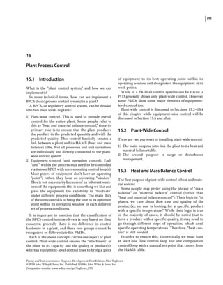
312
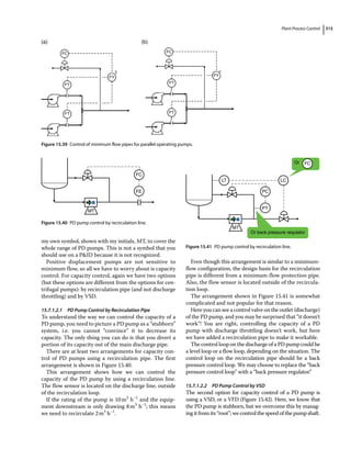
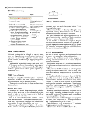
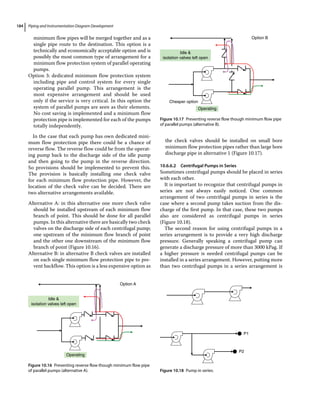
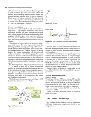
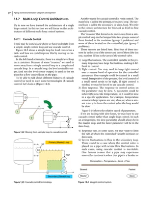
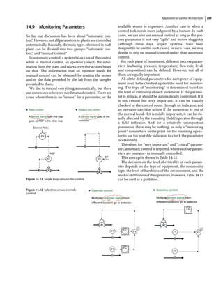
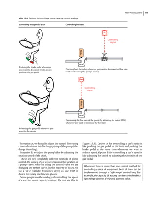
Control Valve Versus VFD
We learned that there are at least two methods of con-
trolling pumps: by control valve and by VFD. Now the
question is, which one should be used? Sometimes when
we are not sure, we use both of them in the form of split‐
range control. If we cannot afford to use both of them (in
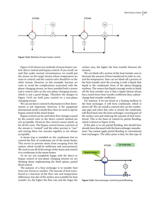
the form of split control), we need to choose one of them.
Traditionally, we use a control valve because it is an older
technology; however, there are cases where a VFD works
better.
The main consciously changing parameter in a water
treatment plant is the flow rate. The flow rate is changing
and we have to find “something” to adjust the flow rate of
different pieces of equipment.
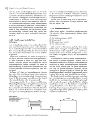
There are mainly two types of device can be used to
adjust the flow rate: control valve and VSD.
A control valve is generally installed on the discharge
line of a pump (or compressor) and the VSD is installed
on the electromotor of the pump (or compressor).
These two methods of adjusting flow rates are named
“final control elements.”
These two methods of controlling the flow rate are
very similar to two methods of controlling the speed of
car we are driving. This analogy can be seen below.
Table 15.9 summarizes some process reasons for using
a control valve or a VFD.
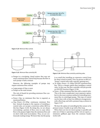
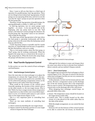
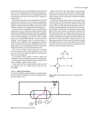
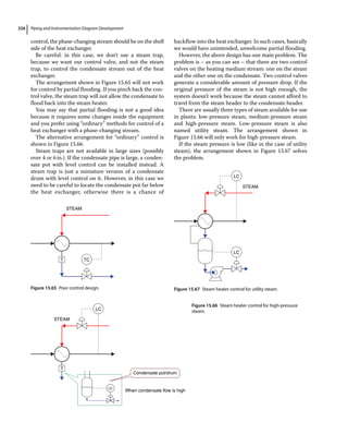
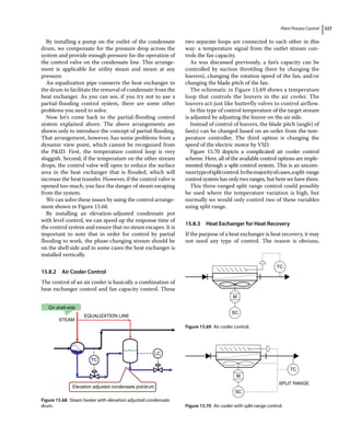
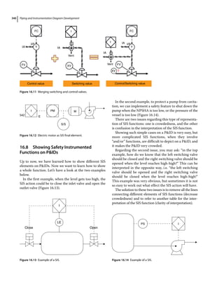
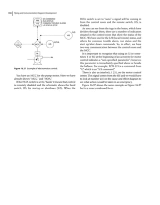
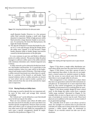
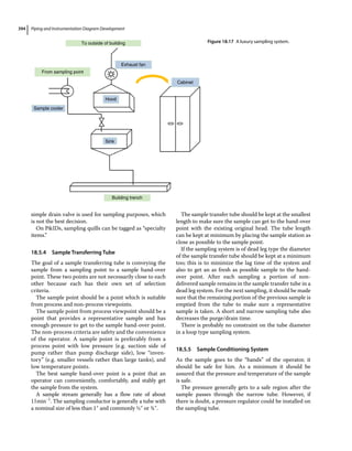
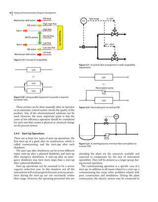
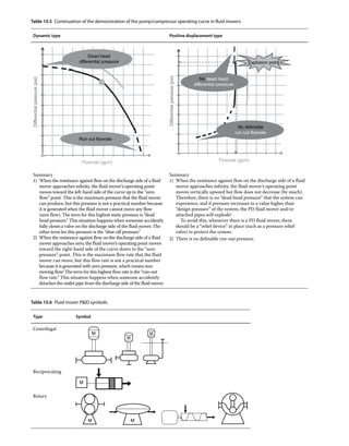
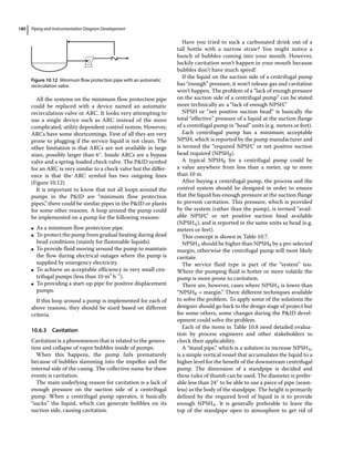
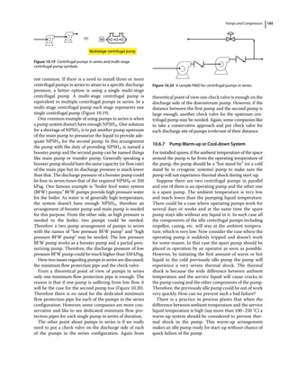
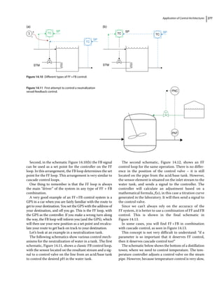
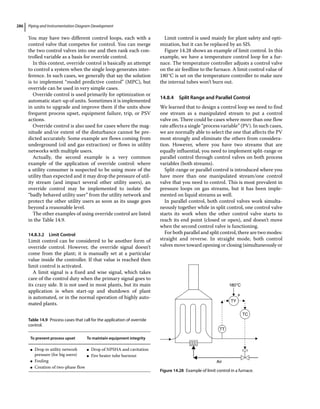
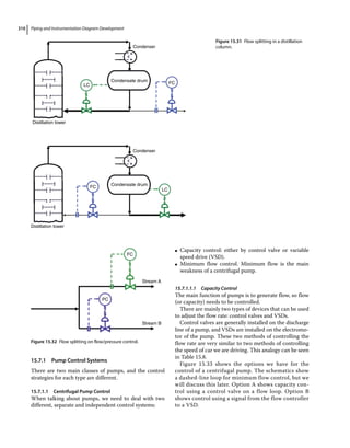
15.7.1.1.2 Minimum Flow Control
The concept of minimum flow control is shown in
Figure 15.34. Let’s assume that this pump has a capacity
of 200m3
h−1
. The vendor specified that the minimum
flow rate of the pump is 100m3
h−1
. We can provide a
recirculation line from the outlet of the pump back into
the inlet line.
If the flow rate into the pump is 165m3
h−1
, the pump
is happy, since its flow is higher than the minimum flow.
In this case, the sensor on the pump outlet sends a signal
to the control valve on the recirculation line and it
remains closed. However, if the flow drops below
100m3
h−1
, for example to 80m3
h−1
, the flow sensor on
the outlet will send a signal to the controller to say: “I am
short of my minimum required flow by 20 m3
h−1
and I
am worried about the pump. Please open the valve
enough to recirculate 20 m3
h−1
, so we can fool the pump
into thinking that the flow is 100 m3
h−1
, and make it
happy,” The control valve on the recirculation line will
be partially opened to provide a flow of 20m3
h−1
, which
is sent back to the inlet to satisfy the minimum flow
condition of 100m3
h−1
, and prevent damage to the
pump. This is the concept of minimum flow control.
It is important to recognize that this “trick” only
increases the flow rate inside the recirculation loop to a
number higher than 100m3
h−1
to “fool” the pump. We
are not able to increase the overall flow in the whole
upstream and downstream piping system; the flow in
those pipes is still 80m3
hr−1
.
The point here is that the sensor should be placed as
close as possible to the pump and within the recircula-
tion loop.
Now the question is whether we need a minimum flow
control loop for all centrifugal pumps or not. The answer
is no! We don’t need minimum flow control loop for all
centrifugal pumps.
The following examples of pumps may not need a min-
imum flow control loop [1]:
●
● Small pumps of less than 5hp; they need it, but they
are inexpensive so we don’t bother to put an expensive
minimum flow control loop on them.
FC
Option A
Option B
FC
FC
FC
VSD
Figure 15.33 Options for centrifugal pump capacity control.
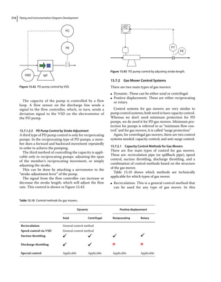
Table 15.9 Options for centrifugal pump capacity control.
Control valve VFD
●
● Generates more shear on the
stream. Not good for shear‐
sensitive liquids like oily
waters, biomaterial, water
carrying flows etc.
●
● Works for all types of piping
circuits
●
● Generates less shear on
the stream
●
● Doesn’t work in systems
where the majority of the
pump head is used to
overcome static pressure
rather than pipe pressure
loss

329. Plant Process Control 313
●
● Pumps in a circulating, closed system: they may not
need a minimum flow control loop because the flow in
such pumps is fairly constant.
However, the following examples of pumps may
require minimum flow control:
●
● Large pumps of 5hp or more
●
● Pumps on the main stream.
The rule of thumb for providing minimum flow con-
trol is as follows:
●
● Power5hp: no minimum flow line is required, as
mentioned before.
●
● 5hpPower10–20hp: continuous minimum flow
line. Instead of going to the expense of installing a
control valve, we can put a restriction orifice (RO) on
this line (Figure 15.35). By doing this, we are always
recirculating a portion of flow, even in cases where
flow to the pump is higher than the minimum flow and
we don’t really need recirculation. Thus, we are con-
tinuously wasting energy. We know that, but the pump
is so small that installing an expensive control loop
for them is hard to justify. (You can picture an RO as a
“frozen” control valve with a specific opening size.)
●
● 10–20hpPower15–30hp: ON/OFF minimum flow
line. This is a cheaper option than installing a control
valve. In this case, the flow controller will just provide
an ON/OFF function (Figure 15.36).
●
● Power35hp: minimum flow line with a control valve.
This is the most complicated, most expensive option,
but it is the most common method of controlling mini-
mum flow in centrifugal pumps. This type of control
can be done with at least two different arrangements:
with a flow loop, and with a pressure loop, as shown in
Figure 15.37.
We have the option of controlling by flow sensor or by
pressure sensor. Usually we go with a flow loop.
When there are two (or more) pumps in parallel and
only one of them is operating and the rest are spares, a
minimum spillback pipe from the common header
works well.
Senses more than 100 m3/hr
so closes the valve
Senses less than 100 m3/hr
so opens the valve
Minimum flow:
100 m3/hr
FV
FV
FC
FC
FIC
FIC
FT
FT
FX
FX
0 m3/hr
80 m3/hr
165 m3/hr
20 m3/hr
165 m3/hr
80 m3/hr
Figure 15.34 Minimum flow control.
RO
Figure 15.35 Minimum flow control by RO.
FC
Figure 15.36 Minimum flow control by switching valve.

330. Piping and Instrumentation Diagram Development
314
The question is what the minimum flow should be
when there are parallel operating pumps. We have three
options for providing minimum flow lines for parallel
operating pumps, as shown in Figure 15.38.
In option 1 one, a shared minimum recirculation pipe
is provided for two operating pumps.
In option 2, dedicate recirculation pipes are provided
at the beginning but they are merged in downstream
before getting to the upstream reservoir.
In option 3, fully dedicated minimum flow pipes are
provided for each pump in parallel arrangement and
both are operating.
The problem with option 1 is that the flow from the two
pumps compensate for each other and the sensor cannot
tell if one pump is starving or not. So the sensor could be
telling you that the system is OK, whereas one of the
pumps could actually be in bad shape. Option 3 may be
the best system, but it is the most expensive option. For
this reason, most companies go with option 2.
In any of the cases at least two different types of ­control
system can be applied on the minimum flow pipe shown
in Figure 15.39.
In schematic (a) the total flow is used for the purpose of
control while in schematic (b) the minimum flow is used.
The issue with schematic (a) is that the control system
cannot “recognize” the pump is suffering from the flow
lower than the minimum flow. The issue with schematic
(b) is that the control system cannot provide the flow to
satisfy both suffering pumps if both pumps are suffering
from flow lower than the minimum flow but with uneven
difference to the minimum flow.
15.7.1.2 Positive Displacement (PD) Pump
Because more than 80% of pumps used in the process
industry are centrifugal pumps, many people are not
familiar with how to control PD pumps. You cannot use
the same arrangement for controlling a PD pump as for a
centrifugal pump; it does not work. If you put a flow loop
on the discharge side of the pump, it won’t change the
flow at all.
There are two main groups of PD pumps: reciprocating
and rotary. Each has its own symbol, but I have invented
FC
Flow control type
FC
Pressure control type
Figure 15.37 Automatic control of
minimum flow.
Option 1:
Option 2:
Option 3:
Figure 15.38 Minimum flow pipes for parallel operating pumps.

331. Plant Process Control 315
my own symbol, shown with my initials, MT, to cover the
whole range of PD pumps. This is not a symbol that you
should use on a PID because it is not recognized.
Positive displacement pumps are not sensitive to
minimum flow, so all we have to worry about is capacity
control. For capacity control, again we have two options
(but these options are different from the options for cen-
trifugal pumps): by recirculation pipe (and not discharge
throttling) and by VSD.
15.7.1.2.1 PD Pump Control by Recirculation Pipe
To understand the way we can control the capacity of a
PD pump, you need to picture a PD pump as a “stubborn”
system, i.e. you cannot “convince” it to decrease its
capacity. The only thing you can do is that you divert a
portion of its capacity out of the main discharge pipe.
There are at least two arrangements for capacity con-
trol of PD pumps using a recirculation pipe. The first
arrangement is shown in Figure 15.40.
This arrangement shows how we can control the
capacity of the PD pump by using a recirculation line.
The flow sensor is located on the discharge line, outside
of the recirculation loop.
If the rating of the pump is 10m3
h−1
and the equip-
ment downstream is only drawing 8m3
h−1
; this means
we need to recirculate 2m3
h−1
.
Even though this arrangement is similar to a minimum‐
flow configuration, the design basis for the recirculation
pipe is different from a minimum‐flow protection pipe.
Also, the flow sensor is located outside of the recircula-
tion loop.
The arrangement shown in Figure 15.41 is somewhat
complicated and not popular for that reason.
Here you can see a control valve on the outlet (discharge)
of the PD pump, and you may be surprised that “it doesn’t
work”! You are right, controlling the capacity of a PD
pump with discharge throttling doesn’t work, but here
we have added a recirculation pipe to make it workable.
The control loop on the discharge of a PD pump could be
a level loop or a flow loop, depending on the situation. The
control loop on the recirculation pipe should be a back
pressure control loop. We may choose to replace the “back
pressure control loop” with a “back pressure regulator.”
15.7.1.2.2 PD Pump Control by VSD
The second option for capacity control of a PD pump is
using a VSD, or a VFD (Figure 15.42). Here, we know that
the PD pump is stubborn, but we overcome this by manag-
ing it from its “root”; we control the speed of the pump shaft.
FC
FT
FY
FT
FC
FT
FY
FT
Σ
(a) (b)
Figure 15.39 Control of minimum flow pipes for parallel operating pumps.
FC
FE
MT
Figure 15.40 PD pump control by recirculation line.
LC
Or
Or back pressure requlator
PC
PT
LT
MT
FC
Figure 15.41 PD pump control by recirculation line.

332. Piping and Instrumentation Diagram Development
316
The capacity of the pump is controlled by a flow
loop. A flow sensor on the discharge line sends a
­
signal to the flow controller, which, in turn, sends a
deviation signal to the VSD on the electromotor of
the PD pump.
15.7.1.2.3 PD Pump Control by Stroke Adjustment
A third type of PD pump control is only for reciprocating
pumps. In the reciprocating type of PD pumps, a mem-
ber does a forward and backward movement repeatedly
in order to achieve the pumping.
The third method of controlling the capacity is appli-
cable only to reciprocating pumps: adjusting the span
of the member’s reciprocating movement, or simply
adjusting the stroke.
This can be done by attaching a servomotor to the
“stroke‐adjustment lever” of the pump.
The signal from the flow controller can increase or
decrease the stroke length, which will adjust the flow
rate. This control is shown in Figure 15.43.
15.7.2 Gas Mover Control Systems
There are two main types of gas movers:
●
● Dynamic. These can be either axial or centrifugal.
●
● Positive displacement. These are either reciprocating
or rotary.
Control systems for gas movers are very similar to
pump control systems; both need to have capacity ­control.
Whereas we don’t need minimum protection for PD
pumps, we do need it for PD gas movers. Minimum pro-
tection for pumps is referred to as “minimum flow con-
trol,” and for gas movers, it is called “surge protection.”
Again, for centrifugal gas movers, there are two control
systems needed: capacity control, and anti‐surge control.
15.7.2.1 Capacity Control Methods for Gas Movers
There are five main types of control for gas movers.
These are: recirculation pipe (or spillback pipe), speed
control, suction throttling, discharge throttling, and a
combination of control methods based on the structure
of the gas mover.
Table 15.10 shows which methods are technically
applicable for which types of gas mover.
●
● Recirculation. This is a general control method that
can be used for any type of gas mover. In this
FC
VSD MT
FE
Figure 15.42 PD pump control by VSD.
FC
FT
FE
Figure 15.43 PD pump control by adjusting stroke length.
Table 15.10 Control methods for gas movers.
Dynamic Positive displacement
Axial Centrifugal Reciprocating Rotary
Recirculation General control method
Speed control via VSD General control method
Suction throttling
Discharge throttling
Special control Applicable Applicable Applicable Applicable

333. Plant Process Control 317
method, a pipe connects the discharge side of gas
mover to its suction side (spillback pipe). A control
loop is placed on the spillback pipe. This arrange-
ment looks very similar to the “minimum flow pro-
tection” system in pipes, but there are plenty of
differences in the details.
●
● Speed control (VSD). Again, you can use this method
of control for all gas movers. In this method, the speed
of the gas mover’s shaft is adjusted through a mecha-
nism. As was mentioned, the “mechanism” could be a
VFD (for electric motors as the drive) or a governor
(for turbines as the drive).
●
● Suction throttling. Suction throttling means putting
the control valve on the suction side of the gas mover.
With a pump, you have the danger of cavitation if you
place the control valve on the suction side, but cavita-
tion is not an issue with gas movers.
●
● Discharge throttling. This means that the control
valve is placed on the discharge side of the gas
mover. This method of control is acceptable to
use with dynamic gas movers, but not with PD
gas movers.
●
● Special control method. Unlike the previous four
control methods, this is not a single control method.
Depending on the type of gas mover, a few extra
­
control methods could be available. We call all of
these “gas mover‐specific” control methods “special
control.” For example, in axial gas movers such as
blowers and air coolers, we can adjust the flow rate by
changing the pitch or angle of the blades.
In the above paragraph, I explained the different types
of control that are “technically” possible; however, not all
of them are economically acceptable in each application.
Table 15.11 gives the applicability of each of the control
methods mentioned.
The items in Table 15.11 are expanded below:
●
● Recirculation. This method is not very economical
because when you recirculate back to the suction side,
you are expanding the gas and therefore wasting
energy (Figure 15.44).
Here we have a recirculation line with a check valve.
We have included a cooler on the line because with
compression, you get an increase in temperature and
you may need to cool the recirculated gas before it goes
back into the suction side of the gas mover. We also
have a control valve on this line to prevent all of the
flow from going through this attractive route of less
resistance.
Table 15.11 Control methods for gas movers.
Dynamic Positive displacement
Axial Centrifugal Reciprocating Rotary
Recirculation Not economical, especially for high‐pressure applications
Speed control via
VSD
General control method
Suction throttling Common Common Not good practice Not good practice
Discharge throttling Not economical Not economical
Special control ●
● Blade pitch adjustment:
most common
●
● Guide vane
adjustment
●
● Suction valve unloading:
most common
●
● Clearance pocket adjustment
●
● Slide valve
adjustment
FT
FC
M M
PC
PT
Figure 15.44 Recirculation control for a gas mover.

334. Piping and Instrumentation Diagram Development
318
There are two options for a control loop here: flow
loop or pressure loop, and as flow and pressure are
interrelated, both of them are theoretically acceptable.
The decision of whether to use a flow control loop or a
pressure control loop could be based on some other
parameters. For example, pressure sensors generally
have higher rangeability and if your flow surges a lot a
pressure loop may be a better option.
The other case is when you are dealing with very high
discharge pressures. In such cases, high design pressure
flow meters could be overly expensive and not justifiable.
This may direct you to use a pressure control loop instead
of a flow control loop.
●
● Speed control (VSD). This method can be used with all
gas movers.
Figure 15.45 shows the control of a gas mover by VSD
when its drive is an electric motor.
Some companies use the symbol “SC” in their sche-
matics, meaning “speed control.”
Some other companies use the acronym “VFD.”
Figure 15.46 shows the same VSD control on a steam
turbine‐driven gas mover. Here the device that works to
change the speed of turbine shaft is a “governor.”
●
● Suction throttling. Suction throttling can be used for
all types of gas movers but is really only popular with
centrifugal gas movers (Figure 15.47).
●
● Discharge throttling. Although this method can be used
for all dynamic type gas movers, it is not economical. By
adjusting the valve on the discharge side of a gas mover,
we are partially expanding a gas that we had already com-
pressed (and spent money to do so) through the gas
mover (Figure 15.48). This is a waste of energy. However,
this is not much of a factor when dealing with gas movers
with small compression ratios, such as fans and blowers.
FC
SC
SC
PT
PT
FT
M
M
Figure 15.45 Speed control of a motor‐driven gas
mover.
T
FT
FC
Gov
Figure 15.46 Speed control of a turbine‐driven gas mover.
M
FT
FC
PT
PC
M
Figure 15.47 Suction‐throttling control of a gas
mover.
M
FT
FC
PT
PC
M
Figure 15.48 Discharge‐throttling control of a
gas mover.

335. Plant Process Control 319
●
● Special control method. This is a combination of
capacity control methods for gas movers that uses
some adjustable element in the structure of the gas
mover to control its capacity. To be able to explain all
of these methods, one needs to know the detailed
structure of gas movers, which is beyond the scope of
this book. So here, we instead explain only two simple
“special control methods.”
Figure 15.49 shows “blade pitch control,” which is a
special control method used only for axial gas movers.
One famous application of an “axial gas mover” is in air
coolers.
In the air cooler shown below, the outlet temperature
of the hot stream is adjusted by the air flow rate. The air
flow rate is adjusted by the angle (pitch) of the propeller
blades.
In the second example, in Figure 15.50, another spe-
cial control method is shown that is applicable only to
centrifugal gas movers. In centrifugal gas movers, there
is an element installed in the inlet of the gas mover,
called a “guide vane.” By controlling the position of the
guide vane, the capacity of the gas mover can be adjusted.
To have a better picture of this, you can visualize the
guide vane as being similar to a built‐in control valve on
the suction side of the gas mover.
15.7.3 Anti‐Surge Control
When we talk about surge control, we have the same prob-
lem