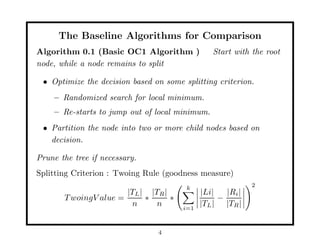
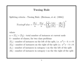
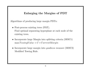
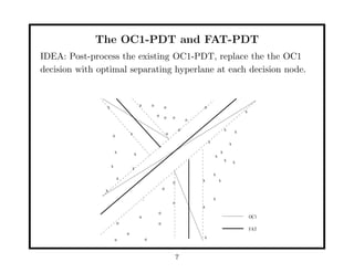
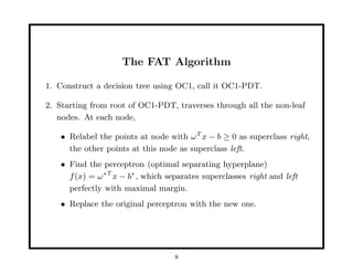
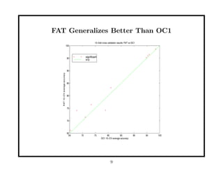
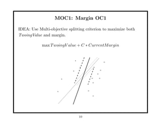
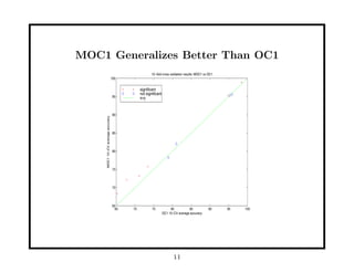
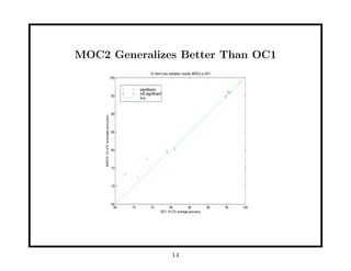
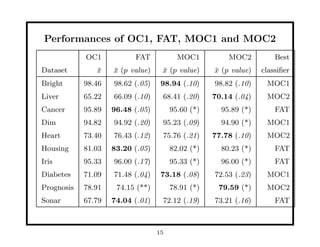
This document discusses methods for improving perceptron decision trees (PDTs) by enlarging their margins. It proposes three algorithms: 1. FAT (Find-And-Replace Trees) post-processes existing decision trees by replacing each node's decision with an optimal separating hyperplane found via perceptron learning, maximizing the margin. 2. MOC1 (Margin OC1) modifies the OC1 algorithm to use a multi-objective splitting criterion that maximizes both information gain and margin size. 3. MOC2 modifies the splitting criterion (Twoing rule) to incorporate margin. Experimental results show FAT and MOC1 generalize better than the basic OC1 algorithm on benchmark datasets.

1. Enlarging the Margins in Perceptron
Decision Trees
Kristin P. Bennett, Donghui Wu
Department of Mathematical Sciences
Rensselaer Polytechnic Institute
bennek@rpi.edu, wud2@rpi.edu
Nello Cristianini John Shawe-Taylor
Dept of Engineering Mathematics Dept of Computer Science
University of Bristol Royal Holloway, University of London
nello.cristianini@bristol.ac.uk jst@dcs.rhbnc.ac.uk
0-0

2. Perceptron Decision Trees
Definition 0.1 Perceptron Decision Trees (PDT), are decision
trees in which each internal node is associated with a hyperplane in
general position in the input space, i.e. the decision is constructed
using a linear combination of attributes, instead of one attribute.
w1 x x x x
x x x
x x w3
w1 x
o
x o o o
o o o o
x o
w2 w3 x o o
x o
x o
o o o
x x
x o o x x
w2
1

3. Which Decision Is Better?
– Capacity Control of Linear Classifier
Construct a linear classifier: f (x) = wT x − b, i.e.
find a vector w ∈ Rn and a scalar b such that
f (xi ) = wT xi − b ≥1 if yi = 1,
f (xi ) = wT xi − b ≤ −1 if yi = −1,
i = 1, . . . ,
2

4. Large Margin PDTs Generalize Better
Theorem 0.1 Suppose we are able to classify an m sample of
labeled examples using a perception decision tree and suppose that
the tree obtained contained K decision nodes with margins γi at
node i, then we can bound the generalization error with probability
greater than 1 − δ to be less than
130R2 (4m)K+1 2K
K
D log(4em) log(4m) + log
m (K + 1)δ
K 1
where D = i=1 γi .
2
3

5. The Baseline Algorithms for Comparison
Algorithm 0.1 (Basic OC1 Algorithm ) Start with the root
node, while a node remains to split
• Optimize the decision based on some splitting criterion.
– Randomized search for local minimum.
– Re-starts to jump out of local minimum.
• Partition the node into two or more child nodes based on
decision.
Prune the tree if necessary.
Splitting Criterion : Twoing Rule (goodness measure)
k 2
|TL | |TR | |Li| |Ri |
T woingV alue = ∗ ∗ −
n n i=1
|TL | |TR |
4

6. Twoing Rule
Splitting criteria - Twoing Rule: (Breiman, et al. (1984))
k 2
|TL | |TR | |Li| |Ri |
T woingV alue = ∗ ∗ −
n n i=1
|TL | |TR |
where
n = |TL | + |TR | - total number of instances at current node
k - number of classes, for two class problems
|TL | - number of instances on the left of the split, i.e. wT x − b >= 0
|TR | - number of instances on the right of the split i.e. wT x − b < 0
|Li | - number of instances in category i on the the left of the split
|Ri | - number of instances in category i on the the right of the split
5

7. Enlarging the Margins of PDT
Algorithms of producing large margin PDTs:
• Post-process existing trees (FAT).
Find optimal separating hyperplane at each node of the
existing trees.
• Incorporate large Margin into splitting criteria (MOC1)
max T woingV alue + C ∗ CurrentM argin
• Incorporate large margin into goodness measure (MOC2)
Modified Towing Rule.
6

8. The OC1-PDT and FAT-PDT
IDEA: Post-process the existing OC1-PDT, replace the the OC1
decision with optimal separating hyperlane at each decision node.
x o o o o
x
o o o o
o x x
x x o
x x
x x x
x
x x
x x
x
x x x
o
x o
; x
o
x
o
o OC1
o o
FAT
o
o x
o
7

9. The FAT Algorithm
1. Construct a decision tree using OC1, call it OC1-PDT.
2. Starting from root of OC1-PDT, traverses through all the non-leaf
nodes. At each node,
• Relabel the points at node with ω T x − b ≥ 0 as superclass right,
the other points at this node as superclass left.
• Find the perceptron (optimal separating hyperplane)
f (x) = ω ∗ T x − b∗ , which separates superclasses right and left
perfectly with maximal margin.
• Replace the original perceptron with the new one.
8

10. FAT Generalizes Better Than OC1
10−fold cross validation results: FAT vs OC1
100
95 significant
x=y
90
FAT 10−CV average accuracy
85
80
75
70
65
65 70 75 80 85 90 95 100
OC1 10−CV average accuracy
9

11. MOC1: Margin OC1
IDEA: Use Multi-objective splitting criterion to maximize both
TwoingValue and margin.
max T woingV alue + C ∗ CurrentM argin
x
o
x o
x o
o
x o o
x o
x o
o
10

12. MOC1 Generalizes Better Than OC1
10−fold cross validation results: MOC1 vs OC1
100
significant
not significant
95 x=y
90
MOC1 10−CV average accuracy
85
80
75
70
65
65 70 75 80 85 90 95 100
OC1 10−CV average accuracy
11

13. The MOC2 Algorithm
IDEA: Modify Twoing Criterion to allow “soft-margin”.
Want both high accuracy and strong separation/margin.
k k
|M TL | |M TR | |Li | |Ri | |M Li | |M Ri |
T woingV alue = ∗ ∗ − ∗ −
n n |TL | |TR | |M TL | |M TR |
i=1 i=1
x x o
x x o
x o
x
o o
x
x x x x o
x o o
o o
x x o o o
x o o
x x o o
x x
o
o
x o
x o
x
wx=b+1 wx = b wx=b-1
12

14. The Modified Twoing Rule
k k
|M TL | |M TR | |Li | |Ri | |M Li | |M Ri |
T woingV alue = ∗ ∗ − ∗ −
n n |TL | |TR | |M TL | |M TR |
i=1 i=1
where n = |TL | + |TR | - total number of instances at current node
k - number of classes, for two class problems
|TL | - number of instances on the left of the split, i.e. wT x − b >= 0
|TR | - number of instances on the right of the split i.e. wT x − b < 0
|Li | - number of instances in category i on the the left of the split
|Ri | - number of instances in category i on the the right of the split
|M TL | - number of instances on the left of the split, wT x − b >= 1
|M TR | - number of instances on the right of the split wT x − b <= −1
|M Li | - number of instances in category i with wT x − b >= 1
|M Ri | - number of instances in category i with wT x − b <= −1
13

15. MOC2 Generalizes Better Than OC1
10−fold cross validation results: MOC2 vs OC1
100
significant
95
not significant
x=y
90
MOC2 10−CV average accuracy
85
80
75
70
65
65 70 75 80 85 90 95 100
OC1 10−CV average accuracy
14

16. Performances of OC1, FAT, MOC1 and MOC2
OC1 FAT MOC1 MOC2 Best
Dataset x
¯ x (p value)
¯ x (p value)
¯ x (p value)
¯ classifier
Bright 98.46 98.62 (.05) 98.94 (.10) 98.82 (.10) MOC1
Liver 65.22 66.09 (.10) 68.41 (.20) 70.14 (.04) MOC2
Cancer 95.89 96.48 (.05) 95.60 (*) 95.89 (*) FAT
Dim 94.82 94.92 (.20) 95.23 (.09) 94.90 (*) MOC1
Heart 73.40 76.43 (.12) 75.76 (.21) 77.78 (.10) MOC2
Housing 81.03 83.20 (.05) 82.02 (*) 80.23 (*) FAT
Iris 95.33 96.00 (.17) 95.33 (*) 96.00 (*) FAT
Diabetes 71.09 71.48 (.04) 73.18 (.08) 72.53 (.23) MOC1
Prognosis 78.91 74.15 (**) 78.91 (*) 79.59 (*) MOC2
Sonar 67.79 74.04 (.01) 72.12 (.19) 73.21 (.16) FAT
15

17. Conclusions
• Generalization error of PDT is bounded by function of
margins, tree size, and training set size.
• Three algorithms to control capacity of PDT investigated:
– Post-processing existing trees (FAT)
– Incorporating margins into splitting criteria:
∗ Multicriteria splitting rule (MOC1)
∗ Soft-margin modified twoing-rule (MOC2).
• Theoretically and empirically enlarged margin PDT performed
better.
16