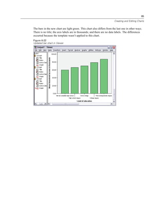
Downloaded 81 times
![4
Chapter 1
An icon next to each variable provides information about data type and level of measurement.
Measurement Data Type
Level Numeric String Date Time
Scale (Continuous) n/a
Ordinal
Nominal
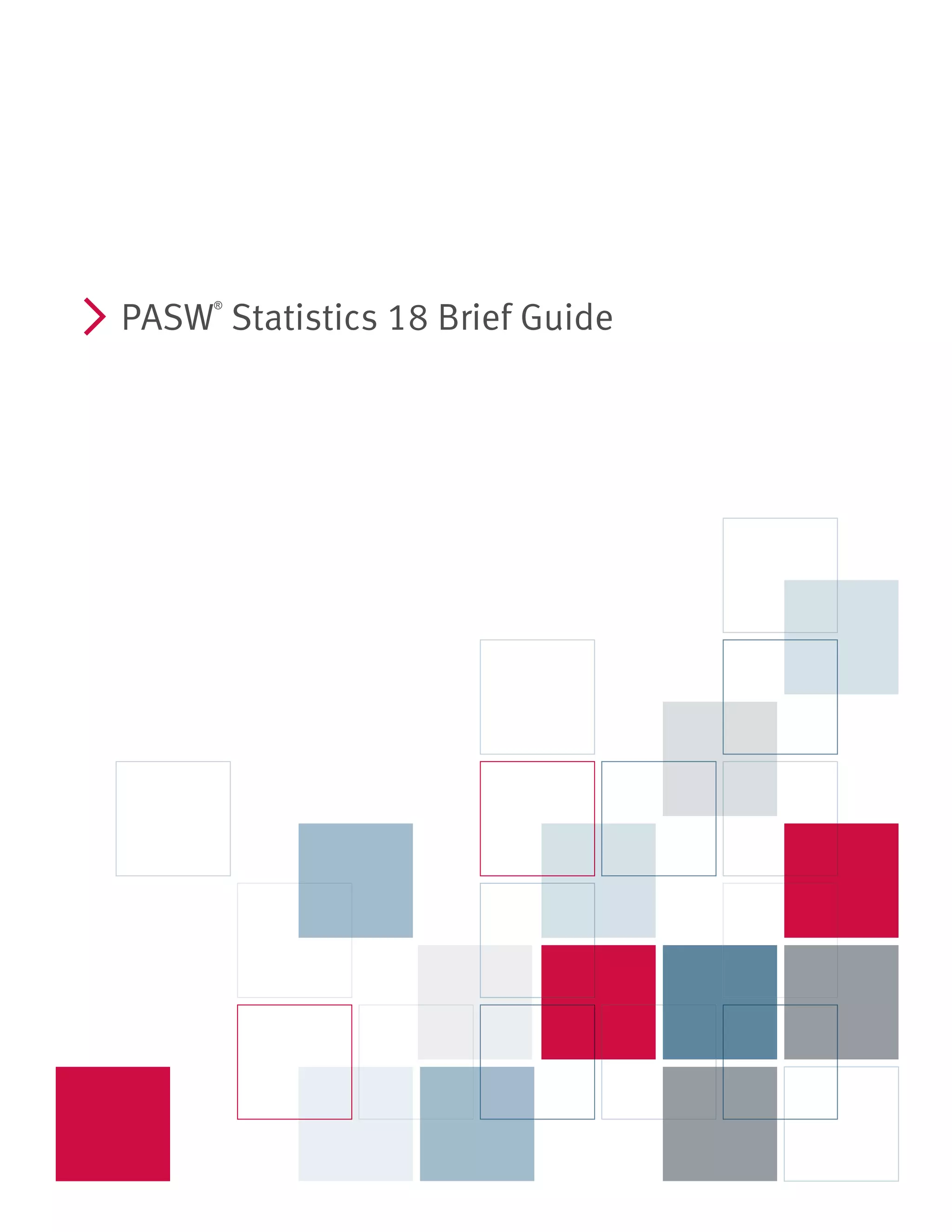
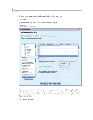
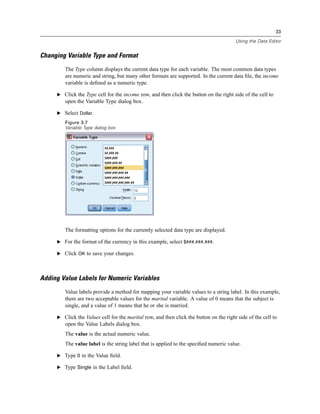
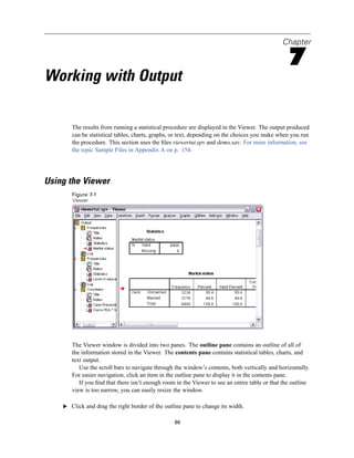
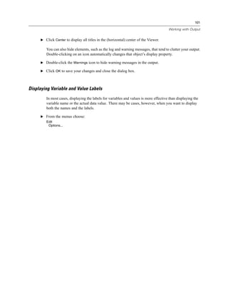
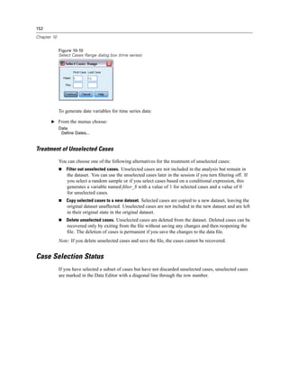
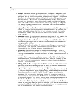
E Click the variable Income category in thousands [inccat].
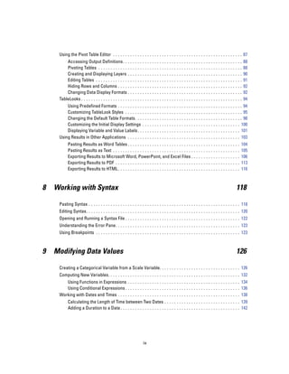
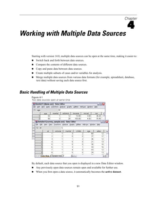
Figure 1-6
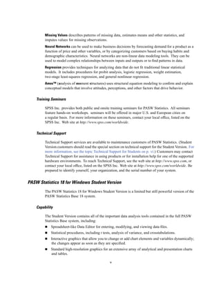
Variable labels and names in the Frequencies dialog box
If the variable label and/or name appears truncated in the list, the complete label/name is displayed
when the cursor is positioned over it. The variable name inccat is displayed in square brackets
after the descriptive variable label. Income category in thousands is the variable label. If there
were no variable label, only the variable name would appear in the list box.
You can resize dialog boxes just like windows, by clicking and dragging the outside borders or
corners. For example, if you make the dialog box wider, the variable lists will also be wider.](https://image.slidesharecdn.com/paswstatistics18briefguide-121129031530-phpapp02/85/Pasw-statistics-18-brief-guide-14-320.jpg)
![5
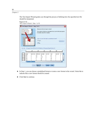
Introduction
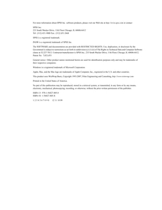
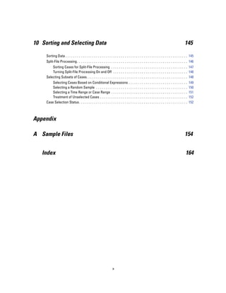
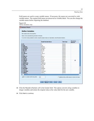
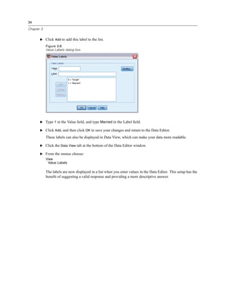
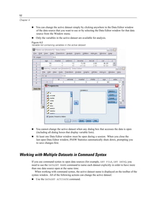
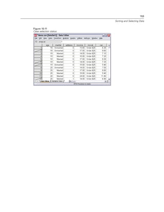
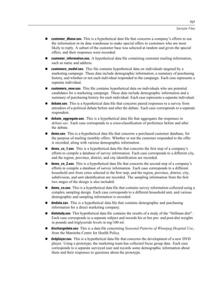
Figure 1-7
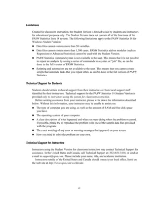
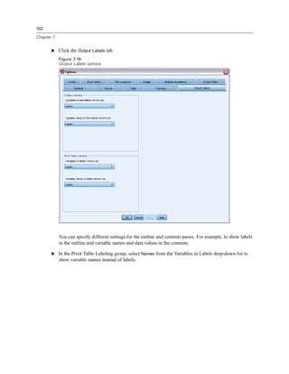
Resized dialog box
In the dialog box, you choose the variables that you want to analyze from the source list on the
left and drag and drop them into the Variable(s) list on the right. The OK button, which runs the
analysis, is disabled until at least one variable is placed in the Variable(s) list.
In many dialogs, you can obtain additional information by right-clicking any variable name
in the list.
E Right-click Income category in thousands [inccat] and choose Variable Information.
E Click the down arrow on the Value labels drop-down list.
Figure 1-8
Defined labels for income variable
All of the defined value labels for the variable are displayed.](https://image.slidesharecdn.com/paswstatistics18briefguide-121129031530-phpapp02/85/Pasw-statistics-18-brief-guide-15-320.jpg)
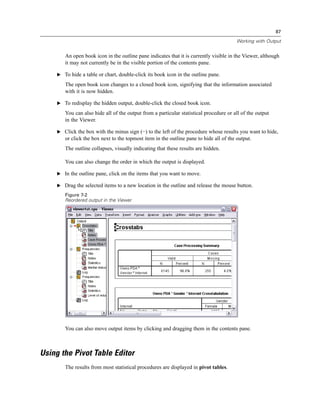
![6
Chapter 1
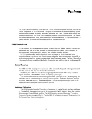
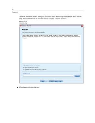
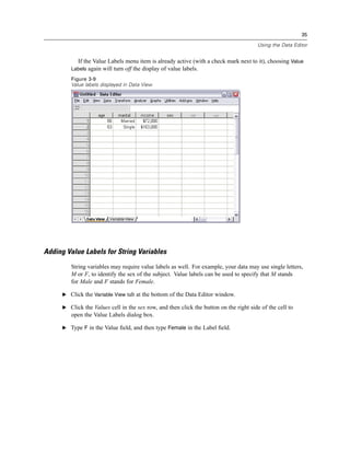
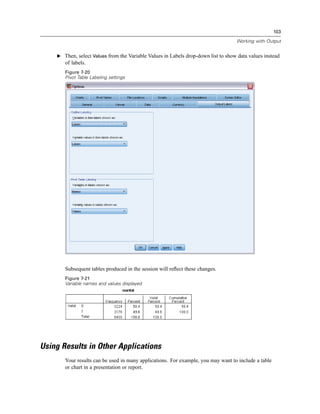
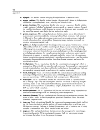
E Click Gender [gender] in the source variable list and drag the variable into the target Variable(s)
list.
E Click Income category in thousands [inccat] in the source list and drag it to the target list.
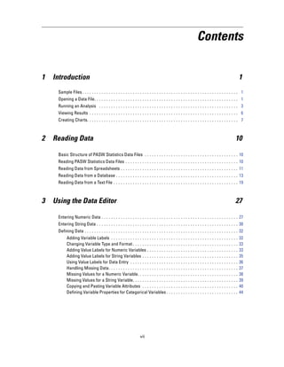
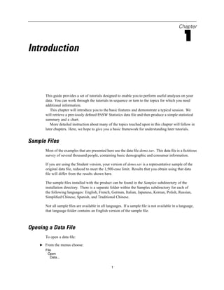
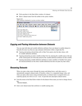
Figure 1-9
Variables selected for analysis
E Click OK to run the procedure.
Viewing Results
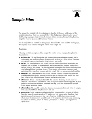
Figure 1-10
Viewer window
Results are displayed in the Viewer window.
You can quickly go to any item in the Viewer by selecting it in the outline pane.](https://image.slidesharecdn.com/paswstatistics18briefguide-121129031530-phpapp02/85/Pasw-statistics-18-brief-guide-16-320.jpg)
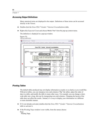
![7
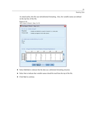
Introduction
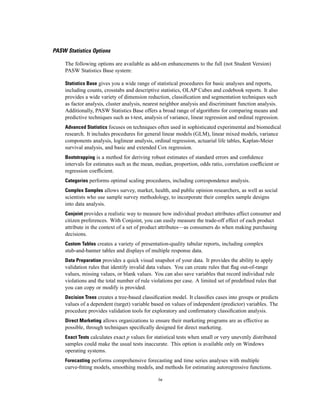
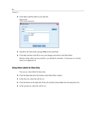
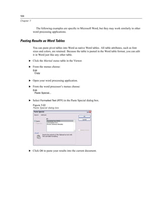
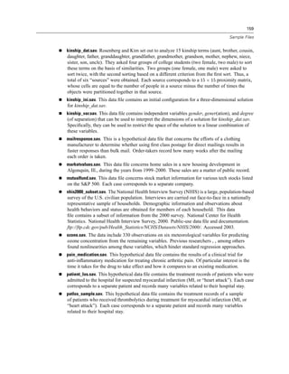
E Click Income category in thousands [inccat].
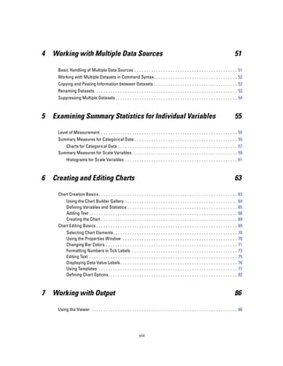
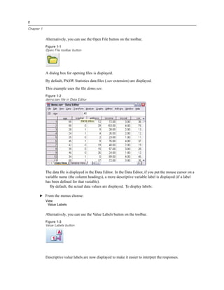
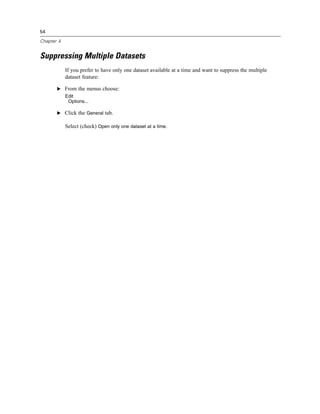
Figure 1-11
Frequency table of income categories
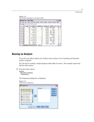
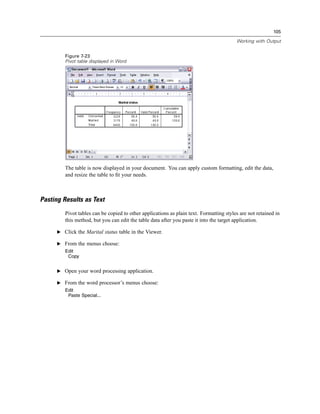
The frequency table for income categories is displayed. This frequency table shows the number
and percentage of people in each income category.
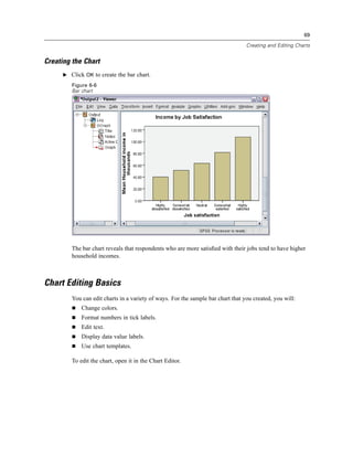
Creating Charts
Although some statistical procedures can create charts, you can also use the Graphs menu to
create charts.
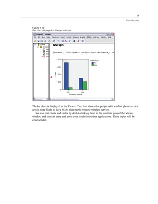
For example, you can create a chart that shows the relationship between wireless telephone
service and PDA (personal digital assistant) ownership.
E From the menus choose:
Graphs
Chart Builder...
E Click the Gallery tab (if it is not selected).
E Click Bar (if it is not selected).
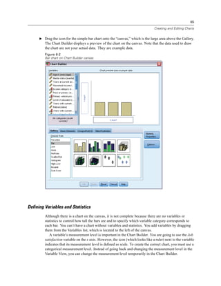
E Drag the Clustered Bar icon onto the canvas, which is the large area above the Gallery.](https://image.slidesharecdn.com/paswstatistics18briefguide-121129031530-phpapp02/85/Pasw-statistics-18-brief-guide-17-320.jpg)
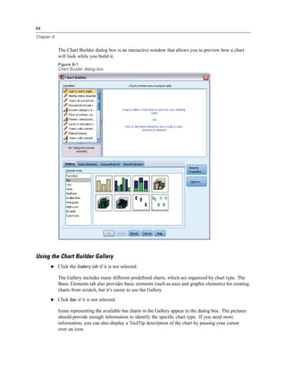
![8
Chapter 1
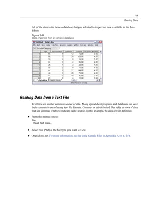
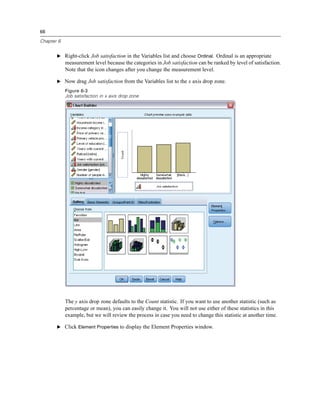
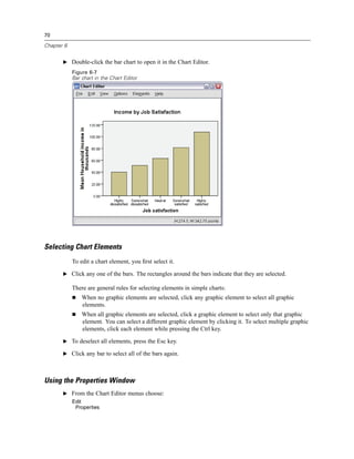
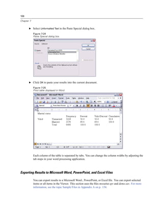
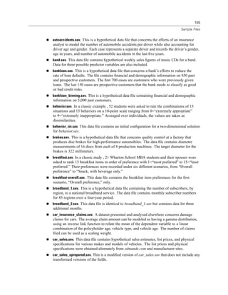
Figure 1-12
Chart Builder dialog box
E Scroll down the Variables list, right-click Wireless service [wireless], and then choose Nominal
as its measurement level.
E Drag the Wireless service [wireless] variable to the x axis.
E Right-click Owns PDA [ownpda] and choose Nominal as its measurement level.
E Drag the Owns PDA [ownpda] variable to the cluster drop zone in the upper right corner of
the canvas.
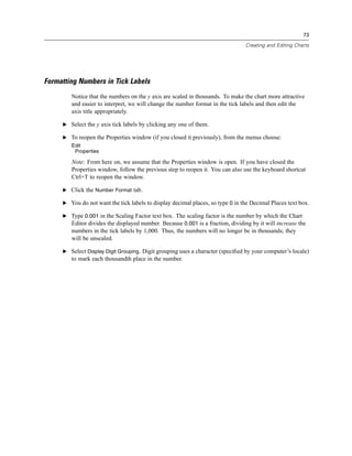
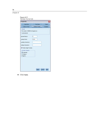
E Click OK to create the chart.](https://image.slidesharecdn.com/paswstatistics18briefguide-121129031530-phpapp02/85/Pasw-statistics-18-brief-guide-18-320.jpg)

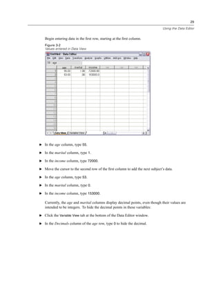
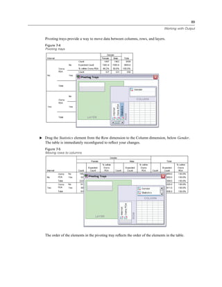
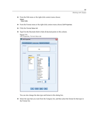
![45
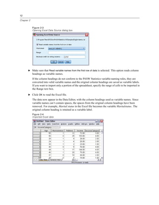
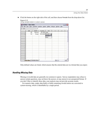
Using the Data Editor
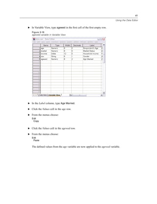
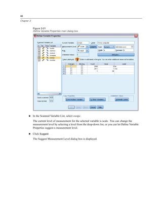
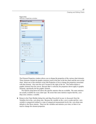
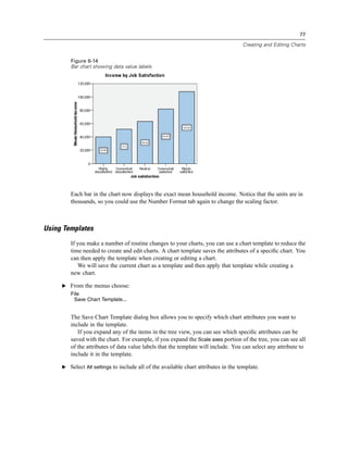
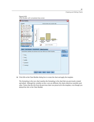
Figure 3-20
Initial Define Variable Properties dialog box
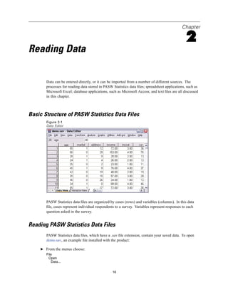
In the initial Define Variable Properties dialog box, you select the nominal or ordinal variables for
which you want to define value labels and/or other properties.
E Drag and drop Owns computer [ownpc] through Owns VCR [ownvcr] into the Variables to
Scan list.
You might notice that the measurement level icons for all of the selected variables indicate that
they are scale variables, not categorical variables. All of the selected variables in this example
are really categorical variables that use the numeric values 0 and 1 to stand for No and Yes,
respectively—and one of the variable properties that we’ll change with Define Variable Properties
is the measurement level.
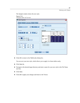
E Click Continue.](https://image.slidesharecdn.com/paswstatistics18briefguide-121129031530-phpapp02/85/Pasw-statistics-18-brief-guide-55-320.jpg)

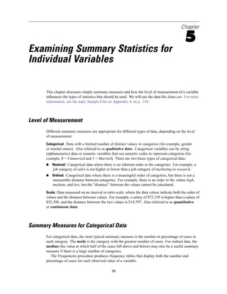
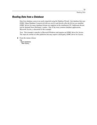
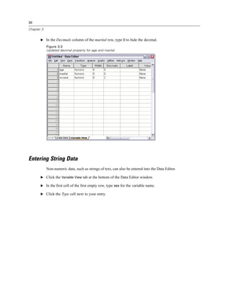
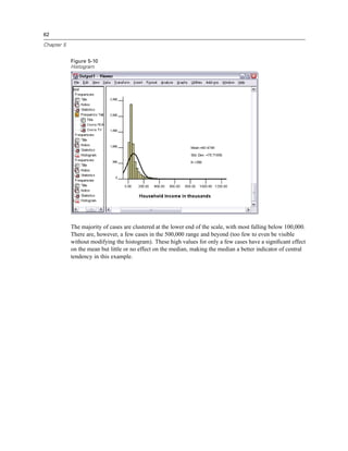
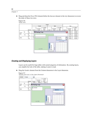
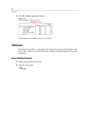
![56
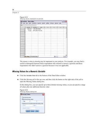
Chapter 5
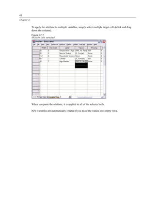
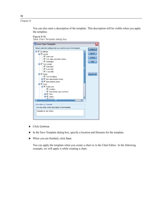
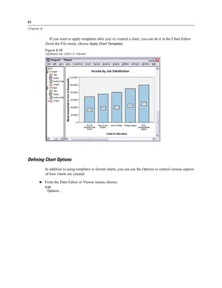
E From the menus choose:
Analyze
Descriptive Statistics
Frequencies...
Note: This feature requires the Statistics Base option.
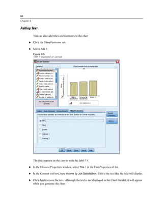
E Select Owns PDA [ownpda] and Owns TV [owntv] and move them into the Variable(s) list.
Figure 5-1
Categorical variables selected for analysis
E Click OK to run the procedure.](https://image.slidesharecdn.com/paswstatistics18briefguide-121129031530-phpapp02/85/Pasw-statistics-18-brief-guide-66-320.jpg)
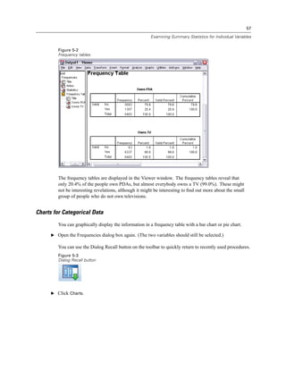
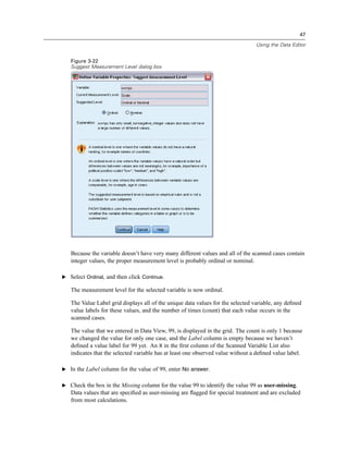
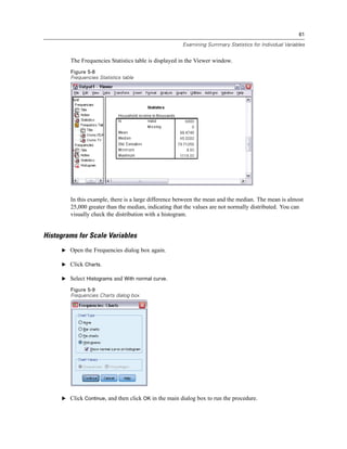
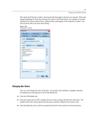
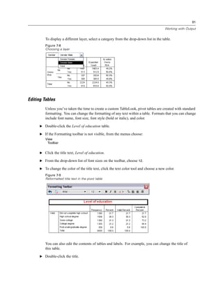
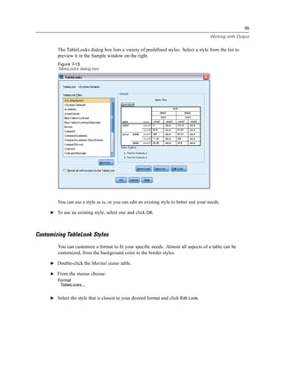
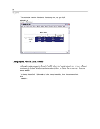
![59
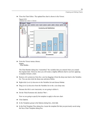
Examining Summary Statistics for Individual Variables
Summary Measures for Scale Variables
There are many summary measures available for scale variables, including:
Measures of central tendency. The most common measures of central tendency are the mean
(arithmetic average) and median (value at which half the cases fall above and below).
Measures of dispersion. Statistics that measure the amount of variation or spread in the data
include the standard deviation, minimum, and maximum.
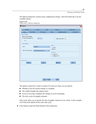
E Open the Frequencies dialog box again.
E Click Reset to clear any previous settings.
E Select Household income in thousands [income] and move it into the Variable(s) list.
Figure 5-6
Scale variable selected for analysis
E Click Statistics.](https://image.slidesharecdn.com/paswstatistics18briefguide-121129031530-phpapp02/85/Pasw-statistics-18-brief-guide-69-320.jpg)
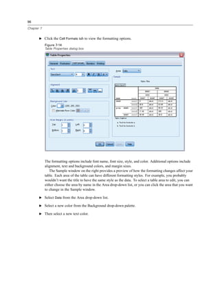
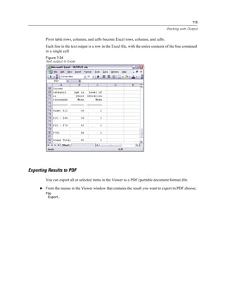
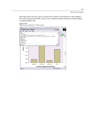

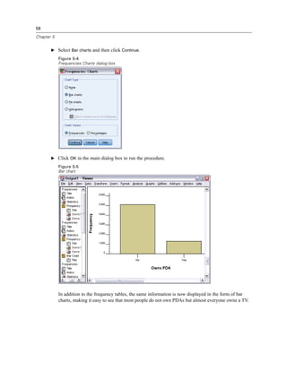
![119
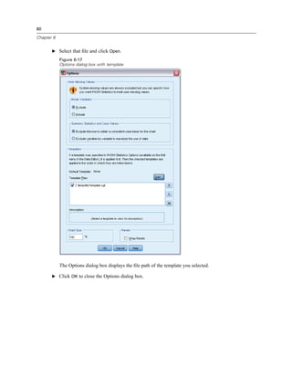
Working with Syntax
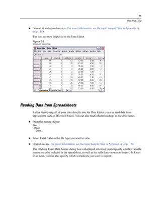
The Frequencies dialog box opens.
Figure 8-1
Frequencies dialog box
E Select Marital status [marital] and move it into the Variable(s) list.
E Click Charts.
E In the Charts dialog box, select Bar charts.
E In the Chart Values group, select Percentages.
E Click Continue.
E Click Paste to copy the syntax created as a result of the dialog box selections to the Syntax Editor.
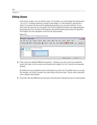
Figure 8-2
Frequencies syntax
E To run the syntax currently displayed, from the menus choose:
Run
Selection](https://image.slidesharecdn.com/paswstatistics18briefguide-121129031530-phpapp02/85/Pasw-statistics-18-brief-guide-129-320.jpg)
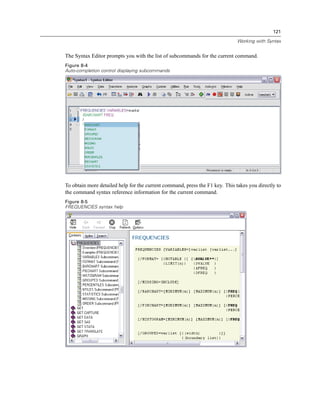
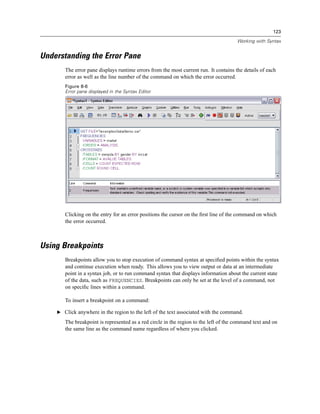

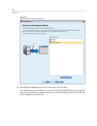
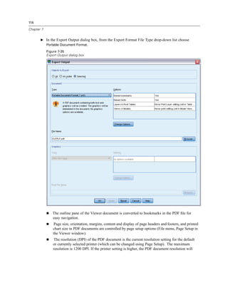
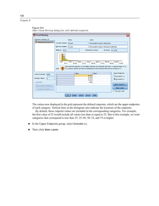
![127
Modifying Data Values
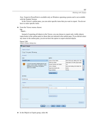
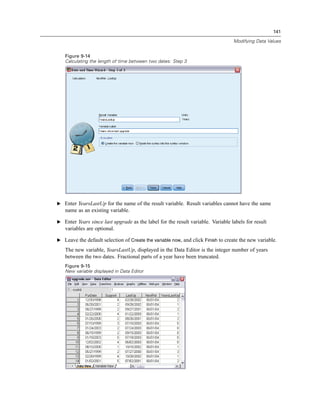
Figure 9-1
Initial Visual Binning dialog box
In the initial Visual Binning dialog box, you select the scale and/or ordinal variables for which you
want to create new, binned variables. Binning means taking two or more contiguous values and
grouping them into the same category.
Since Visual Binning relies on actual values in the data file to help you make good binning
choices, it needs to read the data file first. Since this can take some time if your data file contains
a large number of cases, this initial dialog box also allows you to limit the number of cases to
read (“scan”). This is not necessary for our sample data file. Even though it contains more than
6,000 cases, it does not take long to scan that number of cases.
E Drag and drop Household income in thousands [income] from the Variables list into the Variables
to Bin list, and then click Continue.](https://image.slidesharecdn.com/paswstatistics18briefguide-121129031530-phpapp02/85/Pasw-statistics-18-brief-guide-137-320.jpg)
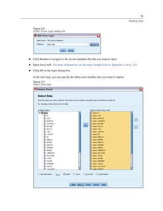
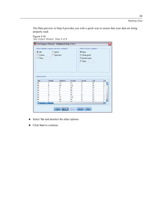
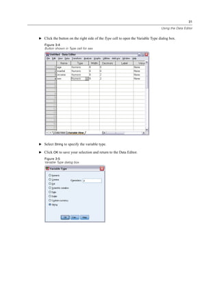
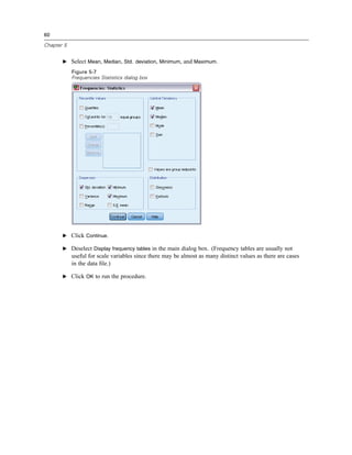
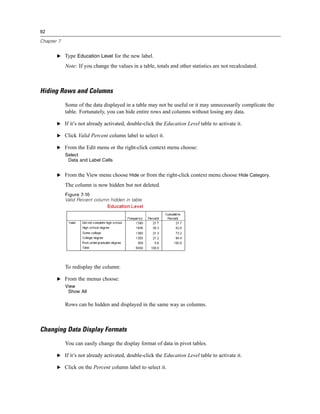
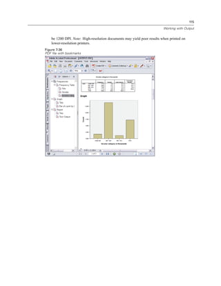
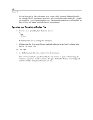
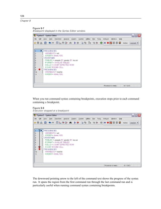
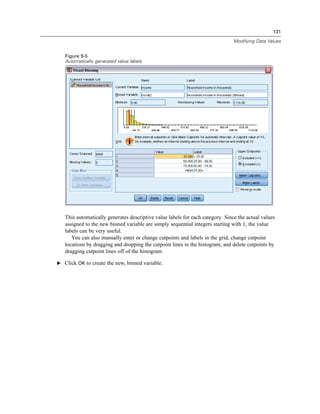
![128
Chapter 9
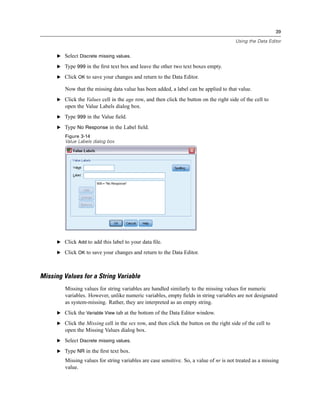
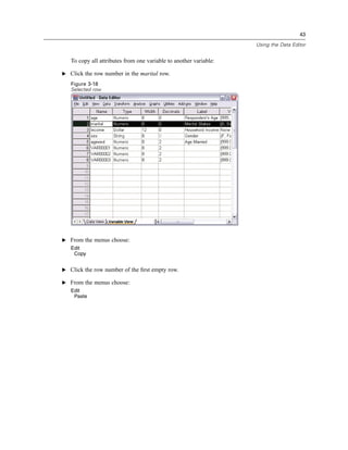
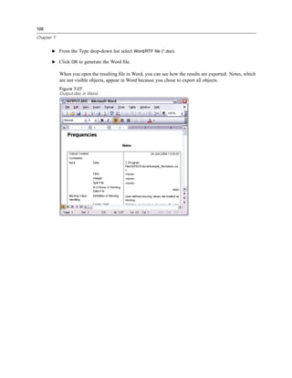
Figure 9-2
Main Visual Binning dialog box
E In the main Visual Binning dialog box, select Household income in thousands [income] in the
Scanned Variable List.
A histogram displays the distribution of the selected variable (which in this case is highly skewed).
E Enter inccat2 for the new binned variable name and Income category [in thousands] for the
variable label.
E Click Make Cutpoints.](https://image.slidesharecdn.com/paswstatistics18briefguide-121129031530-phpapp02/85/Pasw-statistics-18-brief-guide-138-320.jpg)
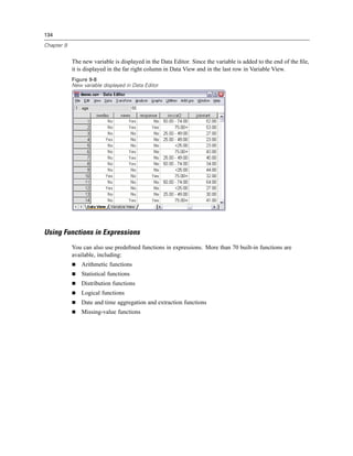
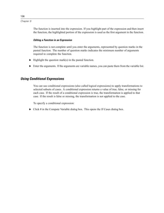
![132
Chapter 9
The new variable is displayed in the Data Editor. Since the variable is added to the end of the file,
it is displayed in the far right column in Data View and in the last row in Variable View.
Figure 9-6
New variable displayed in Data Editor
Computing New Variables
Using a wide variety of mathematical functions, you can compute new variables based on highly
complex equations. In this example, however, we will simply compute a new variable that is the
difference between the values of two existing variables.
The data file demo.sav contains a variable for the respondent’s current age and a variable for the
number of years at current job. It does not, however, contain a variable for the respondent’s age at
the time he or she started that job. We can create a new variable that is the computed difference
between current age and number of years at current job, which should be the approximate age at
which the respondent started that job.
E From the menus in the Data Editor window choose:
Transform
Compute Variable...
E For Target Variable, enter jobstart.
E Select Age in years [age] in the source variable list and click the arrow button to copy it to the
Numeric Expression text box.
E Click the minus (–) button on the calculator pad in the dialog box (or press the minus key on
the keyboard).](https://image.slidesharecdn.com/paswstatistics18briefguide-121129031530-phpapp02/85/Pasw-statistics-18-brief-guide-142-320.jpg)
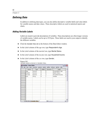
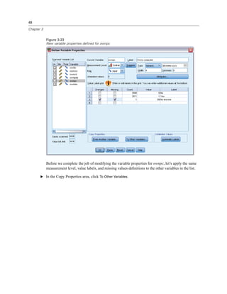
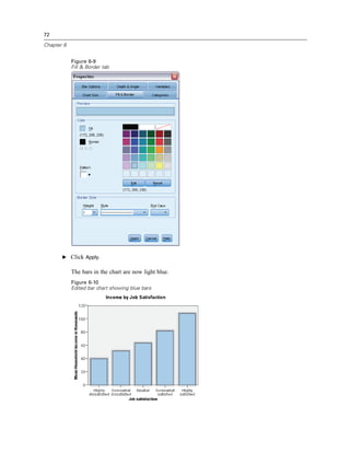
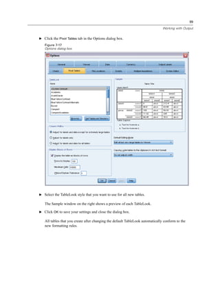
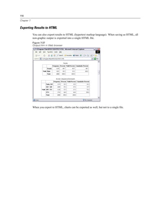
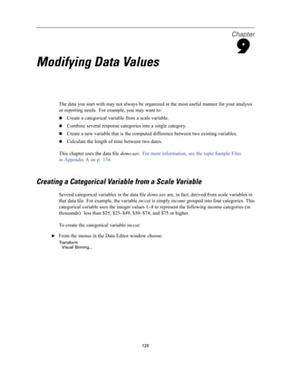
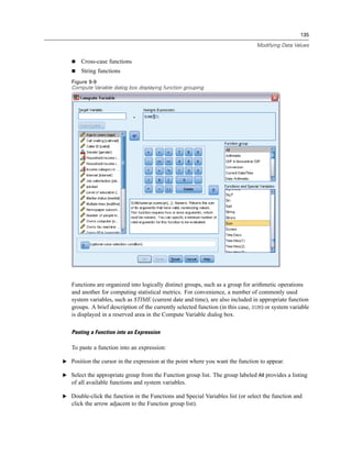
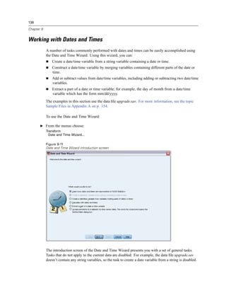
![133
Modifying Data Values
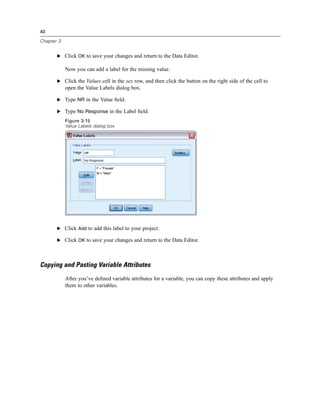
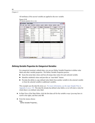
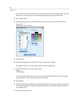
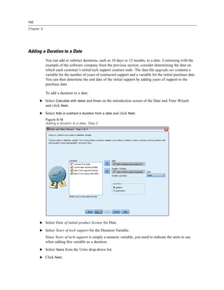
E Select Years with current employer [employ] and click the arrow button to copy it to the expression.
Figure 9-7
Compute Variable dialog box
Note: Be careful to select the correct employment variable. There is also a recoded categorical
version of the variable, which is not what you want. The numeric expression should be
age–employ, not age–empcat.
E Click OK to compute the new variable.](https://image.slidesharecdn.com/paswstatistics18briefguide-121129031530-phpapp02/85/Pasw-statistics-18-brief-guide-143-320.jpg)
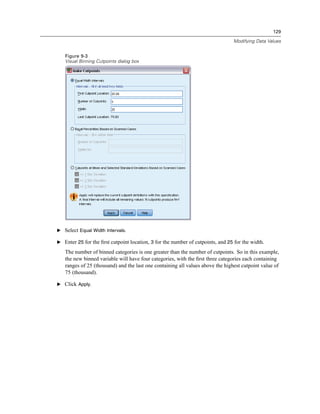
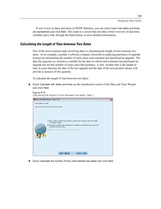
![137
Modifying Data Values
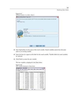
Figure 9-10
If Cases dialog box
E Select Include if case satisfies condition.
E Enter the conditional expression.
Most conditional expressions contain at least one relational operator, as in:
age>=21
or
income*3<100
In the first example, only cases with a value of 21 or greater for Age [age] are selected. In the
second example, Household income in thousands [income] multiplied by 3 must be less than
100 for a case to be selected.
You can also link two or more conditional expressions using logical operators, as in:
age>=21 | ed>=4
or
income*3<100 & ed=5
In the first example, cases that meet either the Age [age] condition or the Level of education [ed]
condition are selected. In the second example, both the Household income in thousands [income]
and Level of education [ed] conditions must be met for a case to be selected.](https://image.slidesharecdn.com/paswstatistics18briefguide-121129031530-phpapp02/85/Pasw-statistics-18-brief-guide-147-320.jpg)
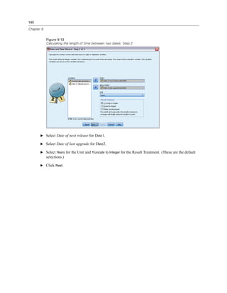

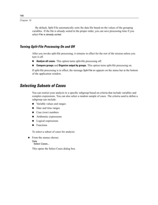
![Chapter
10
Sorting and Selecting Data
Data files are not always organized in the ideal form for your specific needs. To prepare data for
analysis, you can select from a wide range of file transformations, including the ability to:
Sort data. You can sort cases based on the value of one or more variables.
Select subsets of cases. You can restrict your analysis to a subset of cases or perform
simultaneous analyses on different subsets.
The examples in this chapter use the data file demo.sav. For more information, see the topic
Sample Files in Appendix A on p. 154.
Sorting Data
Sorting cases (sorting rows of the data file) is often useful and sometimes necessary for certain
types of analysis.
To reorder the sequence of cases in the data file based on the value of one or more sorting
variables:
E From the menus choose:
Data
Sort Cases...
The Sort Cases dialog box is displayed.
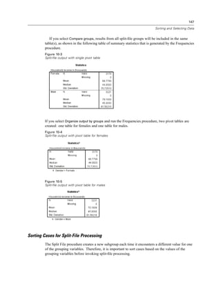
Figure 10-1
Sort Cases dialog box
E Add the Age in years [age] and Household income in thousands [income] variables to the Sort
by list.
145](https://image.slidesharecdn.com/paswstatistics18briefguide-121129031530-phpapp02/85/Pasw-statistics-18-brief-guide-155-320.jpg)
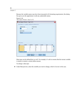
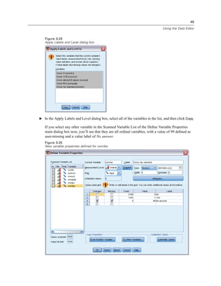
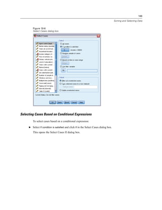
![146
Chapter 10
If you select multiple sort variables, the order in which they appear on the Sort by list determines
the order in which cases are sorted. In this example, based on the entries in the Sort by list, cases
will be sorted by the value of Household income in thousands [income] within categories of Age
in years [age]. For string variables, uppercase letters precede their lowercase counterparts in sort
order (for example, the string value Yes comes before yes in the sort order).
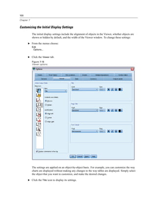
Split-File Processing
To split your data file into separate groups for analysis:
E From the menus choose:
Data
Split File...
The Split File dialog box is displayed.
Figure 10-2
Split File dialog box
E Select Compare groups or Organize output by groups. (The examples following these steps show
the differences between these two options.)
E Select Gender [gender] to split the file into separate groups for these variables.
You can use numeric, short string, and long string variables as grouping variables. A separate
analysis is performed for each subgroup that is defined by the grouping variables. If you
select multiple grouping variables, the order in which they appear on the Groups Based on list
determines the manner in which cases are grouped.](https://image.slidesharecdn.com/paswstatistics18briefguide-121129031530-phpapp02/85/Pasw-statistics-18-brief-guide-156-320.jpg)
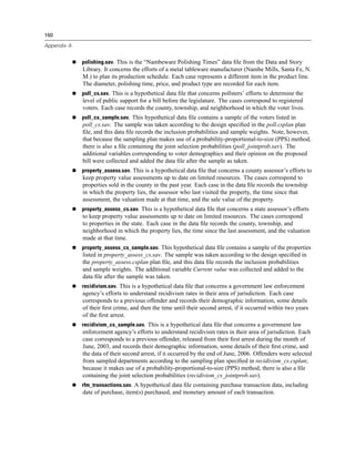
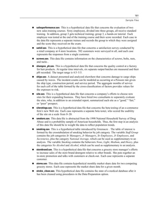
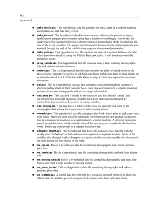
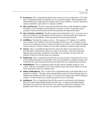

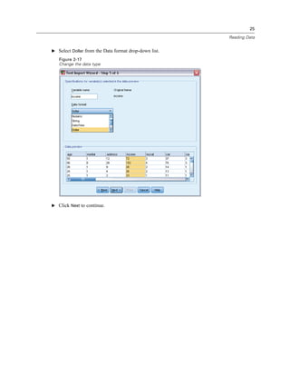
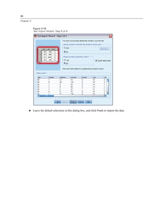
This document provides an overview and instructions for using PASW Statistics 18 software. It includes information about sample files, opening and reading data, running analyses, viewing results, and creating charts. Tutorials are provided for key tasks like entering data, defining variable properties, and reading data from different sources like spreadsheets, databases and text files. Technical support contact information and details regarding options, training and publications that complement the software are also summarized.