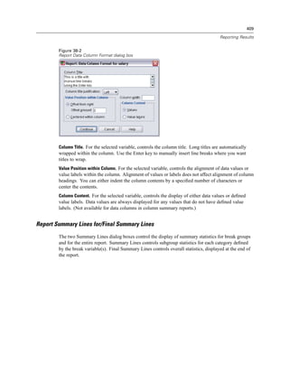
SPSS 16.0 is a software for statistical analysis that can analyze data from various sources and generate reports, charts, descriptive statistics, and complex statistical analyses. It includes procedures for regression, advanced models, tables, time series analysis, and more. The manual describes the graphical user interface of SPSS 16.0 Base and additional options are available as add-ons. Customer support and training is available from SPSS.


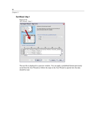
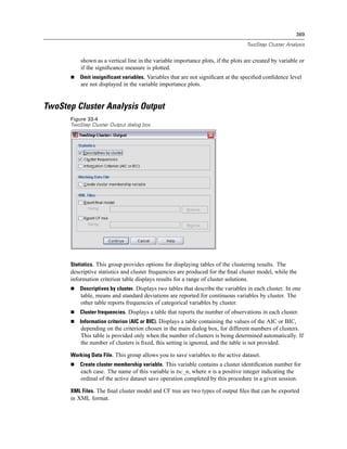
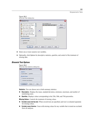
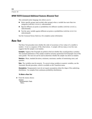
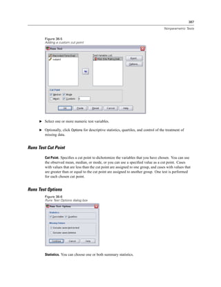
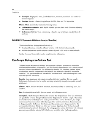
![20
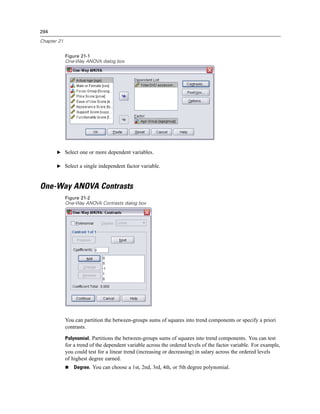
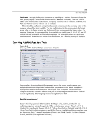
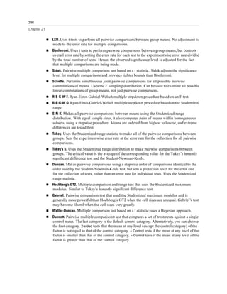
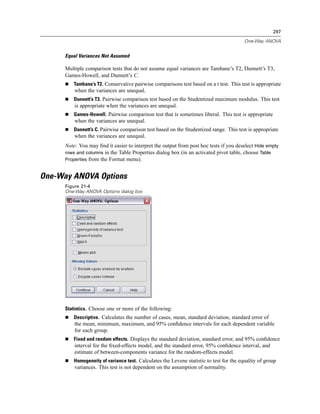
Chapter 3
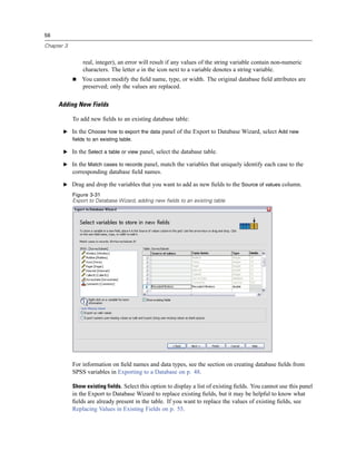
This takes you back to the first screen of the Database Wizard, where you can select the saved
name from the list of OLE DB data sources and continue to the next step of the wizard.
Deleting OLE DB Data Sources
To delete data source names from the list of OLE DB data sources, delete the UDL file with the
name of the data source in:
[drive]:Documents and Settings[user login]Local SettingsApplication DataSPSSUDL
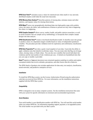
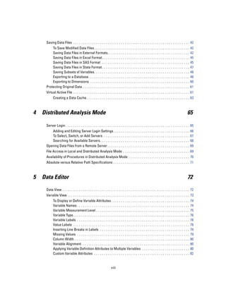
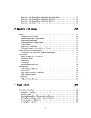
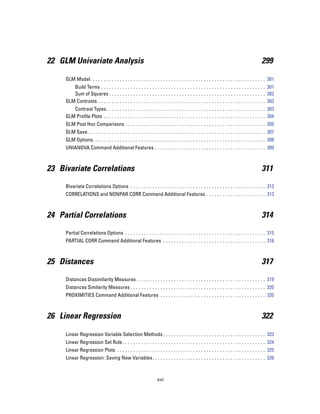
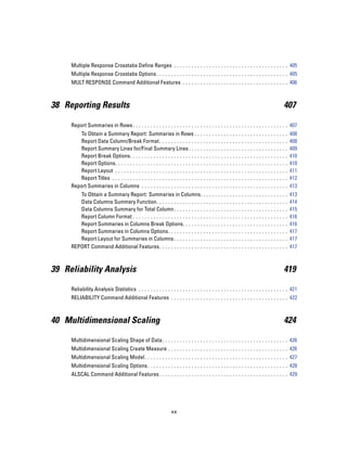
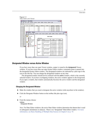
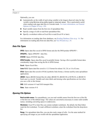
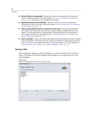
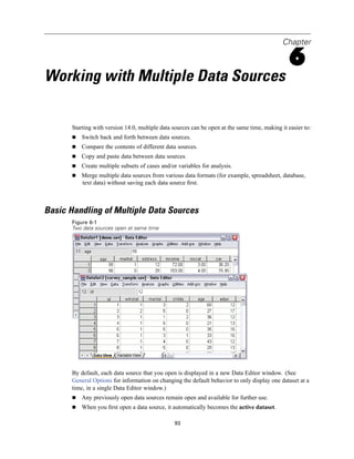
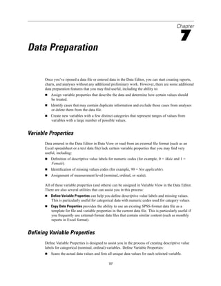
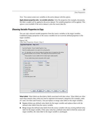
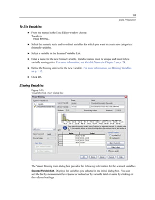
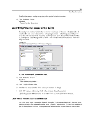
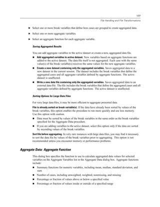
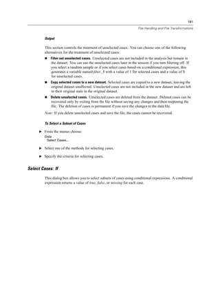
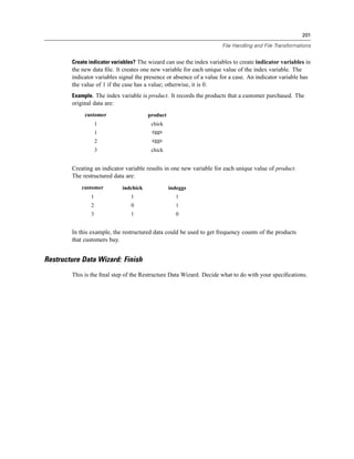
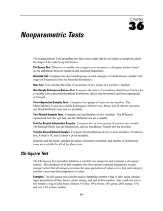
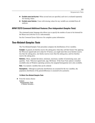
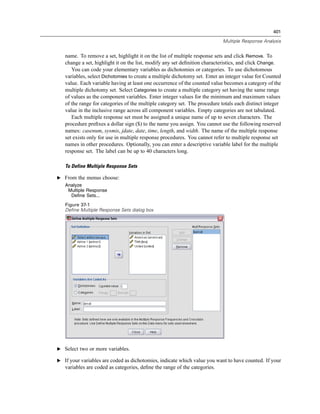
Selecting Data Fields
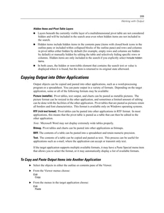
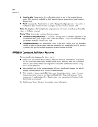
The Select Data step controls which tables and fields are read. Database fields (columns) are
read as variables.
If a table has any field(s) selected, all of its fields will be visible in the following Database
Wizard windows, but only fields that are selected in this step will be imported as variables. This
enables you to create table joins and to specify criteria by using fields that you are not importing.
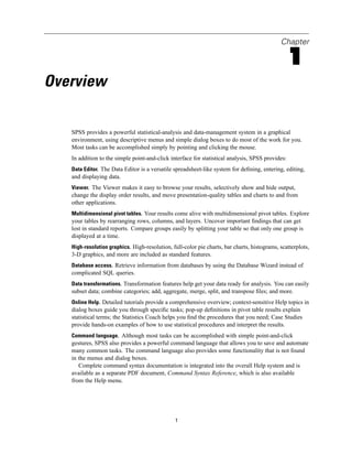
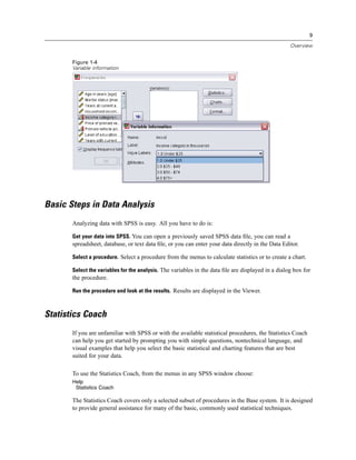
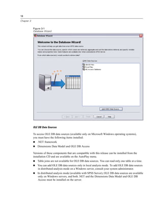
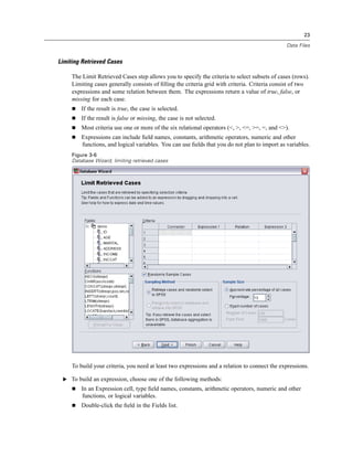
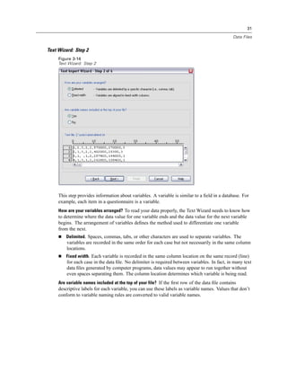
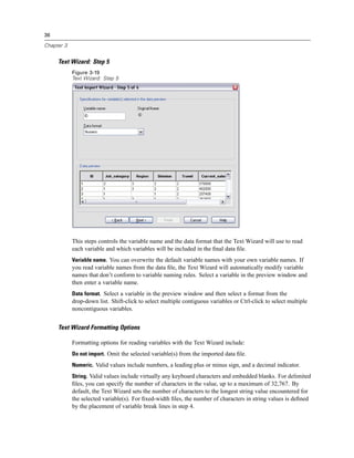
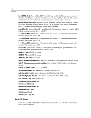
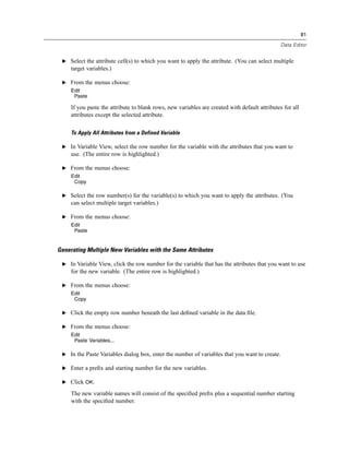
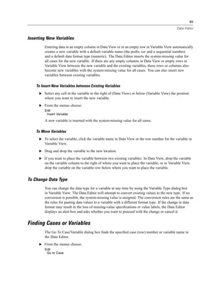
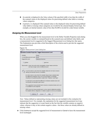
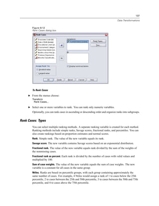
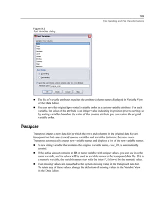
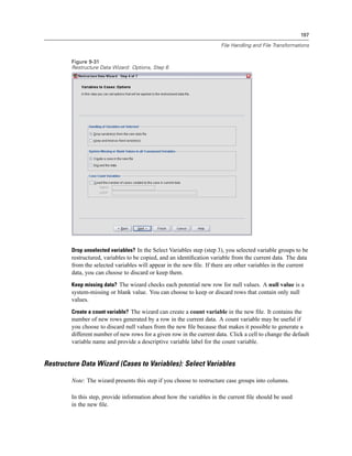
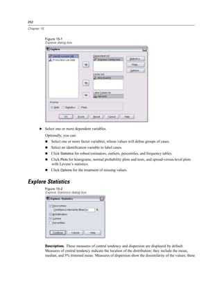
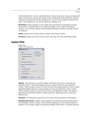
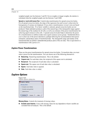
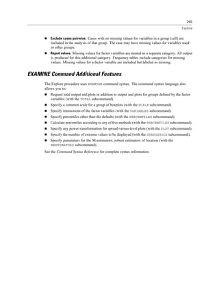
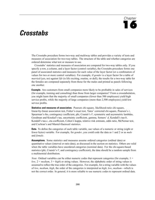
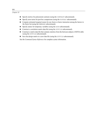
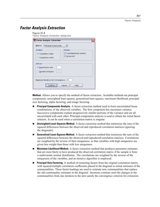
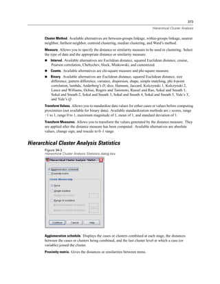
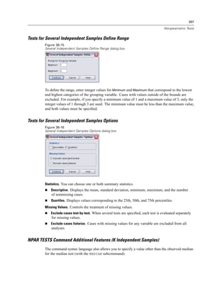
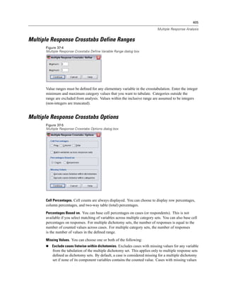
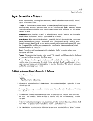
Figure 3-4
Database Wizard, selecting data
Displaying field names. To list the fields in a table, click the plus sign (+) to the left of a table name.
To hide the fields, click the minus sign (–) to the left of a table name.](https://image.slidesharecdn.com/spssbaseusersguide160-110501031823-phpapp02/85/Spss-base-users-guide160-44-320.jpg)

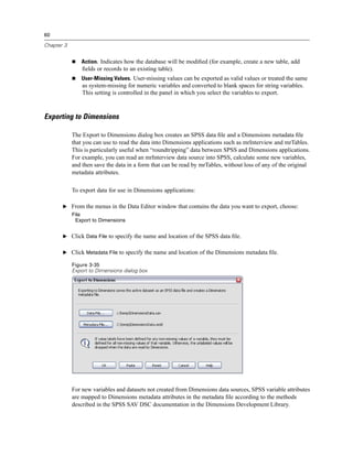
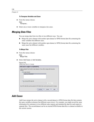
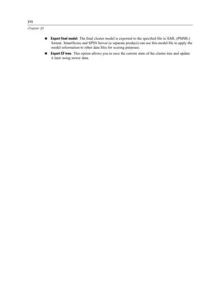
![70
Chapter 4
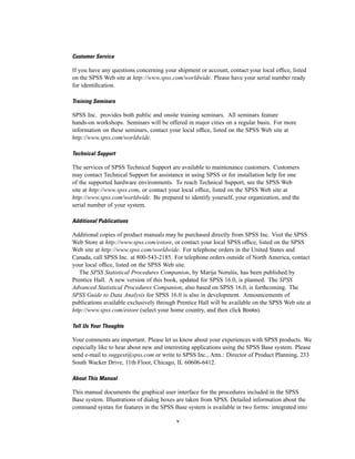
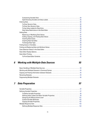
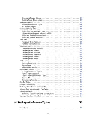
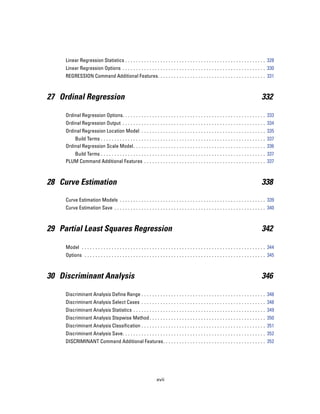
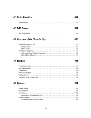
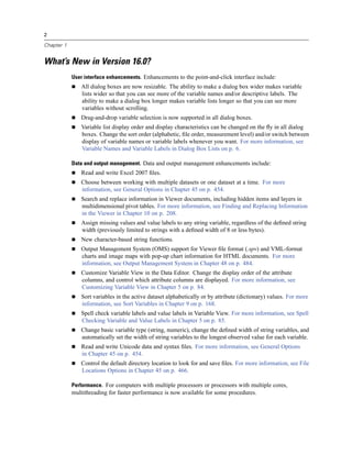
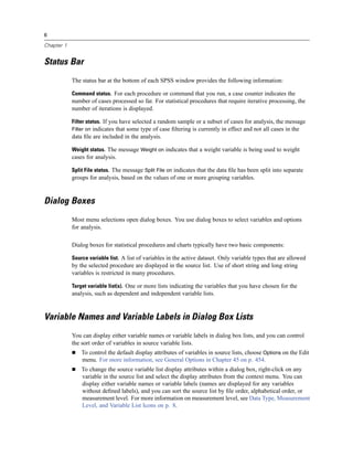
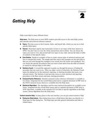
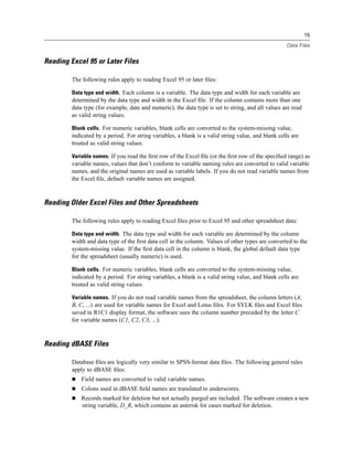
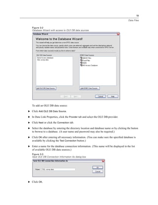
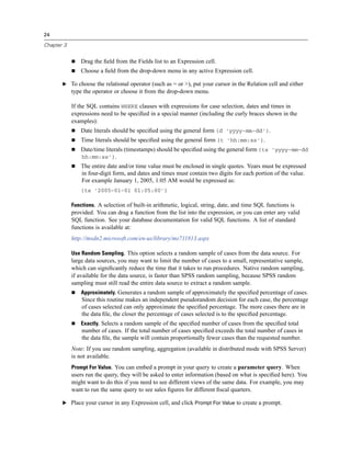
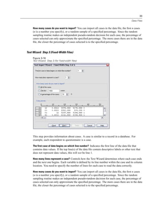
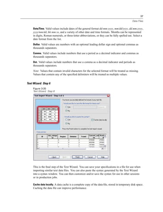
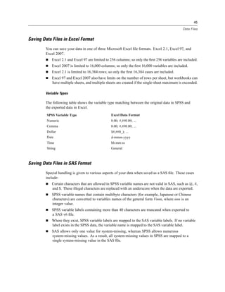
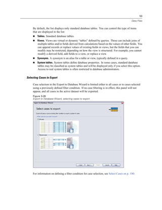
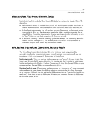
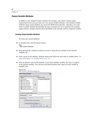
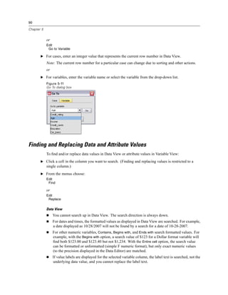
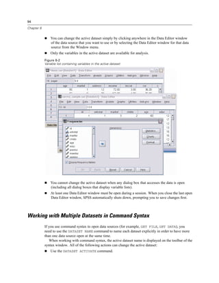
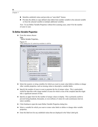
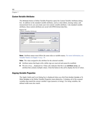
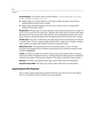
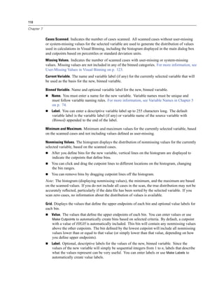
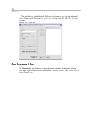
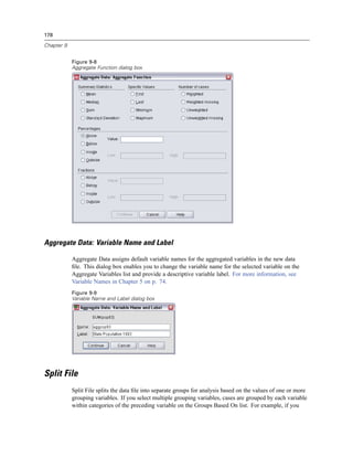
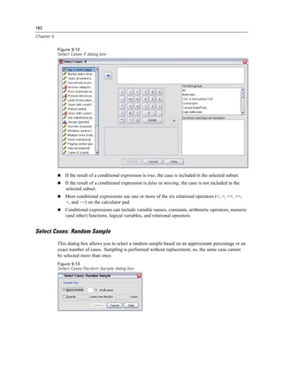
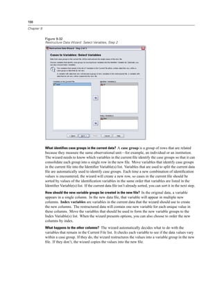
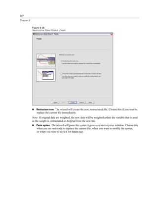
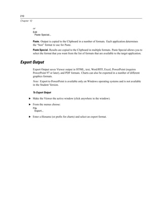
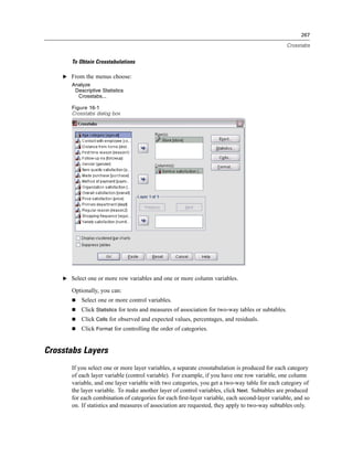
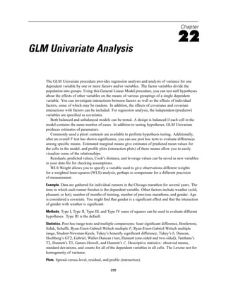
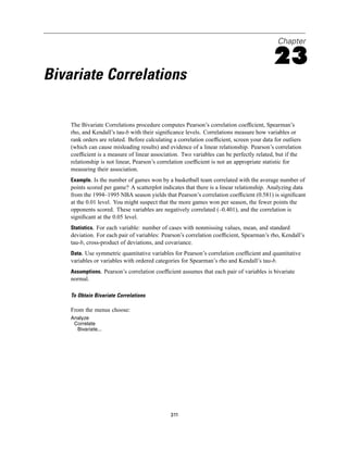
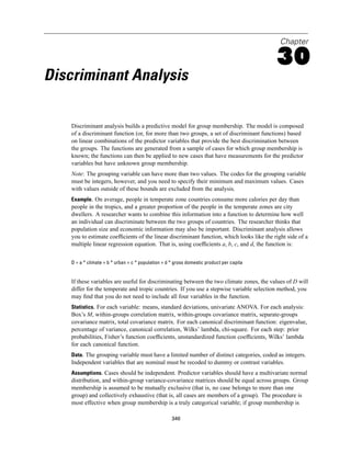
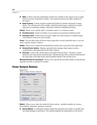
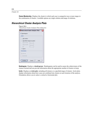
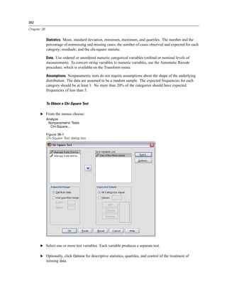
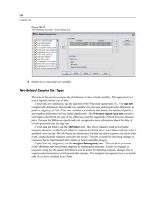
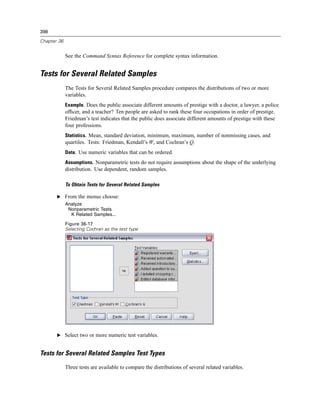
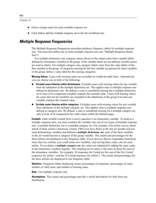
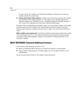
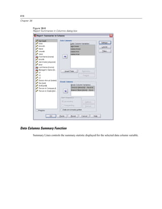
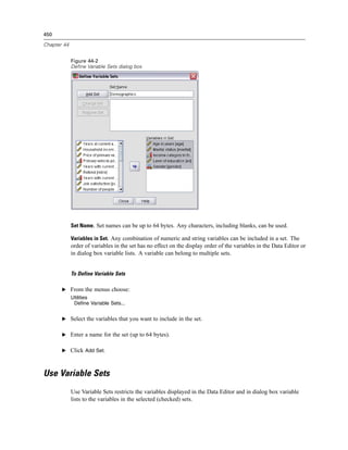
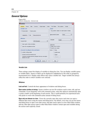
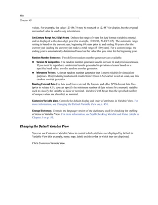
Figure 4-4
Local and remote views
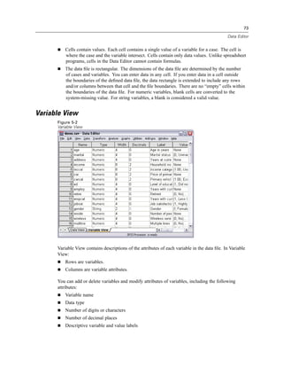
Local View
Remote View
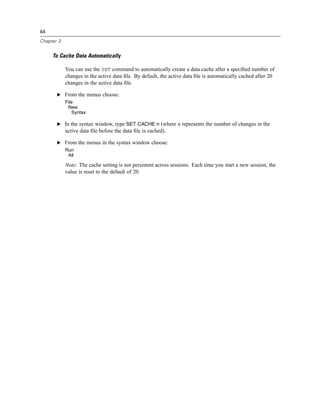
In distributed analysis mode, you will not have access to data files on your local computer unless
you specify the drive as a shared device or specify the folders containing your data files as shared
folders. If the server is running a different operating system (for example, you are running
Windows and the server is running UNIX), you probably won’t have access to local data files
in distributed analysis mode even if they are in shared folders.
Distributed analysis mode is not the same as accessing data files that reside on another
computer on your network. You can access data files on other network devices in local analysis
mode or in distributed analysis mode. In local mode, you access other devices from your local
computer. In distributed mode, you access other network devices from the remote server.
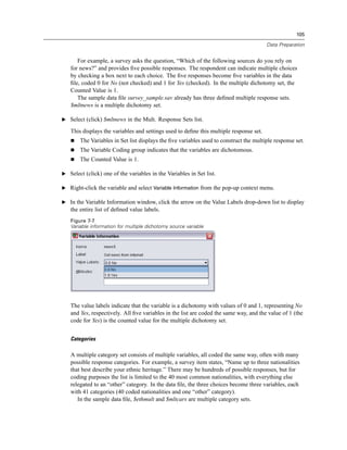
If you’re not sure if you’re using local analysis mode or distributed analysis mode, look at the
title bar in the dialog box for accessing data files. If the title of the dialog box contains the word
Remote (as in Open Remote File), or if the text Remote Server: [server name] appears at the top of
the dialog box, you’re using distributed analysis mode.
Note: This situation affects only dialog boxes for accessing data files (for example, Open Data,
Save Data, Open Database, and Apply Data Dictionary). For all other file types (for example,
Viewer files, syntax files, and script files), the local view is always used.
Availability of Procedures in Distributed Analysis Mode
In distributed analysis mode, procedures are available for use only if they are installed on both
your local version and the version on the remote server.
If you have optional components installed locally that are not available on the remote server
and you switch from your local computer to a remote server, the affected procedures will be
removed from the menus and the corresponding command syntax will result in errors. Switching
back to local mode will restore all affected procedures.](https://image.slidesharecdn.com/spssbaseusersguide160-110501031823-phpapp02/85/Spss-base-users-guide160-94-320.jpg)
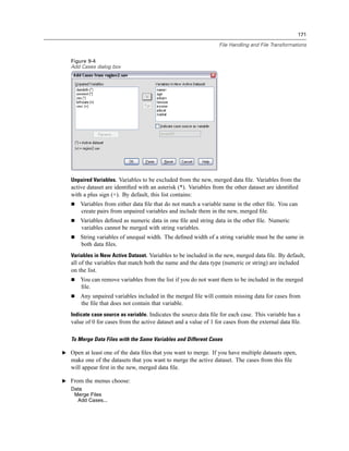
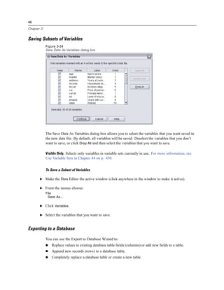
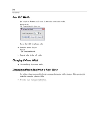
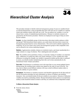
![229
Pivot Tables
Categories, including the label cell and data cells in a row or column
Category labels (without hiding the data cells)
Footnotes, titles, and captions
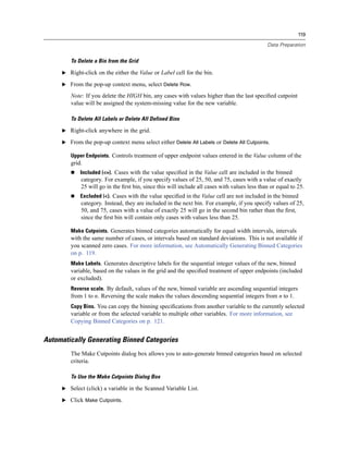
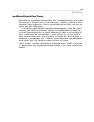
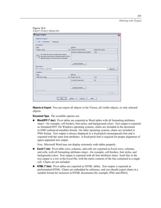
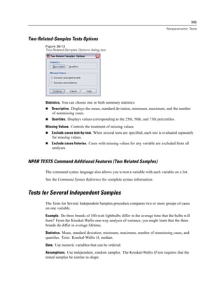
Hiding Rows and Columns in a Table
E Right-click the category label for the row or column you want to hide.
E From the context menu choose:
Select
Data and Label Cells
E Right-click the category label again and from the context menu choose Hide Category.
or
E From the View menu choose Hide.
Showing Hidden Rows and Columns in a Table
E Right-click another row or column label in the same dimension as the hidden row or column.
E From the context menu choose:
Select
Data and Label Cells
E From the menus choose:
View
Show All Categories in [dimension name]
or
E To display all hidden rows and columns in an activated pivot table, from the menus choose:
View
Show All
This displays all hidden rows and columns in the table. (If Hide empty rows and columns is selected
in Table Properties for this table, a completely empty row or column remains hidden.)
Hiding and Showing Dimension Labels
E Select the dimension label or any category label within the dimension.
E From the View menu or the context menu choose Hide Dimension Label or Show Dimension Label.
Hiding and Showing Table Titles
To hide a title:
E Select the title.
E From the View menu choose Hide.](https://image.slidesharecdn.com/spssbaseusersguide160-110501031823-phpapp02/85/Spss-base-users-guide160-253-320.jpg)
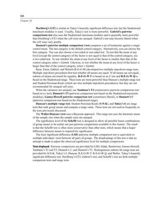

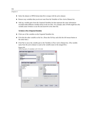
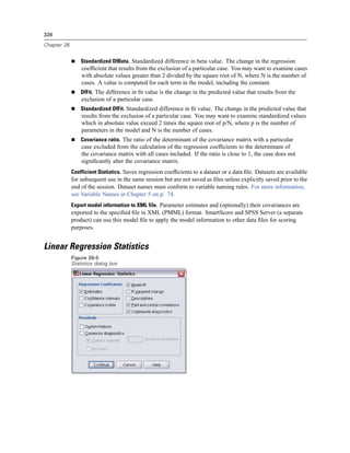
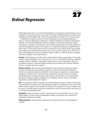
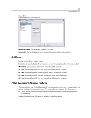
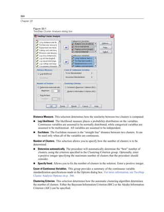
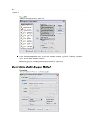
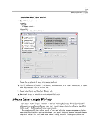
![327
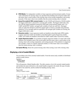
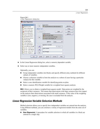
Linear Regression
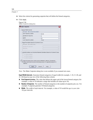
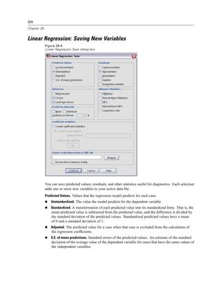
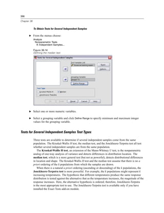
Distances. Measures to identify cases with unusual combinations of values for the independent
variables and cases that may have a large impact on the regression model.
Mahalanobis. A measure of how much a case’s values on the independent variables differ from
the average of all cases. A large Mahalanobis distance identifies a case as having extreme
values on one or more of the independent variables.
Cook’s. A measure of how much the residuals of all cases would change if a particular case
were excluded from the calculation of the regression coefficients. A large Cook’s D indicates
that excluding a case from computation of the regression statistics changes the coefficients
substantially.
Leverage values. Measures the influence of a point on the fit of the regression. The centered
leverage ranges from 0 (no influence on the fit) to (N-1)/N.
Prediction Intervals. The upper and lower bounds for both mean and individual prediction intervals.
Mean. Lower and upper bounds (two variables) for the prediction interval of the mean
predicted response.
Individual. Lower and upper bounds (two variables) for the prediction interval of the dependent
variable for a single case.
Confidence Interval. Enter a value between 1 and 99.99 to specify the confidence level for the
two Prediction Intervals. Mean or Individual must be selected before entering this value.
Typical confidence interval values are 90, 95, and 99.
Residuals. The actual value of the dependent variable minus the value predicted by the regression
equation.
Unstandardized. The difference between an observed value and the value predicted by the
model.
Standardized. The residual divided by an estimate of its standard deviation. Standardized
residuals, which are also known as Pearson residuals, have a mean of 0 and a standard
deviation of 1.
Studentized. The residual divided by an estimate of its standard deviation that varies from
case to case, depending on the distance of each case’s values on the independent variables
from the means of the independent variables.
Deleted. The residual for a case when that case is excluded from the calculation of the
regression coefficients. It is the difference between the value of the dependent variable and
the adjusted predicted value.
Studentized deleted. The deleted residual for a case divided by its standard error. The
difference between a Studentized deleted residual and its associated Studentized residual
indicates how much difference eliminating a case makes on its own prediction.
Influence Statistics. The change in the regression coefficients (DfBeta[s]) and predicted values
(DfFit) that results from the exclusion of a particular case. Standardized DfBetas and DfFit values
are also available along with the covariance ratio.
DfBeta(s). The difference in beta value is the change in the regression coefficient that results
from the exclusion of a particular case. A value is computed for each term in the model,
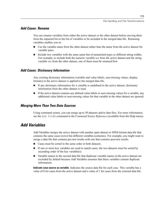
including the constant.](https://image.slidesharecdn.com/spssbaseusersguide160-110501031823-phpapp02/85/Spss-base-users-guide160-351-320.jpg)


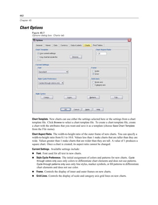
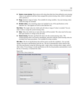
![482
Chapter 47
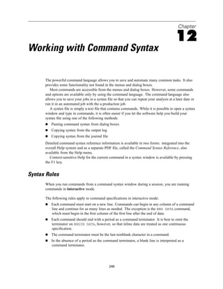
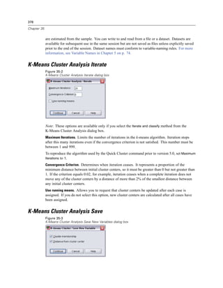
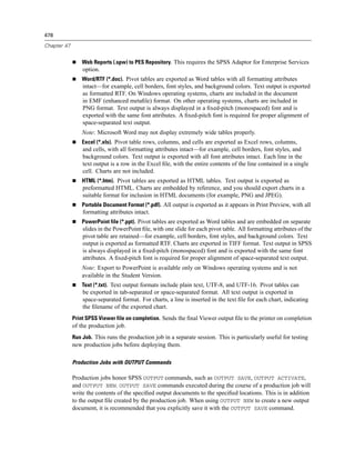
Running Production Jobs from a Command Line
Command line switches enable you to schedule production jobs to run automatically at certain
times, using scheduling utilities available on your operating system. The basic form of the
command line argument is:
spss filename.spj -production
Depending on how you invoke the production job, you may need to include directory paths for
the spss executable file (located in the directory in which the application is installed) and/or
the production job file.
You can run production jobs from a command line with the following switches:
-production [prompt|silent]. Start the application in production mode. The prompt and silent
keywords specify whether to display the dialog box that prompts for runtime values if they are
specified in the job. The prompt keyword is the default and shows the dialog box. The silent
keyword suppresses the dialog box. If you use the silent keyword, you can define the runtime
symbols with the -symbol switch. Otherwise, the default value is used. The -switchserver
and -singleseat switches are ignored when using the -production switch.
-symbol <values>. List of symbol-value pairs used in the production job. Each symbol name
starts with @. Values that contain spaces should be enclosed in quotes. Rules for including
quotes or apostrophes in string literals may vary across operating systems, but enclosing a
string that includes single quotes or apostrophes in double quotes usually works (for example,
“'a quoted value'”).
To run production jobs on a remote server in distributed analysis mode, you also need to specify
the server login information:
-server <inet:hostname:port>. The name or IP address and port number of the server. Windows only.
-user <name>. A valid user name. If a domain name is required, precede the user name with the
domain name and a backslash (). Windows only.
-password <password>. The user’s password. Windows only.
Example
spss production_jobsprodjob1.spj -production silent -symbol @datafile /data/July_data.sav
This example assumes that you are running the command line from the installation directory,
so no path is required for the spss executable file.
This example also assumes that the production job specifies that the value for @datafile should
be quoted (Quote Value checkbox on the Runtime Values tab), so no quotes are necessary
when specifying the data file on the command line. Otherwise, you would need to specify
something like "'/data/July_data.sav'" to include quotes with the data file specification, since
file specifications should be quoted in command syntax.
The directory path for the location of the production job uses the Windows back slash
convention. On Macintosh and Linux, use forward slashes. The forward slashes in the quoted
data file specification will work on all operating systems since this quoted string is inserted](https://image.slidesharecdn.com/spssbaseusersguide160-110501031823-phpapp02/85/Spss-base-users-guide160-506-320.jpg)
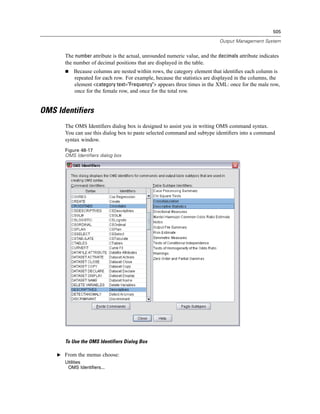
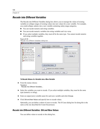
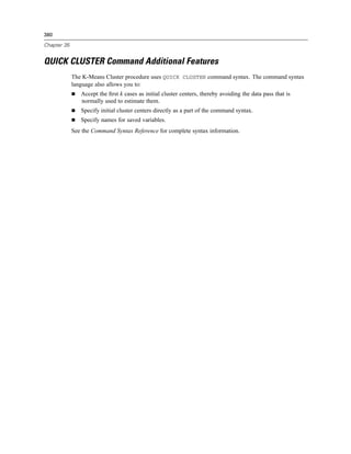
![506
Chapter 48
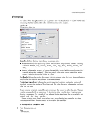
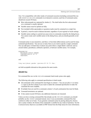
E Select one or more command or subtype identifiers. (Use Ctrl+click to select multiple identifiers
in each list.)
E Click Paste Commands and/or Paste Subtypes.
The list of available subtypes is based on the currently selected command(s). If multiple
commands are selected, the list of available subtypes is the union of all subtypes that are
available for any of the selected commands. If no commands are selected, all subtypes are
listed.
The identifiers are pasted into the designated command syntax window at the current
cursor location. If there are no open command syntax windows, a new syntax window
is automatically opened.
Each command and/or subtype identifier is enclosed in quotation marks when pasted, because
OMS command syntax requires these quotation marks.
Identifier lists for the COMMANDS and SUBTYPES keywords must be enclosed in brackets, as in:
/IF COMMANDS=['Crosstabs' 'Descriptives']
SUBTYPES=['Crosstabulation' 'Descriptive Statistics']
Copying OMS Identifiers from the Viewer Outline
You can copy and paste OMS command and subtype identifiers from the Viewer outline pane.
E In the outline pane, right-click the outline entry for the item.
E Choose Copy OMS Command Identifier or Copy OMS Table Subtype.
This method differs from the OMS Identifiers dialog box method in one respect: The copied
identifier is not automatically pasted into a command syntax window. The identifier is simply
copied to the clipboard, and you can then paste it anywhere you want. Because command and
subtype identifier values are identical to the corresponding command and subtype attribute values
in Output XML format (OXML), you might find this copy/paste method useful if you write
XSLT transformations.
Copying OMS Labels
Instead of identifiers, you can copy labels for use with the LABELS keyword. Labels can be used
to differentiate between multiple graphs or multiple tables of the same type in which the outline
text reflects some attribute of the particular output object, such as the variable names or labels.
There are, however, a number of factors that can affect the label text:
If split-file processing is on, split-file group identification may be appended to the label.
Labels that include information about variables or values are affected by the settings for the
display of variable names/labels and values/value labels in the outline pane (Edit menu,
Options, Output Labels tab).
Labels are affected by the current output language setting (Edit menu, Options, General tab).](https://image.slidesharecdn.com/spssbaseusersguide160-110501031823-phpapp02/85/Spss-base-users-guide160-530-320.jpg)
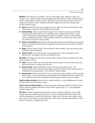
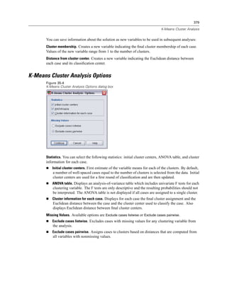
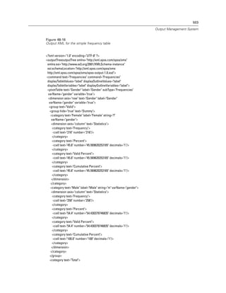
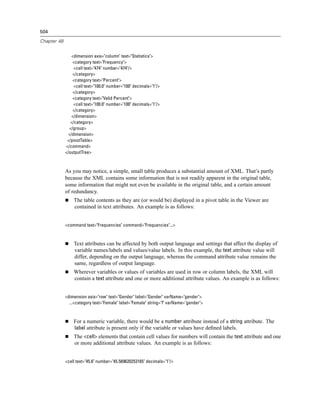
![507
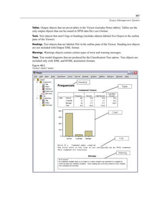
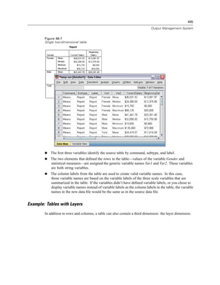
Output Management System
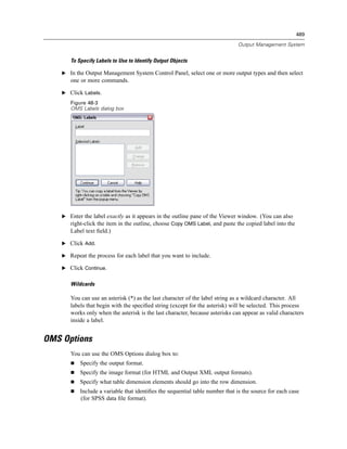
To copy OMS labels
E In the outline pane, right-click the outline entry for the item.
E Choose Copy OMS Label.
As with command and subtype identifiers, the labels must be in quotation marks, and the entire
list must be enclosed in square brackets, as in:
/IF LABELS=['Employment Category' 'Education Level']](https://image.slidesharecdn.com/spssbaseusersguide160-110501031823-phpapp02/85/Spss-base-users-guide160-531-320.jpg)