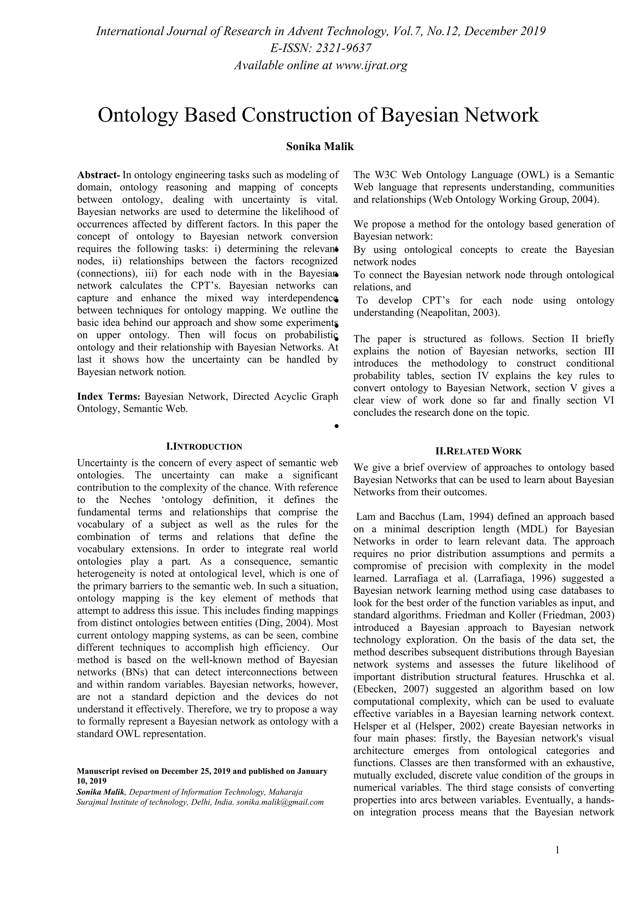
Ontology-based construction of Bayesian networks

International Journal of Research in Advent Technology, Vol.7, No.12, December 2019
E-ISSN: 2321-9637
Available online at www.ijrat.org
1
Ontology Based Construction of Bayesian Network
Sonika Malik
Abstract- In ontology engineering tasks such as modeling of
domain, ontology reasoning and mapping of concepts
between ontology, dealing with uncertainty is vital.
Bayesian networks are used to determine the likelihood of
occurrences affected by different factors. In this paper the
concept of ontology to Bayesian network conversion
requires the following tasks: i) determining the relevant
nodes, ii) relationships between the factors recognized
(connections), iii) for each node with in the Bayesian
network calculates the CPT’s. Bayesian networks can
capture and enhance the mixed way interdependence
between techniques for ontology mapping. We outline the
basic idea behind our approach and show some experiments
on upper ontology. Then will focus on probabilistic
ontology and their relationship with Bayesian Networks. At
last it shows how the uncertainty can be handled by
Bayesian network notion.
Index Terms: Bayesian Network, Directed Acyclic Graph
Ontology, Semantic Web.
I.INTRODUCTION
Uncertainty is the concern of every aspect of semantic web
ontologies. The uncertainty can make a significant
contribution to the complexity of the chance. With reference
to the Neches ‘ontology definition, it defines the
fundamental terms and relationships that comprise the
vocabulary of a subject as well as the rules for the
combination of terms and relations that define the
vocabulary extensions. In order to integrate real world
ontologies play a part. As a consequence, semantic
heterogeneity is noted at ontological level, which is one of
the primary barriers to the semantic web. In such a situation,
ontology mapping is the key element of methods that
attempt to address this issue. This includes finding mappings
from distinct ontologies between entities (Ding, 2004). Most
current ontology mapping systems, as can be seen, combine
different techniques to accomplish high efficiency. Our
method is based on the well-known method of Bayesian
networks (BNs) that can detect interconnections between
and within random variables. Bayesian networks, however,
are not a standard depiction and the devices do not
understand it effectively. Therefore, we try to propose a way
to formally represent a Bayesian network as ontology with a
standard OWL representation.
The W3C Web Ontology Language (OWL) is a Semantic
Web language that represents understanding, communities
and relationships (Web Ontology Working Group, 2004).
We propose a method for the ontology based generation of
Bayesian network:
• By using ontological concepts to create the Bayesian
network nodes
• To connect the Bayesian network node through ontological
relations, and
• To develop CPT’s for each node using ontology
understanding (Neapolitan, 2003).
•
• The paper is structured as follows. Section II briefly
explains the notion of Bayesian networks, section III
introduces the methodology to construct conditional
probability tables, section IV explains the key rules to
convert ontology to Bayesian Network, section V gives a
clear view of work done so far and finally section VI
concludes the research done on the topic.
•
II.RELATED WORK
We give a brief overview of approaches to ontology based
Bayesian Networks that can be used to learn about Bayesian
Networks from their outcomes.
Lam and Bacchus (Lam, 1994) defined an approach based
on a minimal description length (MDL) for Bayesian
Networks in order to learn relevant data. The approach
requires no prior distribution assumptions and permits a
compromise of precision with complexity in the model
learned. Larrafiaga et al. (Larrafiaga, 1996) suggested a
Bayesian network learning method using case databases to
look for the best order of the function variables as input, and
standard algorithms. Friedman and Koller (Friedman, 2003)
introduced a Bayesian approach to Bayesian network
technology exploration. On the basis of the data set, the
method describes subsequent distributions through Bayesian
network systems and assesses the future likelihood of
important distribution structural features. Hruschka et al.
(Ebecken, 2007) suggested an algorithm based on low
computational complexity, which can be used to evaluate
effective variables in a Bayesian learning network context.
Helsper et al (Helsper, 2002) create Bayesian networks in
four main phases: firstly, the Bayesian network's visual
architecture emerges from ontological categories and
functions. Classes are then transformed with an exhaustive,
mutually excluded, discrete value condition of the groups in
numerical variables. The third stage consists of converting
properties into arcs between variables. Eventually, a hands-
on integration process means that the Bayesian network
Manuscript revised on December 25, 2019 and published on January
10, 2019
Sonika Malik, Department of Information Technology, Maharaja
Surajmal Institute of technology, Delhi, India. sonika.malik@gmail.com

E-ISSN: 2321-9637
2
eliminates redundant arcs and state spaces. The approach
does not help visual form quantification (i.e. tables with the
conditional probability). Ding et al (Ding, 2004) suggest
probabilistic OWL mark-ups which can be applied in the
OWL ontology to individual’s classes and properties. The
authors described a sequence of rules to translate the OWL
ontology into DAG. CPT’s for the each network node are
built on the logical properties of its parent node. The
approach presented in this article contrasts with the existing
approaches:
• The graphic Bayesian Network Structure needs no special
extensions
• It is a common technique and a model for constructing
Bayesian networks on the basis of current OWL ontology.
• The necessary ontological extensions have no influence on
existing classes and ontological individuals.
III. BAYESIAN NETWORK
A Bayesian network of n parameters comprises of a direct
acyclic graph, which has n nodes and set of arcs as a whole.
Xi nodes equate to variables in a DAG, and direct arcs
between two nodes indicate a direct causal relationship
between one node and the other. The uncertainty of this
relationship is localized by CPT P (Xi | Пi) for each node Xi
where Пi is the parent set of Xi. At least in theory, BN
accepts some assumption in the mutual probability
distribution. Although the probabilistic inference with the
general structure of DAG has been shown to be NP-hard
(Cooper, 1990), BN inferential algorithms including belief
propagation (Pearl, 1986) and junction tree (Lauritzen,
1988) were developed for BN's causal structures for
successful calculation.
It is helpful to add some simple mathematical notation for
parameters and distributions of probabilities. The parameters
are shown with upper case letters (A, B, C) and lower case
letters (a, b, c) for their meanings. If A = a, they say A was
instantiated. The bold upper-cases letter (X) is a number of
variables and the bold lower-cases letter (x) is a specific set
of variables. If, for example, X indicates A, B, C then x is
the instantiation a, b, c. |X| is denoted as number of variables
in X. |A| is denoted as the number of possible states of a
discrete variable A. The parent of X in a graph is referred by
P(X). P (A) is used to denote the probability of A.
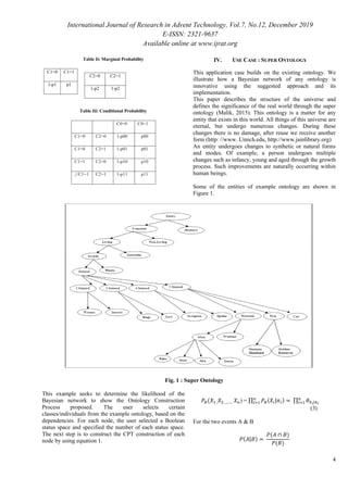
For the joint probability denotation P (A, B) and P (A|B) is
used and for conditional probability for the given variables
A & B. For e.g, if A is unambiguous, then P (A) may be
equal to states {0.2, 0.8} i.e. 20% chance of truth and 80%
chance of false. A joint probability means the likelihood of
the existence of more than one parameter, as A and B,
referred to as P (A, B).
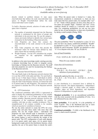
An example of joint probability distribution for variables
Raining and Windy is shown below in Table 1. For example,
the probability of it being windy and not raining is 0.28.
Table I: Joint Probability Distribution Example
Raining Wind=False Wind=True
True 0.1 0.9
False 0.72 0.28
The conditional probability is the likelihood of a variable,
given by another parameter, called (A|B). For example, the
probability of Windy being True, given that Raining is true
might equal 50%.
P (Windy = True | Raining = True) = 50%.
The whole theory of Bayesian network is based on Bayes
theorem that permits us to define the conditional probability
of evidence observing the cause based on the evidence.
P [Cause | Evidence] = P [Evidence | Cause] · P [Cause] P
[Evidence]
Each Bayesian network node is separate from its non-
descendants, provided that the parents have been in the
node. As Bayesian network is a function of probability, we
can use total likelihood as the criterion of statistical
knowledge. The highest probability estimation is a process
that calculates values for model parameters. The parameter
values are calculated so that the probability of the system as
defined by the model is maximized.
The benefit of the Bayesian network is that it handles
uncertainty in a tactful way as compare to other approaches.
A. Ontology Based construction of Bayesian network
For the development of Bayesian networks, the current
ontological method includes four major phases 1) select the
involved classes, individuals and properties, 2) Bayesian
Network Structure creation 3) Conditional probability Table
Creation 4) Inclusion of existing information
A. Select the involved classes, Individuals and Properties:
Every ontology class is well-defined, but a domain expert
must select those classes, individuals and properties that are
important to the problem considered and should be
represented within the Bayesian networks, although they are
semantically clear. Classes, individuals and properties are
relevant in this context as they affect the state of the final
output nodes of the Bayesian network (Fenz, 2012). The
domain expert must ensure that no redundant edges in the
Bayesian network are produced by selecting relevant
classes, individuals and properties. E.g. if A is influenced by
B and B by C only the edges of B to A, C to B are permitted.
The additional edge of C to A should not be permitted.
The domain expert has to select three different
class/individual types, 1) Node Class/Individual which is

E-ISSN: 2321-9637
3
directly related to problem domain 2) state space
class/individual that defines the node class/individual state
spaces 3) Weight Class/Individual define the node
classes/individual vector weights.
To build a Bayesian network, selection of nodes and state
space class is required.
• The number of potentials integrated into the Bayesian
network is constrained by the choice of groups and
individuals in the previous step. We use the category /
classes previously defined to identify four various types
of property for the building of Bayesian networks.
• Link Properties are those that connect the
class/individual of the node selected in the previous
step.
• State Value properties are those that provide the
numerical values for discrete states defined by state
space classes that are mutually exclusive.
• Weight Property: For the CPT calculation the weights
are required for the appropriate child-parent
combination.
In addition to the static knowledge model, ontology provides
a dynamic knowledge base in order to integrate current
knowledge as findings into the Bayesian network. The node
and class properties are used for incorporating the findings
in the Bayesian network.
B. Bayesian Network Structure creation
This step finally leads to the Bayesian network structure that
is to say that a DAG with nodes and links. For each built-in
node we use 1) State Space Classes / Individuals to define
node state space and allocate numerical values for each state
using the State Value Property selected, 2) Connect the node
to its parent nodes by link Properties. The numerical values
are required to calculate the CPTs of the Bayesian network
nodes.
C. CPT Construction
The conditional probability table (CPT) is represented in
order to display the conditional probabilities of one variable
relative to others for a set of linear and mutually reliant
random variables. Bayesian network inference involves the
computation of the conditional probability for certain
variables, with data on other variables (evidences). This is
straightforward if all evidence available is for variables
which are ancestral to variable(s) of interest.
We run the entire network to create the CPTs for every
related node and pick those nodes with more than null
parents. We use the weight classes / individuals and
properties for each selected node to determine its parent
nodes ' weights. For every child-parent node combination
the tertiary pattern is used to describe the weight of the
parent node. The CPT configuration of each node depends
on i) its parent node's state space, (ii) its parent node's
background weight and (iii) the distribution function, which
specifies the use of the parent States to decide the node's
state. When the parent node is limited to 2 states, the
measurement complexity is minimized, i.e. there are two
node states that have parent nodes, for example either “yes”
or “no”. Nodes without parents can have more than one or
two states, for example “high”, “medium” and “low”. Every
condition should be related to a numerical value lowest
state. For computing probabilities we can use two laws
either by law of total probability or chain rule of probability
by taking a small example (Zhang, 2009).
The prior probability ”P(A)” be attached to a class ”A” if it
does not have any parent, conditional probability ”P(A|B)”
be attached to a class ”A” if it is a subclass of class ”B” (so,
P(A|B)=0), and if necessary ”P(A|B)” are attached to a class
”A” if it is disjoint with class ”B” (so, P(A|B)=0)
Law of Total Probability
P (A) = Σ B P (A, B) = Σ B P (A | B) P (B)
(1)
Where B is any random variable
➢ Chain Rule Of Probabilities
We can also write
P (A, B, C… Z) = P (A | B, C… Z) P (B, C … Z) (by
definition of joint probability) (2)
Repeatedly applying this idea, we can write
P (A, B, C … Z) = P (A | B, C… Z) P (B | C... Z) P (C|...
Z)…P (Z)
A joint distribution in a structured form is defined by
Bayesian network. This depicts dependency / independence
through a directed graph, in which nodes are random
variables, edges are direct dependency and dependent
relations of independence as graph structure.
Marginal probability: It is an unconditional probability
with the event occurred with the probability (P (A)). It is
not influenced by any other event.
Joint probability: P (A and B). It is the probability of
event A and B. This is the likelihood that two or more
things will intersect. It can be written as P (A ∩ B).
Conditional probability: P (A|B) is the likelihood of the
event A, when event B is present.
A B C

E-ISSN: 2321-9637
4
Table Ii: Marginal Probability
C1=0 C1=1
1-p1 p1
Table Iii: Conditional Probability
C0=0 C0=1
C1=0 C2=0 1-p00 p00
C1=0 C2=1 1-p01 p01
C1=1 C2=0 1-p10 p10
;//C1=1 C2=1 1-p11 p11
IV. USE CASE : SUPER ONTOLOGY
This application case builds on the existing ontology. We
illustrate how a Bayesian network of any ontology is
innovative using the suggested approach and its
implementation.
This paper describes the structure of the universe and
defines the significance of the real world through the super
ontology (Malik, 2015). This ontology is a matter for any
entity that exists in this world. All things of this universe are
eternal, but undergo numerous changes. During these
changes there is no damage, after reuse we receive another
form (http: //www. Umich.edu, http://www.jainlibrary.org)
An entity undergoes changes to synthetic or natural forms
and modes. Of example, a person undergoes multiple
changes such as infancy, young and aged through the growth
process. Such improvements are naturally occurring within
human beings.
Some of the entities of example ontology are shown in
Figure 1.
Fig. 1 : Super Ontology
This example seeks to determine the likelihood of the
Bayesian network to show the Ontology Construction
Process proposed. The user selects certain
classes/individuals from the example ontology, based on the
dependencies. For each node, the user selected a Boolean
status space and specified the number of each status space.
The next step is to construct the CPT construction of each
node by using equation 1.
𝑃𝐵(𝑋1 , 𝑋2 ,……, 𝑋 𝑛) = ∏ 𝑃𝐵( 𝑋𝑖|𝜋𝑖) = ∏ 𝜃 𝑋 𝑖|𝜋 𝑖
𝑛
𝑖=1
𝑛
𝑖=1
(3)
For the two events A & B
𝑃( 𝐴|𝐵) =
𝑃(𝐴 ∩ 𝐵)
𝑃(𝐵)
C2=0 C2=1
1-p2 1-p2

E-ISSN: 2321-9637
5
𝑃( 𝐵|𝐴) =
𝑃(𝐴 ∩ 𝐵)
𝑃(𝐴)
𝑃( 𝐴|𝐵) 𝑃( 𝐵) = 𝑃( 𝐴 ∩ 𝐵) = 𝑃( 𝐵|𝐴) 𝑃(𝐴)
P(A|B) =
𝑃( 𝐵| 𝐴)𝑃(𝐴)
𝑃(𝐵)
CPT for the node Animal with all its sub-classes like 2-
sensed, 3-sensed, 4-sensed and so on as given in the Table 4.
TABLE IVA: CPT FOR ANIMAL WITH 2-SENSED
Animal 2-sensed
True False
True 0.6 0.4
False 0 1
TABLE IVB: CPT FOR ANIMAL WITH 3-SENSED
Animal 3-sensed
True False
True 0.75 0.25
False 0 1
TABLE IVC: CPT FOR ANIMAL WITH 4-SENSED
Animal 4-sensed
True False
True 0.89 0.11
False 0 1
TABLE IVD: CPT FOR ANIMAL WITH 5-SENSED
Animal 5-sensed
True False
True 0.95 0.05
False 0 1
Now for the next level the CPT for each node is given in
Table 5.
TABLE VA: CPT FOR 2-SENSED WITH WORMS
Animal 2
sensed
Worms
True False
True True 0.5 0.5
True False 0.05 0.95
False True 0 1
False False 0 1
TABLE VB: CPT FOR 2-SENSED WITH INSECTS
Animal 2
sensed
Insects
True False
True True 0.5 0.5
False True 0 1
False False 0 1
There can be 2-sensed Animals like worms and insects and
if the animals are not 2-sensed the n there is very less
probablity that they are worms or insects. Similarly for 3-
sensed, 4-sensed and 5-sensed animals.
TABLE VC: CPT FOR 3-SENSED WITH BUGS
Animal 3-
sensed
Bugs
True False
True True 0.5 0.5
False True 0 1
False False 0 1
TABLE VD: CPT FOR 3-SENSED WITH LICE
Animal 3-
sensed
Lice
True False
True True 0.55 0.45
False True 0 1
False False 0 1
TABLE VE: CPT FOR 4-SENSED WITH SCORPIO
Animal 4-
sensed
Scorpio
True False
True True 0.85 0.15
False True 0 1
False False 0 1
TABLE VF: CPT FOR 4-SENSED WITH SPIDER
Animal 4-
sensed
Spider
True False
True True 0.5 0.5
False True 0 1
False False 0 1
TABLE VG: CPT FOR 5-SENSED WITH HUMAN
Animal 4-
sensed
Human
True False
True True 0.99 0.01
True False 0.4 0.6
False True 0 1
False False 0 1
TABLE VH: CPT FOR 5-SENSED WITH CAT
Animal 5
sensed
Cat
True False
True True 0.55 0.45
False True 0 1
False False 0 1

E-ISSN: 2321-9637
6
Table VIA: CPT for 5-sensed with Dog
Animal 5
sensed
Dog
True False
True True 0.7 0.3
False True 0 1
False False 0 1
After this we will come to the next level and CPT for the
each node is given in Table 6.
TABLE VIB: CPT FOR 5-SENSED WITH HUMAN WITH MAN
Animal 5 sense Human Man
True False
True True True 0.87 0.13
True True False 0.3 0.7
True False True 0.65 0.35
True False False 0.45 0.55
False True True 0 1
False True False 0 1
False False True 0 1
False False False 0 1
If 5 sensed animal is a human then it can either be Man or
Woman.
TABLE VIC: CPT FOR 5-SENSED WITH HUMAN WITH WOMAN
Animal 5 sense Human Woman
True False
False True True 0 1
TABLE VID: CPT FOR 5-SENSED WITH HUMAN WITH MAN
WITH RAM
Animal 5 sense Human Man Ram
True False
True True True True 0.97 0.03
True True True False 0.55 0.45
True True False True 0.2 0.8
True True False False 0.25 0.75
True False True True 0.63 0.27
True False True False 0.6 0.4
True False False True 0.35 0.65
True False False False 0.3 0.7
False True True True 0 1
False True True False 0 1
False True False True 0 1
False True False False 0 1
False False True True 0 1
False False True False 0 1
False False False True 0 1
False False False False 0 1
TABLE VIE: CPT FOR 5-SENSED WITH HUMAN WITH WOMAN
WITH SITA
Animal 5 sense Human Woman Sita
True False
True True True True 0.89 0.11
True True True False 0.4 0.6
True True False True 0.25 0.75
True True False False 0.42 0.58
True False True True 0.54 0.46
True False True False 0.61 0.39
rue False False True 0.4 0.6
True False False False 0.25 0.75
False True True True 0 1
False True True False 0 1
False True False True 0 1
False True False False 0 1
False False True True 0 1
False False True False 0 1
alse False False True 0 1
False False False False 0 1
TABLE VIF: CPT FOR 5-SENSED WITH DOG WITH ANY
SPECIES
Animal 5 sense Dog Any Species
True False
False True True 0 1
TABLE VIG: CPT FOR 5-SENSED WITH CAT WITH ANY
SPECIES
Animal 5 sense Cat Any Species
True False
False True True 0 1
After calculating all the probablities and CPT construction
the final step is to construct the bayesian network for the
existing ontology as in Figure 1. The translated Bayesian
network from the super ontology is shown in Figure 2.
The provided use case developed a core Bayesian network
of 120 nodes, 454 axioms and 119 links. It allows an expert
in the field to build a Bayesian network based on existing
ontology. The efficiency of the developed Bayesian network
is evaluated for the use case. The usefulness of constructing
bayesian network is i) It enabled them to build a bayesinan
network effectively without any external help., ii) the
information needed in ontology is centrally managed and
transferred to the bayesian network. Finally the building
steps for each node are: i) scanning the name of ontology

E-ISSN: 2321-9637
7
node and its type ii) state space include the allocation of
numerical value (for example “true” or “false”) iii) verifying
each node should be connected to the current node iv)
Linking of each node to its parent and its child.
Fig. 2: Translated BN for Super Ontology
V. CONCLUSION & FUTURE WORK
While creating the Bayesian Networks the following
challenges are faced: i) What variables are required for any
issue? ii) How to link these variables to each other? iii)
What are the states of the determined variables? To
overcome such problems, an ontology based approach for
developing Bayesian networks is introduced and
demonstrate its applicability for existing ontology. The
proposed method enables the creation of Bayesian networks
by giving the probablity at each node, which can handle
uncertainty also.
The limitations of this method is: Ontology does not
provide the functionsfor computing the CPT’s, it must be
explicitly modeled.
REFERENCES
[1] Z. Ding and Y. Peng, “A Probabilistic Extension to Ontology
Language OWL,” Proc. 37th Hawaii Int’l Conf. System Sciences
(HICSS 04), IEEE CS Press, 2004.
[2] http://www.w3.org/2004/OWL
[3] R. Neapolitan. Learning Bayesian networks. Prentice Hall, 2003.
[4] W. Lam, F. Bacchus, “Learning Bayesian belief networks: an
approach based on the mdl principle”, Computational Intelligence, vol
10, 1994. 269–293.
[5] P. Larrafiaga, C. Kuijpers, R. Murga, Y. Yurramendi, “Learning
Bayesian network structures by searching for the best ordering with
genetic algorithms”, IEEE Transactions on Systems, Man, and
Cybernetics — Part A 26, 1996 487–493.
[6] N. Friedman, D. Koller, “Being Bayesian about network structure. a
Bayesian approach to structure discovery in Bayesian networks”,
Machine Learning 50, 2003, 95–125.
[7] E.R.H. Jr., N.F. Ebecken, “Towards efficient variables ordering for
Bayesian networks classifier”, Data & Knowledge Engineering, vol
63 (2), 2007 258–269.
[8] E.M. Helsper, L.C. van der Gaag, Building Bayesian networks
through ontologies, in: F. van Harmelen (Ed.), ECAI 2002:
Proceedings of the 15th European Conference on Artificial
Intelligence, IOS Press, 2002, pp. 680–684.
[9] G. F. Cooper, “The computational complexity of probabilistic
inference using Bayesian belief network,” Artificial Intelligence, vol.
42, 1990, 393–405.
[10] J. Pearl, “Fusion, propagation and structuring in belief networks,”
Artificial Intelligence, vol. 29, 1986, 241–248.
[11] S. L. Lauritzen and D. J. Spiegelhalter, “Local computation with
a. Probabilities in graphic structures and their applications in expert
systems,” J. Royal Statistical Soc. Series B, vol. 50(2), 1988, 157–
224.
[12] S. Fenz. “An ontology-based approach for constructing Bayesian
networks”, Data & Knowledge Engineering, volume 73, 2012, 73–88.
[13] S. Zhang, Y. Sun, Y. Peng, X. Wang, BayesOWL: A Prototypes
System for Uncertainty in Semantic Web. In Proceedings of IC-AI,
678-684, 2009.
[14] S. Malik, S. Jain, “Sup_Ont:An upper ontology (Accepted for
Publication),” IJWLTT, IGI Global, to be published.
[15] http://www.umich.edu/~umjains/jainismsimplified/chapter03.html.
[16] http://www.jainlbrary.org/JAB/11_JAB_2015_Manual_Finpdf.
AUTHORS PROFILE
Sonika Malik has done B.Tech from Kurukshetra
University, India in 2004 and did her Masters from
MMU in 2010. She is doing her doctorate from
National Institute of technology, Kurukshetra. She
has served in the field of education from last 12 years
and is currently working at Maharaja Surajmal
Institute of Technology, Delhi. Her current research
interests are in the area of Sematic Web, Knowledge
representation and Ontology Design.

Ontology-based construction of Bayesian networks

Recommended

Recommended

More Related Content

What's hot

What's hot (18)

Similar to Ontology-based construction of Bayesian networks

Similar to Ontology-based construction of Bayesian networks (20)

More from IJRAT

More from IJRAT (20)

Recently uploaded

Recently uploaded (20)

Ontology-based construction of Bayesian networks