Downloaded 280 times


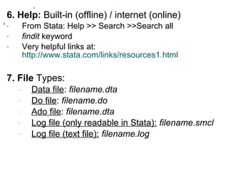


![10. Data manipulation
Creating new variables (gen) (cont’d)
gen l_income=log(income) //natural log
OR gen l_income=ln(income) //natural log
gen loginc=log10(income) //base 10 log
gen Y=sqrt(X) //get square-root of X
gen Z=exp(Y) //get the exponential
gen sqage=age^2 //get the square age
gen XY=X*Y //interaction term
gen lagYt = Yt[_n-1] //lagYt=Yt-1](https://image.slidesharecdn.com/pptstata-finalandcomplete-141017134736-conversion-gate01/85/Introduction-to-Stata-36-320.jpg)

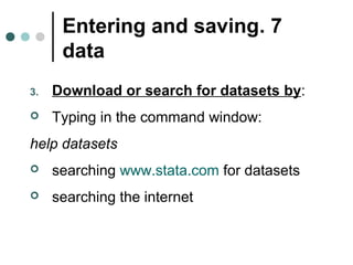
The document is a comprehensive overview of Stata software usage in social science research, detailing its interface, capabilities compared to SPSS, and various editions. It provides practical guidance on data manipulation, statistical analysis, graphics, and report preparation using Stata commands. Additionally, it includes best practices and tips for effectively managing and analyzing data within the software.