This document describes a master's thesis project focused on sensorless speed and position estimation of a permanent magnet synchronous machine (PMSM). The project investigates sensorless control strategies using a back electromotive force (Back-EMF) method for position estimation and a phase-locked loop (PLL) for speed estimation. A field oriented control (FOC) system is designed to control the PMSM. The objectives are to propose bandwidths for different operating states, investigate angular position estimation errors, and compensate for magnetic saturation effects. Simulation and experimental results are presented to evaluate the sensorless control strategy.

1. Sen sorlesssp eed
a n d p osition
estim a tion
Grou p :PE D 4-1064
A a lborg Un iversity
D ep a rtm en tofE n ergy Techn ology
Ju n e 3 ,2014

2. Title: Sensorless speed and position estimation of a PMSM
Semester: 4rd semester M.Sc., PED4
Semester theme: Master Thesis
Period: 17-02-2013 / 03-06-2014
ECTS: 30
Supervisor: Kaiyuan Lu and Hernan Miranda Delpino
Project group: PED4-1046
Cesar Hernaez
Copies: 2
Number of pages: 75
Appendix pages: 12
CD’s: 2
ABSTRACT:
This Project focuses on investigating the sen-
sorless speed and position estimation control
of a Surface Mounted Permanent Magnet Syn-
chronous Machine for medium and high speed,
proposing a bandwidth for different steady and
dynamic states and investigating about the an-
gular estimation position error. Back-EMF
method is used to estimate the position, and
Phase Loop Lock (PLL) method is used to es-
timate the speed. An Auto-tuning is designed
for both in order to achieve good performance
based on the bandwidth and the position error.
A field Oriented Control (FOC) system was de-
signed which is know to give good results and
good dynamic performance. A VSI controls the
machine currents using Space Vector Modula-
tion (SVM). First The literature is searched for
a suitable Back-EMF sensorless control method,
position error and bandwidth. Then the selected
best methods are implemented and tested in the
simulation. The overall selected control system
is tested in the laboratory setup and compare
the sensorless control strategy with the sensored
control.
By signing this document, each member of the group confirms that all participated in
the project work and thereby that all members are collectively liable for the content of
the report.
iii

3. Table of Contents
1 Introduction 1
1.1 Background . . . . . . . . . . . . . . . . . . . . . . . . . . . . . . . . . . . . . . . . . . 1
1.2 Problem statement . . . . . . . . . . . . . . . . . . . . . . . . . . . . . . . . . . . . . . 1
1.3 Objective . . . . . . . . . . . . . . . . . . . . . . . . . . . . . . . . . . . . . . . . . . . 2
1.4 Limitations and assumptions . . . . . . . . . . . . . . . . . . . . . . . . . . . . . . . . 2
2 System Description 3
2.1 System overview . . . . . . . . . . . . . . . . . . . . . . . . . . . . . . . . . . . . . . . 3
2.2 PMSM mathematical model . . . . . . . . . . . . . . . . . . . . . . . . . . . . . . . . . 6
2.3 Inverter . . . . . . . . . . . . . . . . . . . . . . . . . . . . . . . . . . . . . . . . . . . . 7
3 FOC control 9
3.1 Introduction . . . . . . . . . . . . . . . . . . . . . . . . . . . . . . . . . . . . . . . . . . 9
3.2 FOC Strategy . . . . . . . . . . . . . . . . . . . . . . . . . . . . . . . . . . . . . . . . . 9
3.3 Control design . . . . . . . . . . . . . . . . . . . . . . . . . . . . . . . . . . . . . . . . 11
3.4 Simulation and Experimental results . . . . . . . . . . . . . . . . . . . . . . . . . . . . 21
4 Sensorless Control 25
4.1 Introduction . . . . . . . . . . . . . . . . . . . . . . . . . . . . . . . . . . . . . . . . . . 25
4.2 Position estimation . . . . . . . . . . . . . . . . . . . . . . . . . . . . . . . . . . . . . . 26
4.3 Inductance compensation . . . . . . . . . . . . . . . . . . . . . . . . . . . . . . . . . . 34
4.4 Speed estimator . . . . . . . . . . . . . . . . . . . . . . . . . . . . . . . . . . . . . . . . 38
4.5 Control design . . . . . . . . . . . . . . . . . . . . . . . . . . . . . . . . . . . . . . . . 39
5 Sensorless Experimental results 47
5.1 Speed steps with no load. . . . . . . . . . . . . . . . . . . . . . . . . . . . . . . . . . . 47
5.2 Speed steps with constant load torque. . . . . . . . . . . . . . . . . . . . . . . . . . . . 50
5.3 Constant speed command with load torque steps. . . . . . . . . . . . . . . . . . . . . . 52
6 Conclusion 55
7 CD Content 57
Bibliography 59
Appendix A VSI modulation strategy I
Appendix B Back-EMF method III
v

4. List of Symbols
Symbol Description Units
fs dSPACE system sampling frequency Hz
fsw VSI switching frequency Hz
vab, vbc, vca Line-to-line voltages V
van, vbn, vcn Phase-to-neutral voltages V
vaN , vbN , vcN VSI leg voltages V
Sx VSI switch state value -
Vdc VSI DC link voltage V
vabcs Stator voltage vector V
iabcs Stator current vector A
Rs Stator resistance matrix Ω
Labcs Stator inductance matrix H
λabcs Total stator flux linkage Wb
λpmabcs Permanent magnet flux linkage vector Wb
v r
qs, v r
ds q- and d-axis voltages V
vα, vβ α- and β-axis voltages V
ir
qs, ir
ds q- and d-axis currents A
iα, iβ α- and β-axis currents A
Lq, Ld q- and d-axis inductances H
Lα, Lβ α- and β-axis inductances H
λα, λβ α- and β-axis flux linkage H
λq, λd q- and d-axis flux linkage H
Rs Stator resistance Ω
λαβ αβ flux linkage Wb
λdq dq flux linkage Wb
λpm Permanent magnet flux Wb
θr Electrical angular rotor position rad
θ Electrical angular rotor position rad
ωr Electrical angular speed rad/s
ω Electrical angular speed rad/s
θm Mechanical angular rotor position rad
ωm Mechanical angular speed rad/s
n Mechanical angular speed rpm
pp Number of polepairs -
Te Electromagnetic torque Nm
Tload Mechanical load torque Nm
Jm Combined inertia coefficient of PMSM and load kg·m2
Bm Combined viscous damping coefficient of PMSM and load Ns/m
J0 Combined coulomb friction coefficient of PMSM and load Nm
nm Mechanical shaft speed min−1
τ Time constant s
JPMSM Inertia coefficient of the PMSM kg·m2
JIM Inertia coefficient of the IM kg·m2
JCoupling Inertia coefficient of the coupling kg·m2
s Laplace variable -
vii

5. Symbol Description Units
Kp Controller proportional gain -
Ki Controller integral gain -
K1 Constant gain -
K1 Constant gain -
Td DSP system time delay s
G Transfer function -
Kt Torque constant Nm/A
Ts Sampling period s
ess Steady state error -
Tl Combined load torque and Coulomb friction Nm
fqd0s qd0 variable vector -
fabcs abc variable vector -
∗ Reference -
− error -
¯θerr Electrical angular error position originate by the saturated inductance rad
¯θras Electrical angular error position originate by the Rasmussen method rad
ˆθ Electrical angular estimated position rad
λM Module of the vector for the electrical angular estimated position -
H Magnetic Field Strength A/m
B Magnetic field T
La Artificial inductance H
Lanew Artificial inductance H
δM Rassmusen value which have a influence in the error H
ˆω electrical speed estimation rad/s
viii

6. Abbreviations
Description Acronym
Alternating Current AC
Direct Current DC
Back Electromotive Force BEMF
Back Electromotive Force Back-EMF
Internal Model Vontrol IMC
Kirchhoff’s Voltage Law KVL
Permanent Magnet PM
Pulse Width Modulation PWM
Revolution Per Minute RPM
Permanent Magnet Synchronous Machine PMSM
Voltage Source Inverter VSI
Field Oriented Control FOC
Phase Locked Loop PLL
Proportional Integrator PI
Proportional Integrator PLL PIPLL
Magnetomotive force MMF
Insulated Gate Bipolar Transistor IGBT
Space Vector Modulation SVM
Digital Signal Processor DSP
Reduced Instruction Set Computer RISC
Power PC PPC
Induction Machine IM
High Pass Filter HPF
Model Reference Adaptive System MRAS
ix

7. Chapter 1
Introduction
1.1 Background
The Permanent Magnet Synchronous Machine (PMSM) has over the recent years become more used
in the industries because of their high performance, high efficiency, high torque to inertia ratio, high
torque to volume ratio and control properties. PMSM consist of a permanent magnet assembled on
the rotor, which will begin rotating due to the interaction with the stator field produced by the three
phase current flowing into the windings. The PM rotor follows synchronously the rotating magnetic
field generated by the currents. By controlling the frequency and the amplitude current, the magnetic
field is controlled, by using Field Oriented Control method (FOC). In FOC, the rotor angular position
and speed are needed. It can be obtained in real time with a sensor attached to the rotor shaft, but
the sensor increases the machine size, noise interference, total cost and reduces the reliability. Due
to this, sensorless control is used instead which calculates rotor position and speed using electrical
information measurements. Position estimation based on the Back-EMF sensorless algorithm is one
of the best methods when focusing on medium and high speeds.
The motor equations allows for the calculation of the argument of the stator flux linkage vector using
the stationary αβ-reference frames.
Back EMF position estimation is made via the reference voltages given by the current controller.
The absence of voltage probes reduces the cost of the system and improves its reliability and
electromagnetic susceptibility, but introduces an error in the voltage that causes a position error
[4]. This problem can be avoided in different ways that provide an under classification estimation
position method.
During high current demand the magnetic saturation of the iron core provide to the estimation position
an error that can be compensated.
To complete the sensorless control process the speed estimation can be calculated by a Phase-Locked
Loop (PLL) basis of the position estimation. The PLL method has been already used successfully to
obtain the speed basis of the position.
A good speed estimation depends on the position estimation and the PLL PI controllers. Therefore
the study of the response with different Back-EMF position estimation method takes into account
the core saturation to remove the position error and the study of the PLL response together with the
estimation position, are highly appreciated by the industry.
1.2 Problem statement
This project is focused on the estimation of the speed and the position for medium and high speed
range where the Back-EMF estimation position algorithm is used together with a Phase-Locked Loop
(PLL).
The main causes that affect this sensorless control method are:
• The drift that appears after the pure integration on the position estimation Back-EMF equations.
• The position error.
• The position and the speed estimation bandwidth.
1

8. Chapter 1. Introduction
The drift can be originate from the inaccurate parameters machine measured that can cause a voltage
error, and because of a small drift in the current [10].
High current demand causes the saturation PMSM core to create an error in the estimation position.
Bad bandwidth choices can cause problems in the response and even to do the system unstable.
1.3 Objective
The objective of this project is to design and implement, both in the simulations and in an experimental
set up, a sensorless algorithm to control a surface mounted PMSM using FOC considering the
inductance saturation making a compensation of it in order to reduce the position error that is
produced. After selecting the sensorless method that best fits our requirements, an efficient tuning
method should be proposed in order to find the best bandwidth of the rotor speed and position
algorithm during the different conditions. The sensorless control influence should be reconsidered for
the speed close loop.
After running the entire model using Matlab and Simulink it will be introduced using dSPACE real
time interface in the laboratory in order to test the reliability of the theoretical study.
1.4 Limitations and assumptions
In reality, the set up is not exactly the same as in the simulations, and therefore some limitations and
assumptions are considered during the preparation and development of this project.
PMSM model:
• The stator windings produce sinusoidal MMF distribution in the air-gap.
• The supply voltages are symmetrically balanced.
• The increasing of the resistance produced by the temperature are neglected.
• The losses of the reactance produced by the conductions wires are neglected.
• The mechanical system is modeled as a one-mass system, thereby neglecting any elasticity in
the coupling.
VSI model:
• The switches in the VSI model are implemented with dead time of 2.5 µs.
• The switching frequency of the VSI is fixed to 5 kHz.
Rotor Position and speed stimate:
• Mediumtohighspeedrange of the SMPMSM is considered.
dSPACE laboratory setup:
• The dSPACE system sampling frequency is fixed to 5 kHz.
• The encoder mounted in the shaft, is in the back part of the PMSM.
2

9. Chapter 2
System Description
This chapter presents an overview of the system where the dSPACE is used in order to perform
the control of the PMSM. Field Oriented control technique is implemented jointly with sensorless
control. Mathematical Equations of the inverter and the PMSM are presented, which are applied to
the simulation model using MATLAB/Simulink.
2.1 System overview
In this project the Permanent Magnet Synchronous Machine is assembled in the same shaft with the
Induction Machine with the purpose of obtaining a load in the system. Both machines are controlled
by two inverters which are fed by a DC voltage. A PMSM and a IM are fed by two voltage source
inverters (VSI). The VSI controls the machine currents using Space Vector Modulation (SVM). The
inverters are controlled by the PC using dSPACE software. At the same time, it is manipulated
utilizing MATLAB/Simulink.
Encoder
DC
SOURCE
Danfoss FC302
inverter interface
card
dSPACE system, DS1103
PC
simulink with RWT
& dSPACE control desk
LEM Danffos FC302 inverter L
E
M
Encoder
DC
SOURCE
Danfoss FC302
inverter interface
card
dSPACE syste
PC
simulink with RWT
& dSPACE control desk
LEMDanffos rL
E
M
PMSM IM
V V
PWM 1
PWM 2
PWM 3
EN
TRIP
PWM 1
PWM 2
PWM 3
EN
TRIP
FC302 inverte
Figure 2.1. Overview of the drive system [6].
Figure 2.1 shows an overview of the drive system.
Voltage and current values are measured by the LEM modules and the rotor position is measured on
the encoder to compare results from different sensor-less experiments.
3

10. Chapter 2. System Description
2.1.1 System parameters
In Table 2.1 the datasheet specifications of the PMSM are shown.
Table 2.1. Siemens PMSM type ROTEC 1FT6084-8SH7 [1]
Description Parameter Value
Rated power Prated 9.4 kW
Rated current Irated 24.5 A
Rated frequency frated 300 Hz
Rated speed nrated 4500 min−1
Rated torque Trated 20 Nm
Inertia constant JPMSM 0.0048 kg· m2
Stator resistance Rs 0.18 Ω
d-axis inductance Ld 2 mH
q-axis inductance Lq 2 mH
PM flux-linkage λpm 0.123 Wb
Pole pairs (poles) Pp 4
The Resistance, Inductance and the flux-linkage parameters are measured experimentally for the
machine that is used in the project. It is known that the manufacturer parameter values are equal
for all machines of the same type [6]. For that the values measured are considered more accurate
and therefore are the ones implemented in the simulations. In Table 2.2 the PMSM parameters and
manufacturer parameters are compared.
Table 2.2. Comparison of the PMSM manufacturer parameters and the obtained laboratory parameters.[1]
Description Parameter Manufacturer value Lab. value Rel. deviation
Stator resistance Rs 0.18 Ω 0.19 Ω 5.55 %
d-axis inductance Ld 2 mH 2.2 mH 10 %
q-axis inductance Lq 2 mH 2.2 mH 10 %
PM flux-linkage λpm 0.123 Wb 0.12258 Wb 0.4 %
As was mentioned before, the PMSM is coupled with an IM. The IM inertia PMSM inertia and the
coupling inertia are taken into account. The values of the inertia are listed in Table 2.3 [6]
Table 2.3. Manufacturer inertia values for the dSPACE setup system.
Component Parameter Inertia [kg· m2]
IM JIM 0.0069
PMSM JPMSM 0.0048
Coupling JCoupling 0.0029
Total 0.0146
The total inertia Jm (2.1), is the combined moment of inertia used in the setup.
Jm = JPMSM + JIM + JCoupling kg · m2
(2.1)
4

11. Chapter 2. System Description
After all, the Table 2.4 shows the values used on the simulations of the model and designed through
MATLAB/Simulink.
Table 2.4. Determined dSPACE setup system parameters.
System Description Parameter Value
PMSM
Stator resistance Rs 0.19 Ω
d-axis inductance Ld 2.2 mH
q-axis inductance Lq 2.2 mH
PM flux-linkage λpm 0.12258 Wb
Mechanical
Inertia Jm 0.0146 kg·m2
Coulomb friction J0 0.2295 Nm
Damping Bm 0.0016655 Ns/m
VSI and dSPACE Switching frequency fsw 5000 Hz
A dead-time is implemented with the goal of protecting the IGBTs. If two of them are turned on at
the same time on the same leg, they will be damaged due to a short circuit causing the whole system
to defect. The dead-time for the inverter is 2.5 µs. The dead-time, IGBT voltage drop and turn
on/turn off time causes a voltage error at the inverter output signal [21].
5

12. Chapter 2. System Description
2.2 PMSM mathematical model
The Permanent Magnet Synchronous Machine(PMSM)is a Siemens PMSM type ROTEC 1FT6084-
8SH7. It is controlled by the inverter that provides the specific values demanded by the control. The
datasheet specifications of the PMSM are listed in the Table 2.1.
In this chapter, the mathematical equations of the PMSM in dq or rotor fixed reference frame model
are presented. The equations (2.2), (2.3), (2.4), (2.5), (2.6), and (2.7) are the result of the developed
model that takes into account the complete physical model. It includes an electrical and mechanical
model system. These equations are implemented on the computer simulations by using the proper
adjustment and appropriate machine parameters.
The following Figure 2.2 shows equivalent circuit for the synchronous machine with a non-salient rotor
in dq reference frame.
r r r
Figure 2.2. Equivalent circuit for the synchronous machine.
Voltage equation can be easily calculated observing the equivalent circuit using the Kirchhoff’s voltage
law (KVL).
vr
qs = Rsir
qs + ωr(Ldir
ds + λpm) + Lq
d
dt
ir
qs [V](2.2)
vr
ds = Rsir
ds − ωrLqir
qs + Ld
d
dt
ir
ds [V](2.3)
The electrical torque produced by the motor is described by the following equation:
Te =
3
2
pp [λpm + (Ld − Lq)ir
ds] ir
qs [Nm](2.4)
Mechanical and electrical torque produced by the motor are related by the following equation:
Te = Tload + Bmωm + J0 + (Jm)
d
dt
ωm [Nm](2.5)
When the angular position is known, the angular speed can be calculated:
ωr =
d
dt
θr [rad/s](2.6)
Mechanical angular velocity ωm and electrical angular velocity ωr are related by the pair of poles (pp).
ωr = ppωm [rad/s](2.7)
6

13. Chapter 2. System Description
2.3 Inverter
In the dSPACE setup, the inverter is connected to a DC supply. It is a Danfoss FC302 full bridge
Voltage Source Inverter that consists of 6 semiconductor IGBTs positioned in three legs.
Figure 2.3 shows the inverter schematic where each IGBT is considered as an ideal switch. The load
impedances, Y-connected, represents the PMSM.
The objective of the inverter is to convert the DC voltage provided by the DC link into a specific AC
voltage. The AC voltage demanded by the control system is supplied by the inverter.
a
b
c
dcV N
Sa
Sc
Sb
Sa
Sc
Sb
Load
+
+ +
- - -
-
Figure 2.3. Topology of the IGBT Voltage Source Inverter [6].
The variable S is introduced in order to determinate the switching status. S has value 1 when upper
leg semiconductor is on and 0 when it is off. Sa, Sb and Sc correspond to the states of lega, legb and
legc respectively. As was mentioned before two transistors on the same inverter leg can not be turned
on at the same time, therefore 8 different switching stages can be applied, where two of those are zero
voltages which are (111) and (000).
1 2 3 4 5 6 70
1
0
1
0
1
0
dcV
0
dcV
0
dcV
0
aS
bS
cS
abv
bcv
cav
V
V
V
Figure 2.4. Switching functions and the resulting output line-to-line voltages from a full bridge inverter [6].
7

14. Chapter 2. System Description
The line-to-line voltages as a function of the switch states are given by (2.8).


vab
vbc
vca

 = Vdc


1 −1 0
0 1 −1
−1 0 1




Sa
Sb
Sc

 [V](2.8)
And the line-to-neutral voltages as a function of the switch states are given by (A.5).


vaN
vbN
vcN

 =
Vdc
3


2 −1 −1
−1 2 −1
−1 −1 2




Sa
Sb
Sc

 [V](2.9)
8

15. Chapter 3
FOC control
3.1 Introduction
In this chapter the description of the FOC is presented. This method is done by making proper
simplifications and tuning the PI controls parameters in the current and speed close loops.
3.2 FOC Strategy
The control can be divided into two main groups, scalar and vector control. Scalar control is based on
control of both magnitude and frequency of the stator voltage or of the stator current, maintaining a
constant ratio voltage/frequency. However, this type of control is just valid in a steady state. Vector
control is primarily implemented because it is applicable to dynamics states. Instantaneous position of
voltage, current and flux space vectors are controlled. Thus, the control system achieves the position
of the space vectors and guarantees their correct orientation for both steady states and transients [8].
Field Oriented Control is one of the most popular methods because it enables the PMSM to achieve a
high performance level. Since the electrical torque produced by the machine is just a function of the
iq current (3.1), the current is maintained on the d axis and maximum torque per ampere is achieved.
Therefore the copper losses are minimized and the maximum efficiency is obtained.
Te =
3
2
· pp · (λpm · iq) [Nm](3.1)
The angle of the vector between the flux produced by the stator and the permanent magnet flux is
kept constant. It is for this reason that this control is also called constant torque angle strategy(CTA).
It is one of the easier strategies and most widely used in the industry [8].
The stator flux is produced by iq stator current so the torque depends on the permanent magnet flux
and iq. The goal is to constantly maintain ninety electrical degrees between the current space vector
and the flux axis caused by the rotor permanent magnet [18].
In (3.2), the three stator currents in the abc frame are shown taking the torque angle (δ) into account
.


ias
ibs
ics

 = is


cos(θr + δ)
cos(θr + δ − 120◦)
cos(θr + δ + 120◦)

 [A](3.2)
θr is the electrical rotor position, and δ is the angle between the rotor field and the stator current
phasor that produces the stator flux.
The three stator currents in abc frame are transformed in dq reference frame, as it is shown in the
following equation (3.3).
9

16. Chapter 3. FOC control
ir
ds
ir
qs
=
2
3
cos(θr) cos(θr − 120◦) cos(θr + 120◦)
sin(θr) sin(θr − 120◦) sin(θr + 120◦)


ias
ibs
ics

 = is
cos(δ)
sin(δ)
[A](3.3)
In Figure 3.1 the angle δ and θr are represented in dq-reference frame.
Figure 3.1. Vector diagram used to represent the PMSM and current vector and flux [6].
10

17. Chapter 3. FOC control
3.3 Control design
3.3.1 Decoupling control
In order to simplify the control of the PMSM, a compensation method is applied decoupling the
BEMF.
The voltage equations of the motor as shown above in the mathematical model 2.3 and 2.2 are obtained
in the Laplace domain as is shown in the equations 3.4 and 3.5.
V r
ds (s) = Rs + LdsIr
ds (s) − ωr LqIr
qs (s) [V](3.4)
V r
qs (s) = Rs + LqsIr
qs (s) + ωr (λpm + LdIr
ds (s)) [V](3.5)
BEMF can be decoupling knowing the terms: λpm, Lq, Ld, ir
qs, ir
ds and ωr. This is illustrated in 3.2
where the Physical model of the PMSM contains the mutual coupling and the control system contains
the decoupling.
VSI
Inverter
SVM
PI
r
q q mL i 
r
d d m m PML i   
PI
PI
dq
abc
PMSM
Signal
conditioning
0
ai 
*
bi
*
ci*r
dv
*r
qi
ci bi
Position
transducer
Speed
controller
Current
controllers
PI
PI
 r
r d ds PML i 
r
q qs rL i 
 r
r d ds PML i 
r
q qs rL i 
1
s dR L s
1
s qR L s
r
qsi
r
dsi
*r
qsi
*r
dsi
r
qsv
Decoupling
Mutual
Coupling
Physical model of
PMSM
Controller
System










 r
qsv
V
DCV
rm
s 1/ pp
*r
qv
*r
di
m
m
Figure 3.2. Decoupling of the d- and q-axis Back-EMF disturbances [1].
By decoupling the BEMF disturbances the transfer functions of the plants in Laplace domain are
shown in (3.8) and (3.6)below.
As shown in equation (3.1) the electromagnetic torque has a linear relationship with the current
displayed, therefore the electromagnetic torque is controlled by controlling the current.
11

18. Chapter 3. FOC control
Since the output is the voltage and the input is the current: Ir
qs (s) / V r
qs (s) and Ir
ds (s) / V r
ds (s). The
transfer functions are shown in the equations 3.6 and 3.8 after the BEMF disturbance is decoupled.
Ir
ds (s)
V r
ds (s)
=
1
Rs + Lds
[A/V](3.6)
Ir
qs (s)
V r
qs (s)
=
1
Rs + Lqs
[A/V](3.7)
The control is illustrated in the figure 3.3 where three close loops are needed:
• Two inner current control loops that control the torque are shown in the equation 3.1 where
id command zero current, in order to achieve the goal of the FOC, and iq depends on the
requirements of the system.
• An outer speed control loop.
V2
V4
V6
AoV
CoV
BoV
1
V1
2
3
4
5
6
1 1 2AoV t t 
1 1 2BoV t t  
1 1 2CoV t t  
6 1Ao AoV V
6 1Bo AoV V 
6 1Co BoV V 
5 1Ao BoV V
5 1Bo AoV V 
5 1Co CoV V 
4 1Ao AoV V 
4 1Bo BoV V 
4 1Co CoV V 
V5
3 1Ao AoV V 
3 1Bo AoV V
3 1C o BoV V
2 1Ao BoV V 
2 1Bo AoV V
2 1C o C oV V
V3

1800 09090
VSI
Inverter
SVM
PI
r
q q rL i 
r
d d r r PML i   
PI
PI
dq
abc
PMSM
Signal
conditioning
0
*r
dv
*r
qi
ci bi
Position
transducer
Speed
controller
Current
controllers
PI
PI
 r
r d ds PML i 
r
q qs rL i 
 r
r d ds PML i 
r
q qs rL i 
1
s dR L s
1
s qR L s
r
qsi
r
dsi
*r
qsi
*r
dsi
r
qsv
Decoupling
Mutual
Coupling
Physical model of
PMSM
Controller
System










 r
qsv
V
DCV
rm
s 1/ pp
*r
qv
*r
di
m
m 
 





 
v
v
Figure 3.3. General scheme of Field Oriented Control.
PI controllers are implemented in each loop which are necessary to archive the requirements of the
system.
The transformations of the reference frames are possible because the shaft position is determined by
the sensor. The DC voltage provided by the DC-link is measured in order to feed the space vector
modulation (SVM) that generate the signals that controls the voltage switch inverter (VSI).
12

19. Chapter 3. FOC control
The requirements for the FOC control system can be stated as [1]:
• The overshoot should be lower than 5% for the current loop.
• The overshoot should be lower than 25% for the speed loop.
• The risetime for the current loops should be in the proximity of 2 ms.
• The speed loop should be at least ten times slower than the current loop.
After all the requirements of the system are presented that will be achieved by tuning the PI controllers
into each loop that are divided into two controls because the two inner current loops have the same
PI control values. Therefore in the next chapter the current loop control and the speed control will
be presented.
3.3.2 Current loop
Since the Ld and Lq are the same, control of both iq and id will be the same, so only one current loop
is presented.
The close loop structure system 3.4 shows the PMSM plant with the PI controller and the two delays
produced by the dSPACE.
The delays are introduced in the system by the dSPACE system Digital Signal Processor (DSP):
• The delay introduced to the digital calculation, where the Ts is the sampled period produced by
the switching frequency where Ts = 1/fs since fs = fsw=5000Hz [8].
• The delay introduced by the digital to analog conversion that introduces a time constant of 50%
of Ts which is placed in the feedback of the transfer function.
M
6
1
V1
2
3
4
5
VabVca
V2V3
V4
V5 V6
V1 V2 V3 V4 V5 V6 V1
Vab Vbc Vca
0
1 2 3 4 5 6
V1 (pnn)
V2 (ppn)
θ
A
CB
V
O
n
p
n
p
n
p
nnn nnnpnn pnnppp pppppn ppn
PI-controller DSP-delay PMSM-Plant
PI-controller DSP-delay PMSM-PlantDSP-delay
DSP-delay
DSP-delay
PI-controller DSP-delay PMSM-Plant
Figure 3.4. q-axis current loop with delays introduced by the dSPACE system.
The delay placed in the feedback is moved in order to work with a unitary feedback 3.5.
MSM
D
6
1
V1
2
3
4
5
VabVca
Vbc
V2V3
V4
V5 V6
V1 V2 V3 V4 V5 V6 V1
Vab Vbc Vca
0
1 2 3 4 5 6
V1 (pnn)
V2 (ppn)
θ
A
CB
V
O
n
p
n
p
n
p
nnn nnnpnn pnnppp pppppn ppn
PI
Spee
contro
V
PI-controller DSP-delay PMSM-Plant
PI-controller DSP-delay PMSM-PlantDSP-delay
DSP-delay
DSP-delay
PI-controller DSP-delay PMSM-Plant
Figure 3.5. q-axis current loop when delays, introduced by the dSPACE, is moved.
13

20. Chapter 3. FOC control
A simplification in the transfer function can be made, introducing the time constant Td which is
the sum of all the time constants delays. It can be performed because their values are really small
compared with the time constant introduced by the PMSM-Plant. The transfer function of the delays
will be replaced by a unique transfer function, making an approximation.
Td = Ts + 0.5 · Ts [s](3.8)
DSP-delays
Equivalent
Current Plant
Speed
PI-controller
Speed Plant
q-axis
Torque
Constant
PI-controller DSP-delay PMSM-PlantDSP-delay
DSP-delay
DSP-delay
PI-controller DSP-delay PMSM-Plant
Figure 3.6. Simplification of the q-axis current loop with delays introduced by the dSPACE system.
The Integral and the Proportional values of the PI controllers should be chosen according to the
requirements set out above. This can be done by applying Internal Model Control (IMC). Then Ki
and Kp are calculated.
The plant transfer function is determined after the decoupling is removed from the voltage equation
where the current is the input and the voltage is the output 3.9. As mentioned before, the control is
performed just for iq since for id the value will be the same.
Gp (s) =
1
Rs + Lqs
=
1
Rs
1 +
Lq
Rs
s
=
K
1 + τs
(3.9)
Where the τ is the time constant and K is a constant value that corresponds with the inverse of the
stator resistance.
τ =
Lq
Rs
, K =
1
Rs
(3.10)
Calculating the inverse of the plant,
1
Gp (s)
=
1 + τs
K
(3.11)
implementing a filter transfer function,
C (s) =
1
Gp (s)
f (s)(3.12)
14

21. Chapter 3. FOC control
and selecting a first order system filter
f (s) =
1
1 + λs
(3.13)
gives:
C(s) =
1
K
τs+1
·
1
λs + 1
=
τs + 1
K · (λs + 1)
(3.14)
With C(s) and Gp(s), the equivalent PI controller is obtained using the following equation 3.16.
GPI(s) =
C
1 − CGp
=
τs+1
K·(λs+1)
1 − K
τs+1 · τs+1
K·(λs+1)
=
1
K · τs+1
(λs+1)
(λs+1)−1
λs+1
=
τs + 1
K · λs
(3.15)
=
1
K · λ
τ +
1
s
=
τ
K · λ
+
1
K · λ
·
1
s
= Kp + Ki ·
1
s
(3.16)
Knowing the constant value K and the time constant τ, allows for the calculation of Ki and Kp using
the equations (3.9) and 3.17.
Ki =
1
K · λ
=
1
1
Rs
· λ
= Rs ·
1
λ
Kp =
τ
K · λ
=
Lq
Rs
1
Rs
· λ
= Lq ·
1
λ
(3.17)
λ drives the current response system because it directly affects the controller gain. This means that
using small values of λ results in a faster closed-loop response and vice versa [3].
According to the previously defined response requirements for the FOC, the value of λ is calculated,
due to the requirements, the response should be fast. So the IMC λ is assigned a small value (λ =
0.00088). After λ is selected the values of the PI controller are obtained by using equation 3.18.
Ki = Rs ·
1
λ
= 0.19 ·
1
8.8 · 10−4
= 215.9 , Kp = Lq ·
1
λ
= 0.0022 ·
1
8.8 · 10−4
= 2.5(3.18)
In order to fully fit to the requirements of the system the values of the PI controller are: Kqi = Kdi=
135 and Kqp = Kqp = 2.5.
15

22. Chapter 3. FOC control
The close loop response of the current close-loop transfer function is shown in the figure 3.7.
Figure 3.7. Unit step q-axis current close loop with delays.
Where the values obtained from the response are considered sufficiently acceptable as they meet the
requirements.
• Rise Time: 0.0020 [s]
• Settling Time: 0.0035 [s]
3.3.3 Speed loop
The control is present just using iqc current loop, knowing that the control of the torque is related
just with the current iq. The transfer function for control of the speed is obtained from the following
equations 3.19, 3.20.
Te =
3
2
pp(λpm · iq) [Nm](3.19)
Te = Tload + Bmωm + J0 + (Jm)
d
dt
ωm [Nm](3.20)
where it can be noticed that the torque is proportional to the current 3.21 and is considered as a
transfer function.
GT (s) =
Te
ir
qs
=
3
2
ppλpm = Kt(3.21)
The coulomb friction is added to the load 3.22 into a new value Tl.
Tl = Tload + J0 [Nm](3.22)
16

23. Chapter 3. FOC control
The connection between the electrical torque and the mechanical speed is found in the equation in
relation with the current. Therefore the plant of the speed transfer function of the speed is represented
where the input is the electrical Torque and the output is the speed where Tl is considered zero.
Gω(s) =
ωm
Te Tl=0
=
1
Jms + Bm
(3.23)
In the Figure 3.10 the outer speed loop of the system is illustrated with the current plant, the DSP
delays, which should be also considered like in the current control, the PI control that is needed to
achieve the requirements of the system, the Torque constant and the current plant, that is the inner
close loop already tuned.
DSP-delay Current Plant
Speed
PI-controller
Speed Plant
q-axis
Torque
Constant
DSP-delay Current Plant
Speed Plant
q-axis
Torque
Constant
Figure 3.8. Speed loop with delays and the current close loop transfer functions, without PI controllers.
Because the damping ratio value is really small, the transfer function of the speed plant can be
considered like a free integrator and therefore the steady state error of the close loop speed system is
imperceptible, affected only by Kt. Therefore the system can be controlled with a proportional, when
Tl=0. It is shown in the figure 3.9 (top left graph). The figure shows also that the system is stable
without speed PI controller, verified by the rood locus where the poles of the system are located in
the left-half plane (LHP).
17

24. Chapter 3. FOC control
0 0.02 0.04 0.06 0.08 0.1 0.12
0
0.2
0.4
0.6
0.8
1
Step Response
Time (seconds)
Amplitude
-10000 -8000 -6000 -4000 -2000 0
-5000
0
5000
0.10.220.340.460.60.74
0.86
0.96
0.10.220.340.460.60.74
0.86
0.96
2e+034e+036e+038e+03
Root Locus
Real Axis (seconds-1
)
ImaginaryAxis(seconds-1
)
0 0.2 0.4 0.6 0.8
0
0.5
1
1.5
Step Response
Time (seconds)
Amplitude
-200
0
200
Magnitude(dB)
10
0
10
5
-360
-180
0
Phase(deg)
Bode Diagram
Gm = 41.5 dB , Pm = 59 deg
Frequency (rad/s)
Figure 3.9. Speed controller: root locus (without PI controllers), open loop bode diagram (with PI
controllers), unit step (with and without PI controllers).
However the system has to support a load Tl, which requires a control with a PI controller that should
be introduced. The steady state error produced by the system depends on the constant gain Kt and
the load disturbance, since Tl=0.
ess = ω∗
m −
Tl
Kt
(3.24)
The PI controller is therefore introduced in the system to eliminate the steady state error.
SPMSM
V1 (pnn)
V2 (ppn)
θ
A
CB
V
O
n
p
n
p
n
p
nnn nnnpnn pnnppp pppppn ppn
c
PI-controller DSP-delay PMSM-Plant
DSP-delay Current Plant
Speed
PI-controller
Speed Plant
q-axis
Torque
Constant
rtia
ntroller
Plant
xis
PI-controller DSP-delay PMSM-PlantDSP-delay
DSP-delay
DSP-delay
PI-controller DSP-delay PMSM-Plant
DSP-delay Current Plant
Speed Plant
q-axis
Torque
Constant
Figure 3.10. Speed loop with delays and the current close loop transfer functions, with PI controllers.
18

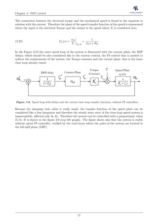
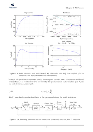
25. Chapter 3. FOC control
Gc (s) =
Kps + Ki
s
= Kp 1 +
1
Ti · s
(3.25)
The proportional gain of the PI controller is tuned until it becomes fast enough to fulfill the
requirements and then the integral is adjusted until a phase margin of 40o - 60o degrees is reached (no
disturbance) [15]. The bode plot with the gain margin is show in the figure 3.9.
Gc (s) =
0.3s + 3.2
s
(3.26)
The response of system with the tuned parameters is shown in figure 3.9 (bottom left graph).
0 0.1 0.2 0.3 0.4 0.5 0.6 0.7 0.8 0.9 1
0
0.2
0.4
0.6
0.8
1
1.2
Time [s] (seconds)
Amplitud[−]
Current inner loop
Speed outer loop
Figure 3.11. Current and speed close loop unit step response.
Finally the steps response of both, inner current close loop and outer speed close loop, are shown
together in the same graph 3.11, with the characteristics that archive the requirements for the FOC.
Characteristics of the outer speed close loop step response:
• Rise Time: 0.0682 [s]
• Settling Time: 0.5106 [s]
• Overshoot: 24.4254 %
Characteristics of the inner current close loop step response:
• Rise Time: 0.0020 [s]
• Settling Time: 0.0035 [s]
19

26. Chapter 3. FOC control
3.3.4 Anti windup
When the control of the current speed was designed, the limits of the system were ignored, however,
in reality there are limits. The voltage that is controlled by the inverter is fixed by the DC-link which
produces a limit in the current.
When high values of speed and torque are commanded, the limits are exceeded. In order to not exceed
these limits, the system is provided by a saturation block. The problem is that although this limit
is regulated by the saturation block, the machine will remain at the maximum limit, as shown in the
figure 3.13, for a long time due to the demands of the system. This reduces the time which the output
is at the saturation limit, reducing the damage to the machine and increasing its reliability [6].
In order to solve this problem an anti windup is introduced, so the limits will be respected and the
maximum limit will not remain for a long time and the response will be better as seen in the figure
3.13.
Figure 3.12 shows the PI controller structure with anti windup scheme [9].
pK
iK 1/ s
e
awK
u
Figure 3.12. PI controller structure with anti windup scheme [6].
It introduces a gain Kaw that increase the integral gain. Knowing that increasing the integral gain
will cause the overshoot on the close speed loop to decrease, Kaw is chosen as Kaw = 5 · Ki in each
control loop.
20

27. Chapter 3. FOC control
Figure 3.13. Current (top) and speed (bottom) response using anti windup [6].
As can be seen in the figure 3.13, where a step of 1000 RPM was performed, the response is better
when Kaw = 5 · Ki.
3.3.5 Voltage drops
Voltage drops can occur in the system due to:
1. Dead time in the inverter.
2. The internal connection in the inverter, the resistance of the cables and the on resistant transistors.
It is known that the time value for the death time is constant. When the inverter commands a small
value of the current, the desire duty cycle for the voltage should be small, and the percentage of
the dead time, in relation to the duty cycle time, is big. In the case that is studied in this report,
medium and high speed, the drop voltage produced by the dead time is neglected because the current
commanded is large enough.
The voltage drop of approximately 9 volts which appears in the dSPACE system [6] is accounted for
in the simulation model by adding the voltage drop.
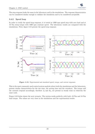
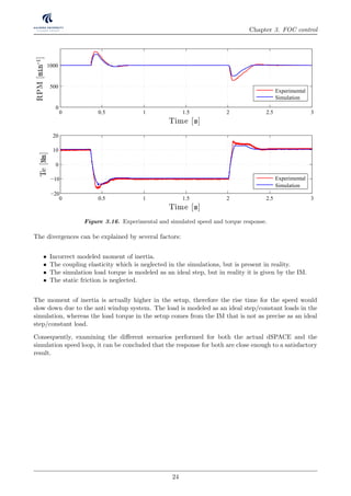
3.4 Simulation and Experimental results
In this section, the experimental results: current response and speed response, are presented. The
simulations made with Simulink should result in the same behavior as those observed in the laboratory.
The Control is implemented in the laboratory using dSPACE.
21

28. Chapter 3. FOC control
Table 3.1. Parameters used for simulation- and experimental verification.
System Description Parameter Value Unit
Current control
q-axis proportional gain kqp 2.5 [-]
q-axis integral gain kqi 135 [-]
d-axis proportional gain kdp 2.5 [-]
d-axis integral gain kdi 135 [-]
Voltage limit vlim 85 [V]
Speed control
Proportional gain kωp 0.3 [-]
Integral gain kωi 3.2 [-]
Current limit alim 20 [A]
Anti windup
Current integral gain kωaw 675 [-]
Speed integral gain kcaw 17.5 [-]
The table 3.1, shows the parameters obtained in the simulation which are implemented in the
laboratory in order to compare the results.
3.4.1 Current loop
The rotor is locked at zero degrees in the laboratory to observe the current loop step response. The
same is done in the simulations where the voltage drop is considered.
Figure 3.14. Experimental and simulated q-axis current loop step response (top) and d-axis current loop
step response(bottom) after including in the model the dead time and internal inverter voltage
drops.
Applying 10 amperes in the laboratory and in the simulation, the response is plotted in the same
graph for the d-axis and q-axis and shown in Figure 3.14 where the voltage drop is considered.
22

29. Chapter 3. FOC control
The step response looks the same in the laboratory and in the simulations. The response characteristics
can be considered similar enough to validate the simulation and to be considered acceptable.
3.4.2 Speed loop
In order to verify the speed loop response, it is tested at 1000 rpm speed step with zero load and at
10 Nm steep torque with 1000 rpm constant speed. The laboratory results are compared with the
simulations. First, figure 3.15 present the speed step response.
Figure 3.15. Experimental and simulated speed, torque, and current responses.
This is the most commonly used control system analysis where both the simulations and the laboratory,
present similar characteristics for the rise time, the setting time and the overshoot. The torque and
the currents respond accordingly, therefore J0 and Bm are present in steady state in relatively the
same scale.
Figure 3.16 below shows the next scenario. The system works perfectly with both -10 Nm and 10 Nm
load torque. The values are very close in the simulations and the experimental results.
23

30. Chapter 3. FOC control
Figure 3.16. Experimental and simulated speed and torque response.
The divergences can be explained by several factors:
• Incorrect modeled moment of inertia.
• The coupling elasticity which is neglected in the simulations, but is present in reality.
• The simulation load torque is modeled as an ideal step, but in reality it is given by the IM.
• The static friction is neglected.
The moment of inertia is actually higher in the setup, therefore the rise time for the speed would
slow down due to the anti windup system. The load is modeled as an ideal step/constant loads in the
simulation, whereas the load torque in the setup comes from the IM that is not as precise as an ideal
step/constant load.
Consequently, examining the different scenarios performed for both the actual dSPACE and the
simulation speed loop, it can be concluded that the response for both are close enough to a satisfactory
result.
24

31. Chapter 4
Sensorless Control
4.1 Introduction
The method FOC, presented in this project uses the speed and the position of the rotor to control the
PMSM. This can be achieved easily using a sensor. The disadvantages in terms of reliability, machine
size, noise interference and cost can be eliminated by removing the sensor and using a sensorless
control.
A general sensorless classification for a PMSM is presented in this chapter where it can be divided in
three strategies [12]:
• Model based estimators.
– Nonadaptive Methods.
– Adaptive Methods.
• Saliency Signal injection.
• Artificial Intelligence.
Model based estimators, Nonadaptive Methods: These methods use measured parameters of
the PMSM as fundamental machine equations to estimate the position. They can be divided into four
categories:
• Techniques using the measured DC-Link [16].
• Estimators using monitored stator voltages, or currents.
• Flux based position estimators.
• Position estimators based on back-EMF.
Model based estimators, Adaptive Methods: These are divided into four categories:
• Estimator based on Model Reference Adaptive System (MRAS).
• Observer-based estimators.
• Kalman estimator.
• Estimator which use the minimum error square.
Signal injection: After injecting voltage or current into the motor, the position and the speed can
be determined by processing the results. This method is divided in two categories:
• High frequency: The injection signal is large enough to neglect the resistance of the motor, and
the current depends only on the inductance.
• Low frequency: This method is based on the mechanical vibration of the rotor using low
frequency (few Hz).
25

32. Chapter 4. Sensorless Control
Artificial Intelligence
This describes neural network, fuzzy logic based systems and fuzzy neural networks [16].
This project is focused on an estimation of the speed and the position for medium and high speed using
the Back-EMF based sensorless algorithm which is mature enough and has already been combined
with vector control strategy in industrial applications. [20]. Therefore Back-EMF is selected to be
implemented to estimate the position of the shaft. The stator flux linkage vector can be estimated
to determine the rotor position angle using αβ stationary reference frames, and then integrated into
the equation, which can cause a drift. This problem can be avoided in different ways creating a sub-
classification to the Back-EMF method. This is presented and studied in detail in the next section.
4.2 Position estimation
In this section, the method Back-EMF for a surface permanent magnet mounted position estimation,
is introduced. This control algorithm is based on the estimation of the position using stator flux
linkage space vector in stationary αβ-reference frames. The dynamics of the motor can be obtained
by using the current and the voltage space vectors.
The mathematical structure of the estimation guarantees a high degree of robustness against parameter
variation [4] and simplicity [19].
The voltage equations are represented in stationary αβ-reference frames assuming that the inductances
are equal since the PMSM is surface mounted [19].
vα
vβ
=
Rs 0
0 Rs
·
iα
iβ
+
d
dt
λα
λβ
Where the stationary αβ flux linkage can be expressed through the rotor position:
λα
λβ
=
Lq 0
0 Lq
·
iα
iβ
+
cos θ
senθ
· λpm
So, from the above equations the position of the rotor can be estimated.
θ = tan−1 λβ − Lq · iβ
λα − Lq · iα
[rad/s](4.1)
The total flux linkage in stationary αβ-reference frames (λαβ) is now obtained by the equations 4.2
and 4.3:
λα = (vα − Rs · iα)dt [Wb](4.2)
λβ = (vβ − Rs · iβ)dt [Wb](4.3)
Where iαβ is the current obtained from the LEM modules, vαβ is obtained from the reference voltages
given by the current controllers, Rs is the stator phase resistance, θ is the rotor angular position in
26

33. Chapter 4. Sensorless Control
electrical radians, λpm is the peak value of the rotor PM flux linkage and Lq is the d-axis inductance.
Formediumtohighspeedrange,changes to the resistancesand inductances because of thethermaleffects,
can be neglected [10]
The problems that appear in this method, listed below, must be considered.
• Inaccurate measurements of inductance and resistance cause an error in the voltage that will
cause a drift after the integration.
• A small drift in the current will cause increasing error after integration [10].
These problems can be eliminated by means of a compensating function [4]. In the following, the
three different methods, Compensation block, Rasmussen and Rasmussen PI, will be introduced.
4.2.1 Compensation block
The voltage equation in stationary αβ-reference frames is show in the next equation 4.42:
vαβ = Rs · iαβ +
dλαβ
dt
[V](4.4)
In this equation, the voltage, is calculated by measuring the current and the parameters of the machine,
which are considered constants and accurate. Because this is not the reality, the margin of error can
be compensated by introducing a voltage compensation vcomp and the equation then becomes:
vαβ = Rs · iαβ +
dλαβ
dt
− vcomp [V](4.5)
vcomp compensates errors in the λdq estimation, such as inverter nonlinearity, dead time, integration
offset and resistance variance [7].
vcomp is calculated to be a constant value where the flux linkage in stationary αβ-reference frames,
calculated in different ways 4.7, 4.8, are compared and multiplied by a PI controlled 4.43, [10].
vcomp =
Kpcomp · s + Kicomp
s
· ¯λαβ − ¯λθ
αβ [V](4.6)
¯λαβ = (vαβ − Rs · iαβ)dt [Wb](4.7)
¯λθ
αβ = iθ
d · Ld + λpm + j · iθ
q · Lq · ej θ
[Wb](4.8)
Where ¯λθ
αβ is the flux linkage in stationary αβ-reference frames obtained using the position estimated
θ which can be calculated since the values of Ld, Lq, id, iq, and λpm are known and Kpcomp and Kicomp
are parameters that can be modified according to the needs of the system.
27

34. Chapter 4. Sensorless Control
The drawback of the integral parameter in the PI controller is that the initial response is very slow,
and the controller does not start to be effective until a certain amount of time has elapsed. Instead it
cancels the remaining error, which could be present with a proportional controller.
1
1 q sτ+
qsi*r
qsi1
1 dT s+ ∑
p iK s K
s
+ mω
tK
eT
+ − 1
m mB J s+
+ −
1c j
e θ
)
arg
mod
+
+
qL iαβ⋅ pmλ
offu
)
− +
θ
)
dqλ
+
j
e θ−
)
+
+
su R iαβ αβ− ⋅
qL iαβ⋅
compu
)
−
αβλ dqλ
iαβ
−
pmλ
arg
θ
)
dqLdqi θ
)
dq
θ
λ
)
θ
αβλ
)+
+
+
su R iαβ αβ− ⋅ αβλ dqλ
j
e θ
)
Figure 4.1. Diagram of the Back-EMF Compensation block method.
The diagram of the position estimation using the Compensation block method is show in figure 4.1.
4.2.2 Rasmussen
The Rasmussen Estimator method is presented in this section which estimates the rotor position using
the parameters of the machine and eliminates the drift using dq-reference frame flux linkage. When
λdq is estimated, to estimate the position, the voltage equation contains an offset produced because
of the measurements. It is introduced and modeled as ˆuoff . Therefore a new equation 4.9 for the flux
λdq become.
dλαβ
dt
= us − Rsis + ˆuoff [V](4.9)
λdq = λpm · ejˆθ
[Wb](4.10)
λαβ = Lq · iαβ + λdq [Wb](4.11)
Where ˆuoff is designed to lead to the flux estimate with constant amplitude λdq [5].
ˆuoff = C1 λpm − λdq ejˆθ
[V](4.12)
28

35. Chapter 4. Sensorless Control
The figure 4.2 shows the structure of the estimation position reproduced through the mathematical
equations using the Rasmussen method.
+ −
1c j
e θ
)
arg
mod
+
+
qL iαβ⋅ pmλ
offu
)
− +
θ
)
dqλ
+
+
+
su R iαβ αβ− ⋅
qL iαβ⋅
−
αβλ dqλ
arg
su R iαβ αβ− ⋅ αβλ dqλ
Figure 4.2. Diagram of the Back-EMF Rasmussen method.
The Rasmussen method is defined with a steady state error that depends on the parameters C1, on
the velocity measured in radians per second, and on δM defined in equation 4.13. δM turn depends
on λpm and λM [5].
δM =
λpm − λM
λM
[-](4.13)
λM = ¯λαβ − Lq ·¯iαβ [Wb](4.14)
¯θras = −
C1
ω
· δM [rad](4.15)
This shall be taken into account when control is designed since the higher value of C1 higher error
and a low value will result in pure damping and low bias [5]. It can be observed in figure 4.14.
29

36. Chapter 4. Sensorless Control
4.2.3 Rasmussen PI
A PI controller is introduced to the Rasmussen method. The constant C1 is substituted in order to
study the new response. So a new offset is defined in the next equation 4.16, called ˆuoffPI.
uoffPI =
Kpras · s + Kiras
s
· λpm − λαβ · ej θ
[V](4.16)
Therefore the new structure for the Rasmussen PI method becomes:
+ −
j
e θ
)
arg
mod
+
+
qL iαβ⋅ pmλ
offu
)
− +
θ
)
dqλsu R iαβ αβ− ⋅ αβλ dqλ
Figure 4.3. Diagram of the Back-EMF Rasmussen PI method.
30

37. Chapter 4. Sensorless Control
4.2.4 Comparison methods
Figure 4.4 shows the flux linkage in stationary αβ-reference frames in order to demonstrate that the
error produced by the drift has been removed. This is the main objective, and it is achieved for the
three methods. The comparison is made using the following parameters for the different methods:
• Compensation method Kicomp = 20 Kpcomp = 100
• Rasmussen PI method Kiras = 20 Kpras = 100
• Rasmussen method C1 = 100
These parameters are chosen looking for the most logical comparison while operating the PMSM at
1000 rpm speed with no load.
-1 -0.8 -0.6 -0.4 -0.2 0 0.2 0.4 0.6 0.8 1
-0.2
0
0.2
.ux linkage - [Wb]
.uxlinkage,[Wb]
λαβ
Compensation block
-1 -0.8 -0.6 -0.4 -0.2 0 0.2 0.4 0.6 0.8 1
-0.2
0
0.2
.ux linkage - [Wb]
.uxlinkage,[Wb]
λαβ
Rasmussen
-1 -0.8 -0.6 -0.4 -0.2 0 0.2 0.4 0.6 0.8 1
-0.2
0
0.2
.ux linkage - [Wb]
.uxlinkage,[Wb]
λαβ
Rasmussen PI
Figure 4.4. Simulation of the αβ flux linkage obtain by the different methods
Between Rasmussen and Rasmussen PI method, the Rasmussen method with proportional control C1
is the most appropriate choice for the control of the position estimation. Considering the permanent
magnet flux linkage λpm as the input and the flux linkage in dq reference frames λdq as the output,
the error is the difference between both. Considering this assumption, the close loop transfer function
is considered to be a first order system. Therefore, it is clear that λdq and λpm should have the same
value. Since it can be considered as a first order system, the disturbances are neglected. This first
order system has a negative pole on the real axis which makes it stable, as can be seen in Figure 4.5.
By adding a PI controller, besides the proportional parameter, an integral parameter is also added.
Using the same assumption as before, where λpm is the input and λdq is the output, Rasmussen PI
method results in a second order system for the close loop transfer function with two negative complex
31

38. Chapter 4. Sensorless Control
conjugates poles on the real axis. This can make the response of the system critically stable, as seen
in Figure4.5. Therefore the Rasmussen method is considered the best option.
0 0.05 0.1 0.15 0.2 0.25 0.3 0.35 0.4 0.45 0.5
-0.1
-0.05
0
0.05
0.1
Time [s]
Error[Wb]
Rasmussen PI
0 0.05 0.1 0.15 0.2 0.25 0.3 0.35 0.4 0.45 0.5
-0.1
-0.05
0
0.05
0.1
Time [s]
Error[Wb]
Rasmussen
Figure 4.5. Simulation data of the difference between |λdq| and the magnitude of λpm
Upon concluding that Rasmussen method is better than Rasmussen PI, the methods Compensation
block and Rasmussen are compared.
32

39. Chapter 4. Sensorless Control
-1 -0.8 -0.6 -0.4 -0.2 0 0.2 0.4 0.6 0.8 1
-0.2
0
0.2
.ux linkage - [Wb]
.uxlinkage,[Wb]
λαβ
Compensation block
-1 -0.8 -0.6 -0.4 -0.2 0 0.2 0.4 0.6 0.8 1
-0.2
0
0.2
.ux linkage - [Wb]
.uxlinkage,[Wb]
λαβ
Rasmussen
0 0.1 0.2 0.3 0.4 0.5 0.6 0.7 0.8 0.9 1
0
2
4
6
Time [s]
Position[rad]
θ Compensation block
θ Rasmussen
Figure 4.6. Simulation data of the αβ flux linkage and the position estimated obtain by the Compensation
block and Rasmussen methods.
Both Compensation block and Rasmussen method achieve good performances concluded with similar
response characteristics in steady state and during the dynamics.
Rasmussen is the preferred method because of the simplicity in the control since there is only one
parameter to control. Furthermore, Rasmussen method is the most recently developed method and
therefore has not been researched extensively.
33

40. Chapter 4. Sensorless Control
4.3 Inductance compensation
It is interesting to see from the equation 4.1, where the position is estimated, that Ld will not affect
the rotor position. In medium to high speed range the uncertainties about the stator resistance
variation due to thermal effect and inverter nonlinearities causing voltage estimation error can be
safely neglected. Therefore it is considered Lq inductance as the only and most important parameter
that will affect the estimated position error [11].
The inductance obtained from the machine is usually measured in an unsaturated region, and the
parameters Ld and Lq are considered as constant values which are not reliable. The inductance value
will decrease when the core of the machine is saturated, which occurs when the machine requires a
high current.
Since Lq is considered constant, an error will appear when the current increases causing the inductance
Lq to change.
When the core is saturated, no more magnetic flux can flow through the saturated section and therefore
the flux can be determined as a constant value. The flux will increase when the current increases, but
after saturation is reached, the change in the flux is negligible.
The flux linkage depends on B and S, where B is the magnetic field and S is the section of the material
that the flux flows through. The section is a constant value and depends on the construction of the
machine.
φ(B) = B · S [Wb](4.17)
B(H) depends on the Magnetic Field Strength (H), and the inductance depends on the flux φ(H).
L =
N · φ
i
[H](4.18)
In the saturated region, the flux does not change significantly, so increasing the current causes the
inductance to decrease.
Introducing a flux linkage term La ·¯iαβ in the stationary reference frame flux linkage the error can be
analyzed [11]. Where La an arbitrary constant inductance.
¯λαβ = La ·¯iαβ + (La − Lq) ·¯iαβ + (λpm + (Ld − Lq) · id) · ejθ
[Wb](4.19)
The term ¯iαβ is is replaced by ¯idq · ejθ and then the equation becomes
¯λαβ = La ·¯iαβ + ¯λeq · ejθ
[Wb](4.20)
where ¯λeq represent a special flux linkage vector.
¯λeq = λpm + (Ld(id, iq) − La) · id + j · (Lq(id, iq) − La) · iq [Wb](4.21)
34

41. Chapter 4. Sensorless Control
θ = ∠(¯λαβ − La ·¯iαβ) = ∠¯λeq + θ [rad](4.22)
The position error due to inductance variation is show in the equation 4.23.
θerr = ∠¯λeq = tan−1 (Lq(id, iq) − La) · iq
λpm + (Ld(id, iq) − La) · id
[rad](4.23)
Figure 4.7 shows the position error, according to the equation 4.23, the real and the estimated rotor
position.
errθ
θ
θ
)
( ( , ) )q d q a qL i i L i− ⋅
( ( , ) )pm d d q a dL i i L iλ + − ⋅
d axis−q axis−
a axis−
O
−
Figure 4.7. Vector position error produced by the inductance variation [11].
As seen from Figure 4.8, when La is considered as the unsaturated inductance value, an error will
appear when the current increases, causing the inductance Lq to change because the machine is in the
saturated region.
unsaturated
region
0
errθ
)
qi
Unsaturated inductance value
Unsaturated inductance value
aL =
aL <
Figure 4.8. Position error produced by artificial La [11].
The error can be reduced by 50%, by calculating the appropriate La < unsaturated inductance value,
using equation 4.23.
35

42. Chapter 4. Sensorless Control
4.3.1 Experimental study of the position error
In this section the rotor position error is measured by applying torque in order to experimentally
validate and verify the theory. At steady state the motor is running at 500 rpm and a load change is
introduced by the IM. It can be observed from the Figures 4.9, 4.10,4.11 that increasing the load will
cause the error to incrementally increase.
1 1.02 1.04 1.06 1.08 1.1 1.12 1.14
0
2
4
6
Time [s]
Position[rad]
θ Enconder
θ Sensorless
1 1.02 1.04 1.06 1.08 1.1 1.12 1.14
−0.5
0
0.5
Time [s]
Error[rad]
θ Error
−1 −0.8 −0.6 −0.4 −0.2 0 0.2 0.4 0.6 0.8 1
−0.2
−0.1
0
0.1
0.2
flux linkage [β]
fluxlinkage[α]
λ
α β
Figure 4.9. Laboratory position error and αβ flux linkage, at 5.5 Nm load condition (iq = 7.5 A).
The error produced in the Figure 4.9 does not increase excessively. This can be explained due to the
fact that the core does not reach the saturation region when the load is Torque = 5.5 Nm and the
current iq = 7.5 A.
In contrast, the Figures 4.10 and 4.11 show an increased error, indicating that the iron core is in the
saturation region.
Knowing the unsaturated inductance value La = 0.0022 H and the position error ¯θerr = −0.075 rad
when the current is at the maximum iq = 26.5 A, the new value of Lq(id, iq) is calculated. The error
is reduced by 50% just by applying the above equation 4.23. The new value of the inductance is
Lanew = 0.002 H. Considering Lanew = Lq, this is applied in equation 4.1 of the estimated position.
¯θerr = tan−1 (Lq(id, iq) − La) · iq
λpm + (Ld(id, iq) − La) · id
[rad](4.24)
Lq(id, iq) = 0.00185 [H](4.25)
Lanew =
La − Lq(id, iq)
2
+ Lq(id, iq) ≈ 0.002 [H](4.26)
36

43. Chapter 4. Sensorless Control
1 1.02 1.04 1.06 1.08 1.1 1.12 1.14
0
2
4
6
Time [s]
Position[rad]
θ Enconder
θ Sensorless
1 1.02 1.04 1.06 1.08 1.1 1.12 1.14
−0.5
0
0.5
Time [s]
Error[rad]
θ Error
−1 −0.8 −0.6 −0.4 −0.2 0 0.2 0.4 0.6 0.8 1
−0.2
−0.1
0
0.1
0.2
flux linkage [β]
fluxlinkage[α]
λ
α β
Figure 4.10. Laboratory position error and αβ flux linkage, at 12 Nm load condition (iq = 16.3).
1 1.02 1.04 1.06 1.08 1.1 1.12 1.14
0
2
4
6
Time [s]
Position[rad]
θ Enconder
θ Sensorless
1 1.02 1.04 1.06 1.08 1.1 1.12 1.14
−0.5
0
0.5
Time [s]
Error[rad]
θ Error
−1 −0.8 −0.6 −0.4 −0.2 0 0.2 0.4 0.6 0.8 1
−0.2
−0.1
0
0.1
0.2
flux linkage [β]
fluxlinkage[α]
λ α β
Figure 4.11. Laboratory position error and αβ flux linkage, at 19.5 Nm load condition (iq = 26.7).
Therefore the theory is verified experimentally, where the error is explained by the equations 4.23
37

44. Chapter 4. Sensorless Control
4.4 Speed estimator
In this report a Phase-Locked Loop (PLL) is designed to obtain the estimated speed. The block
diagram of the PLL is shown in Figure 4.12. It introduces a PI controller in the open loop that
contains two important parameters Kep and Kei. The integral of the speed is the position. Therefore
after the integral in the closed loop the position can be retrieved.
mω
j
e θ
)
+
offu
)
θ
)
−
*
θ
) ω
)
PLLθ
)
Figure 4.12. Phase lock loop (PLL) diagram.
Based on Figure 4.12 above, a new value of the position estimation θPLL is obtained.
θPLL
=
1 · Kep · S + Kip
s2
· θ − θPLL
[rad](4.27)
The transfer function in the Laplace domain is obtained in order to design the parameters Kep and
Kei, where θPLL
r is the output and θr the input.
θPLL
θ
=
Kep · s + Kip
s2 + Kep · s + Kip
[-](4.28)
Where θPLL
r is equal to θr in steady state. Therefore the error is zero.
38

45. Chapter 4. Sensorless Control
4.5 Control design
The control structure for sensorless control is shown in Figure 4.13.
ω
LELEM
Enconderdataforspeedmeasurement
CurrentandVoltagemeasurement
ic refV −
VSI
Inverter
SVM
r
q q rL i ω
r
d d r r PML i ω ω λ+
abc
PMSM
Position
estimation
0
*r
dv
*r
qi
ci bi
Position
transducer
Speed
controller
Current
controllers
V
DCV
rθ
)
*r
qv
*r
di
mω∗
mω −
+ +
−
+
−
+
−
+ +
vα
vβ
dq
abc
αβ
uαβ
iαβ
Position
estimation
Speed
estimation
rθ
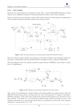
Figure 4.13. General sensorless scheme using Field Oriented Control.
The position estimation takes the values of the current and voltage in stationary αβ-reference frames
for the back-EMF Rasmussen method and the speed estimation takes the position for the PLL.
4.5.1 Position estimator
The Back-EMF Rasmussen based position estimation algorithm has a constant parameter that can be
controlled. The parameter is called C1 which is multiplied by the difference between |λdq| and λpm.
It is introduced in equation 4.16 where the offset is altered to eliminate the drift. C1 the response
will be faster in the dynamics ”The higher C1 the higher speeds that could be reached and vice versa
for lower speeds”[13]. This make sense because, as it is mentioned in [5] ”C1 is a balance between
damping and bias, meaning that a low value will result in pure damping and low bias and visa versa”.
|λdq| response, which depends on C1, is also investigated. This response is faster with a higher value
of C1 and vice versa. The time response also depends on the error between λdq and λpm, being faster
the higher the error, so it is continuously adapted to demand.
C1 is determined in terms of λdq , speed and position response running the machine from the worst-
case scenario which is the lower speed when C1=50 and the speed is 200 rpm.
39

46. Chapter 4. Sensorless Control
4 6 8 10 12 14
0.1215
0.122
0.1225
Time [s]
Fluxlinkage[Wb]
|λdq
| response
0.4 0.5 0.6 0.7 0.8 0.9 1
0
2
4
6
Time [s]
Position[rad]
θ Enconder
θ Sensorless
4 6 8 10 12 14
200
400
600
800
1000
1200
Time [s]
Speed[r.p.m]
n Enconder
n Sensorless
Figure 4.14. Response of the λdq , Speed and the position estimated. When C1 = 50 and the speed PI
controllers are Kiw=0.1 and Kwp=0.05
From Figure 4.14 it can be seen that for higher speeds, with the same value of C1, difference between
λpm and λdq decreases knowing λdq = 0.12258 Wb. Additionally the figure shows that the response is
fast enough with values of C1 = 50.
Thus, according to the equations 4.13 and 4.15, the ratio C1 divided by ω is set as a constant value
so C1 will be capable of different speeds values.
Being able to increase the C1 value in the equation 4.15 for higher speeds, improves the response and
maintains a constant error value. The ratio is assigned to be C1 / ω = 0.6.
40

47. Chapter 4. Sensorless Control
4.5.2 Speed estimator
In this section, the parameters of the PLL are tuned in order to get the required response.
The PLL transfer function can be rewritten as a standard second order transfer function 4.29.
θPLL
r
θr
=
Kep · S + Kip
S2 + Kep · S + Kip
=
ω2
n
S2 + 2 · ξ · ωn + ω2
n
[-](4.29)
The existing relation between both transfer functions allows the PIP LL controllers parameters, Kei
and Kep, to be calculated when [2] the desired bandwidth and damping ratio are known.
Kep = Bω 2.2 · ξ − 0.668 · ξ2
[-](4.30)
Kei = B2
ω (1.1 − 0.334 · ξ)2
[-](4.31)
From the relation in the equation 4.32, ωr can be calculated which is the input frequency of the PLL
ω =
n · 2 · π · pp
60
[rad/s](4.32)
Where the bandwidth can be related to the input frequency, as is shown in the following equation,
fulfilling the condition 4.33.
0 ω Bw [rad/s](4.33)
So the equation 4.34 is assumed in order to tune the PIPLL parameters.
ω = Bw [rad/s](4.34)
Therefore from Bw the control parameters can been calculated:
Kep = Bw 2.2 · ξ − 0.668 · ξ2
[-](4.35)
Kei = Bw2
(1.1 − 0.334 · ξ)2
[-](4.36)
41

48. Chapter 4. Sensorless Control
0 0.05 0.1
0
0.5
1
1.5
2
Step Response
Time (seconds)
Amplitude
-50
0
50
Magnitude(dB)
System: G1
Frequency (rad/s): 355
Magnitude (dB): -3.59
10
1
10
2
10
3
10
4
-180
-90
0
Phase(deg)
Bode Diagram
Frequency (rad/s)
0 0.02 0.04 0.06 0.08 0.1
0
0.5
1
1.5
Step Response
Time (seconds)
Amplitude
10
1
10
2
10
3
-90
-45
0
Phase(deg)
Bode Diagram
Frequency (rad/s)
-20
0
20
Magnitude(dB)
System: G11
Frequency (rad/s): 210
Magnitude (dB): -2.84
Figure 4.15. Speed close loop unit step response and close loop bode diagram with old PI controllers (top
graphs) and new PI controllers (bottom graphs) showing the bandwidth
For different speed values, the corresponding frequency determines the bandwidth and consequently
the final values for Kep and Kei where the damping ratio is set as ξ = 0.2. In the case studied when
n=500 rpm, the condition 4.33 is fulfilled, where ω = 209.43 rad/s.
ω =
n · 2 · π · pp
60
=
500 · 2 · π · 4
60
= 209.43 [rad/s](4.37)
Figure 4.15 shows the bandwidth when applying the above assumption to the equations 4.35 and 4.36
where the value is too large (Bw=355 rad/s). It can be a problem when higher frequencies than ωr
appear in the rotor position.
In order to eliminate the undesired frequencies, we use the frequency in Hz so ωr will decrease 2 · π
and then, the bandwidth becomes smaller. The equations 4.45 and 4.39 [17] are used increasing Kep
ten times. Bw = 215 rad/s is the new and more appropriate bandwidth for fulfilling the condition
4.33.
PIPLL = Kep 1 +
1
Ti · s
[-](4.38)
42

49. Chapter 4. Sensorless Control
Kep =
9.2
ts
[-](4.39)
4.5.3 Sensorless
When the system operates without an encoder, the speed loop parameters should be modified. A
delay is introduced, as a feedback in the system, by the position and speed estimation as it is shown
in Figure 4.16. In this way, the variation of the poles can make the system unstable. ω
CPG
r
qsi*r
qsi1
1 dT s+
DSP-delays Current Plant
mω∗ +
−
p iK s K
s
+
Speed
PI-controller
Speed Plant
q-axis
mω
tK
Torque
Constant
eT
lT
+ −
s
nt
mω
1
m mB J s+
1
s qR L s+
r
qsi*r
qsi +
−
1
1 dT s+
p iK s K
s
+
PI-controller DSP-delay PMSM-Plant
j
e θ−
)
compu
)
iαβ
−
pmλ
θ
)
dqLdqi θ
)
dq
θ
λ
)
θ
αβλ
)+
+
+
j
e θ
)
1
1 osτ+
Position and
speed
estimation uαβ
iαβ
Figure 4.16. speed close loop where the sensorless control is used as the feedback.
Where τ0 is defined as a time constant. The new close loop transfer function becomes:
Gcl(s) =
G(s)
1 + G(s) · H(s)
[-](4.40)
where:
H(s) =
1
1 + τ0
[-](4.41)
The higher value of τ0 is used for the control because it causes the worst case. By applying this
assumption, the bandwidth is calculated when the system is running at 200 rpm which can be obtained
from the bode plot. By applying a simplification, the second order closed loop PLL transfer function
is considered as a first order system.
H(s) =
1
1 + τ0
[-](4.42)
where τ0 is determined based on the sensorless bandwidth using the equation 4.43.
Bw =
1
τ0
[rad/s](4.43)
The figure 4.17 below shows the bode diagram in close and open loop, and the root locus, using the
new control values Ki and Kp for the PI speed loop controller where PI controllers are adjusted until
a phase margin of 40o - 60o is reached (no disturbance)[14].
43

50. Chapter 4. Sensorless Control
10
0
10
2
10
4
-360
-180
0
Frequency (rad/s)
Phase(deg)
-200
-100
0
100
Bode Editor for Closed Loop 1(CL1)
Magnitude(dB)
10
0
10
5
-450
-360
-270
-180
-90
P.M.: 56.3 deg
Freq: 3.03 rad/s
Frequency (rad/s)
Phase(deg)
-250
-200
-150
-100
-50
0
50
100
G.M.: 51.3 dB
Freq: 267 rad/s
Stable loop
Open-Loop Bode Editor for Open Loop 1(OL1)
Magnitude(dB)
-10000 -5000 0 5000
-1
-0.5
0
0.5
1
x 10
4 Root Locus Editor for Open Loop 1(OL1)
Real Axis
ImagAxis
Figure 4.17. Open and close loop Bode diagram and root locus for speed controller.
The control values for the estimation of speed and position are selected as shown in Table 4.1. Once
the correct estimate has been made for speed and position the FOC is updated. The parameters
shown will be implemented for both the simulation and in the laboratory.
Table 4.1. Parameters used for sensorless control.
System Description Parameter Value Unit
Current control
q-axis proportional gain kqp 2.5 [-]
q-axis integral gain kqi 135 [-]
d-axis proportional gain kdp 2.5 [-]
d-axis integral gain kdi 135 [-]
Voltage limit vlim 85 [V]
Speed control
Proportional gain kωp 0.05 [-]
Integral gain kωi 0.1 [-]
Current limit alim 20 [A]
Anti windup
Current integral gain kωaw 675 [-]
Speed integral gain kcaw 17.5 [-]
44

51. Chapter 4. Sensorless Control
4.5.4 Auto tuning
Based on the control design, the parameters of the PIPLL and the Back-EMF Rasmussen method
control can be modified in relation to the speed operation in order to get a better response.
Figure 4.18 shows the new schematic version of the control where the Auto-tunings are implemented
on the position and speed estimation based on the reference speed.
ω
LELEM
Enconderdataforspeedmeasurement
CurrentandVoltagemeasurement
ib refV −
ic refV −
VSI
Inverter
SVM
r
q q rL i ω
r
d d r r PML i ω ω λ+
abc
PMSM
Position
estimation
0
*r
dv
*r
qi
ci bi
Position
transducer
Speed
controller
Current
controllers
V
DCV
rθ
)
*r
qv
*r
di
mω∗
mω −
+ +
−
+
−
+
−
+ +
vα
vβ
dq
abc
αβ
uαβ
iαβ
Position
estimation
mω∗
Speed
estimation
rθ
ω∗
m
Figure 4.18. General sensorless auto-tuning scheme using Field Oriented Control.
when the reference speed is known, the frequency of the input variables in the sensorlees control are
also known, and therefore the PI controller should be changed in order to adapt the Bandwidth.
The block diagram 4.19 of the position estimation control system of PMSM by auto-tuning C1 shown
how it is implemented.
+ −
*
1 ( )mC ω j
e θ
)
arg
mod
+
+
qL iαβ⋅ pmλ
offu
)
− +
θ
)
dqλsu R iαβ αβ− ⋅ αβλ dqλ
mω∗
+
−
offu
)
*
( )ep mK ω
*
( )ei mK ω 1/ s
+
+
mω∗
mω∗
Figure 4.19. Diagram of the position estimation with auto-tuning.
The concept of the Rasmussen control includes auto-tuning making the response faster when the
difference between λdq and λpm increases and vice versa. The parameter C1 makes it even faster.
Therefore tuning C1 to the worst case, based on the control of the equation 4.15, the ratio C1/¯ω is
kept constant. This allows C1 to be increased for higher speeds without increasing the error. The
equation 4.46 shows the C1 Auto-tuning control where ω is considered to be the same as the reference
estimated ω∗ and the ratio C1/¯ω = 0.6.
45

52. Chapter 4. Sensorless Control
The block diagram 4.20 of the speed estimation control system of PMSM by auto tuning the PIPLL
parameters shows how it is implemented.
+ −
arg
mod
+
+
qL iαβ⋅ pmλ
− +
dqλsu R iαβ αβ− ⋅ αβλ dqλ
+
−
*
( )ep mK ω
*
( )ei mK ω
+
+
mω∗
θ
)
PLLθ
)
ˆ
mω∗
ω
Figure 4.20. Diagram of the speed estimation with auto-tuning .
Based on the control design, the parameters of the PIPLL must be auto tuned in relation to the speed
reference using the equations 4.44 and 4.45
Kep(ω∗
) =
ω∗
2 · π
· 2.2 · ξ − 0.668 · ξ2
· 10 [-](4.44)
Kei(ω∗
) =
ω∗
2 · π
2
· (1.1 − 0.334 · ξ)2
· 10 [-](4.45)
When the Auto-tuning is done, a problem appears if the machine has a reference speed of zero. At
zero speed, C1 is equal to zero, meaning that the Rasmussen method is not working, and therefore,
the drift will appear after the integral. This is solved by adding a constant value K1 as is shown in
the equation 4.46. The value K1 is assigned as K1 = 10.
C1(ω∗
) = 0.6 · ω∗
+ K1 [-](4.46)
As an example the values of the PIPLL controller and C1 are calculated using the Auto-tuning when
the reference speed n∗ = 500 rpm. The value of ω∗ = 209.43 rad/s is calculated using following
equation 4.47.
ω∗
=
n∗ · 2 · π · pp
60
[rad/s](4.47)
Knowing the reference speed ω∗ = 209 rad/s, the damping ratio ξ = 0.2 and the constant K1 = 10,
the parameters of the controllers can be calculated using equations 4.46, 4.45 and 4.44: C1(ω∗) = 310,
Kep(ω∗) = 137.8 and Kei(ω∗) = 1861.
46

53. Chapter 5
Sensorless Experimental results
In this chapter the laboratory results for the sensorless rotor field oriented control of PMSM are
presented by several setup scenarios. The position and the speed are measured by the encoder in
order to compare and verify the results obtained the by sensorless control algorithm, using the Auto-
tuning for both the position estimation and the speed estimation.
In each of the graphs below showing position error, errors above 0.5 are as a result of errors in the
measurements.
5.1 Speed steps with no load.
In this case, the sensorless control is tested with no load for both negative and positive speed values
which are applied incrementally in speed steps.
5.1.1 Decreasing and increasing steps at positive speed.
0 5 10 15 20 25 30
0
500
1000
Time [s]
Speed[r.p.m]
n Encoder
n Sensorless
0 5 10 15 20 25 30
−10
−5
0
5
Time [s]
Current[A]
iq
id
0 5 10 15 20 25 30
−10
0
10
Time [s]
Torque[Nm]
Torque PMSM
Torque IM
Figure 5.1. Experimental speed, torque, and current, in dq reference frames, responses.
47

54. Chapter 5. Sensorless Experimental results
1.3 1.35 1.4 1.45 1.5
0
2
4
6
Time [s]
Position[rad]
θ Enconder
θ Sensorless
1.3 1.35 1.4 1.45 1.5
−0.5
0
0.5
Time [s]
Error[rad]
θ Error
8 8.05 8.1 8.15 8.2
0
2
4
6
Time [s]
Position[rad]
θ Enconder
θ Sensorless
8 8.05 8.1 8.15 8.2
−0.5
0
0.5
Time [s]
Error[rad]
θ Error
12.1 12.12 12.14 12.16 12.18 12.2
0
2
4
6
Time [s]
Position[rad]
θ Enconder
θ Sensorless
16 16.1 16.2 16.3 16.4 16.5
−0.5
0
0.5
Time [s]
Error[rad]
θ Error
Figure 5.2. Experimental estimated angle response compared with the real angle response (right). Position
error of the estimated angle response (left).
In the graph from the figure 5.1, it can be seen how the speed is increasing from 300 rpm until 1200
rpm by steps of 200 rpm. A good response in both steady and dynamic states is noticeable. The graph
of the idq current takes the angle of the position estimation. The id current follows the zero reference,
while, on the other hand iq differs from zero in order to face the torque produced by Tload, Bm, J0
and Jm. When there are changes in speed due to inertia, peaks in the iq values appear. Finally, the
graph of the Torque is shown in order to verify that there is no load, and to demonstrate how this
affects the current.
Figure 5.2 shows the position estimation and the error for three different speeds. In these three cases,
the error is almost negligible. In the first case there is an oscillation that can be produced due to the
value of C1 which is auto tuned to be very low.
5.1.2 Decreasing and increasing steps at negative speeds.
The motor is tested now at a negative speed to verify that it has the same response. Figures 5.3 and
5.4 show that the behavior is almost the same for both.
Therefore it is verified that the response is appropriate for the position and speed estimation, and
correct operation of the auto tuning is seen when the sensorless control of the PMSM in running
without any load.
48

55. Chapter 5. Sensorless Experimental results
5 10 15 20 25 30 35 40
−1000
−500
0
Time [s]
Speed[r.p.m]
n Encoder
n Sensorless
5 10 15 20 25 30 35 40
−10
−5
0
5
Time [s]
Current[A]
iq
id
5 10 15 20 25 30 35 40
−10
0
10
Time [s]
Torque[Nm]
Torque PMSM
Torque IM
Figure 5.3. Experimental speed, torque, and current, in dq reference frames, responses.
Where figures 5.3 and 5.4 show that the behavior is almost the same for positive and negative values.
3.3 3.35 3.4 3.45 3.5 3.55
0
2
4
6
Time [s]
Position[rad]
θ Enconder
θ Sensorless
3.3 3.35 3.4 3.45 3.5 3.55
−0.5
0
0.5
Time [s]
Error[rad]
θ Error
12 12.05 12.1 12.15 12.2
0
2
4
6
Time [s]
Position[rad]
θ Enconder
θ Sensorless
12 12.05 12.1 12.15 12.2
−0.5
0
0.5
Time [s]
Error[rad]
θ Error
22.6 22.65 22.7 22.75 22.8
0
2
4
6
Time [s]
Position[rad]
θ Enconder
θ Sensorless
22.6 22.65 22.7 22.75 22.8
−0.5
0
0.5
Time [s]
Error[rad]
θ Error
Figure 5.4. Experimental estimated angle response compared with the real angle response (right). Position
error of the estimated angle response (left).
49

56. Chapter 5. Sensorless Experimental results
5.2 Speed steps with constant load torque.
In this case speed steps are applied with a constant 10 Nm torque as a load. After the torque is
commanded speed steps are applied increasing and decreasing the values of it.
0 5 10 15 20 25 30 35 40
0
500
1000
Time [s]
Speed[r.p.m]
n Encoder
n Sensorles
0 5 10 15 20 25 30 35 40
−10
0
10
20
Time [s]
Current[A]
iq
id
0 5 10 15 20 25 30 35 40
−10
0
10
Time [s]
Torque[Nm]
Torque PMSM
Torque IM
Figure 5.5. Experimental speed, torque, and current, in dq reference frames, responses.
Figure 5.5 shows how the speed responds properly for all speed ranges. In this case, in contrast to the
preceding case, when a load is applied the behavior of the estimated speed response is better. This
can be explained because of the higher current demand.
Figure 5.6 shows seen the currents abc stationary reference frames for different speeds, where the
response is correct.
The position estimation shows an error that is corrected for increasing speeds. If there is a difference
between λpm and λdq the error increases with lower speeds in accordance with the equations 4.15 and
4.13
This error is transformed by losses as it can be observed from figure 5.5 (current in dq reference frames
graph). These losses are shown by the torque having a higher value than the one that is applied by
the load.
50

57. Chapter 5. Sensorless Experimental results
0 0.02 0.04 0.06 0.08 0.1 0.12 0.14 0.16 0.18 0.2
−20
0
20
Time [s]
Current[A]
ia
ib
ic
8.5 8.52 8.54 8.56 8.58 8.6 8.62 8.64 8.66 8.68 8.7
−20
0
20
Time [s]
Current[A]
ia
ib
ic
16 16.02 16.04 16.06 16.08 16.1 16.12 16.14 16.16 16.18 16.2
−20
0
20
Time [s]
Current[A]
ia
ib
ic
Figure 5.6. Experimental currents in abc stationary reference frames.
2.7 2.72 2.74 2.76 2.78 2.8
0
2
4
6
Time [s]
Position[rad]
θ Enconder
θ Sensorless
2.7 2.72 2.74 2.76 2.78 2.8
−0.5
0
0.5
Time [s]
Error[rad]
θ Error
8 8.05 8.1 8.15 8.2
0
2
4
6
Time [s]
Position[rad]
θ Enconder
θ Sensorless
8 8.05 8.1 8.15 8.2
−0.5
0
0.5
Time [s]
Error[rad]
θ Error
12.1 12.12 12.14 12.16 12.18 12.2
0
2
4
6
Time [s]
Position[rad]
θ Enconder
θ Sensorless
16 16.1 16.2 16.3 16.4 16.5
−0.5
0
0.5
Time [s]
Error[rad]
θ Error
Figure 5.7. Experimental estimated angle response compared with the real angle response (right). Position
error of the estimated angle response (left).
51

58. Chapter 5. Sensorless Experimental results
5.3 Constant speed command with load torque steps.
In the final case the PMSM behavior with constant speed and applying torque steps is studied.
2 4 6 8 10 12 14 16 18 20
−10
0
10
Time [s]
Torque[Nm]
Torque PMSM
Torque IM
2 4 6 8 10 12 14 16 18 20
−10
0
10
20
Time [s]
Current[A]
2 4 6 8 10 12 14 16 18 20
600
800
1000
Time [s]
Speed[r.p.m]
n Enconder
n Sensorless
iq
id
Figure 5.8. Experimental speed, torque, and current, in dq reference frames, responses.
Figure 5.8 shows the idq current and torque responses. The value of the speed corresponds to the
frequency of the sinusoidal signal of the iabc currents shown in figure 5.9. The idq current value shows
the corresponding values of the current for different load values where the id current is kept constant
and equal to 0 and the iq current varies in function of the torque. That explains the correct position
estimation. In figure 5.10, the estimated and the real angle positions are measured for different load
values and for the variation interval of torque between 7 and 8 Nm in order to test the stationary and
the dynamic state response.
52

59. Chapter 5. Sensorless Experimental results
2.6 2.62 2.64 2.66 2.68 2.7 2.72 2.74 2.76 2.78
−5
0
5
Time [s]
Current[A]
ia
ib
ic
8.9 8.92 8.94 8.96 8.98 9 9.02 9.04 9.06 9.08 9.1
−10
0
10
Time [s]
Current[A]
ia
ib
ic
20.8 20.82 20.84 20.86 20.88 20.9 20.92 20.94 20.96 20.98 21
−20
0
20
Time [s]
Current[A]
ia
ib
ic
Figure 5.9. Experimental steady state currents in abc stationary reference frames.
2.7 2.72 2.74 2.76 2.78 2.8
0
2
4
6
Time [s]
Position[rad]
θ Enconder
θ Sensorless
2.7 2.72 2.74 2.76 2.78 2.8
−0.5
0
0.5
Time [s]
Error[rad]
θ Error
20.7 20.72 20.74 20.76 20.78 20.8
0
2
4
6
Time [s]
Position[rad]
θ Enconder
θ Sensorless
20.7 20.72 20.74 20.76 20.78 20.8
−0.5
0
0.5
Time [s]
Error[rad]
θ Error
12.1 12.12 12.14 12.16 12.18 12.2
0
2
4
6
Time [s]
Position[rad]
θ Enconder
θ Sensorless
12.1 12.12 12.14 12.16 12.18 12.2
−0.5
0
0.5
Time [s]
Error[rad]
θ Error
Figure 5.10. Experimental estimated angle response compared with the real angle response (right). Position
error of the estimated angle response (left).
53

61. Chapter 6
Conclusion
FOC is the procedure used to control the machine while the park‘s transformations are used to simplify
the control. The current PI controllers are tuned by applying Internal Model Control (IMC), and a
speed PI controller is tuned, considering the requirements of the system. BEMF contribution is
decoupled and the known dSPACE delays and drop voltage are considered in the simulations. An
anti-windup is introduced in order to prevent possible damage to the machine.
Sensorless control is used in order to eliminate the sensor which has advantages in terms of reliability,
machine size, noise and cost. Back-EMF is the method selected to be implemented to estimate the
position using the stationary αβ-reference frames where the integral in equation 4.1 that is used
to estimate the position, can cause a drift which occurs because of inaccurate measurements of the
parameters or because of a small drift in the current. This can be eliminated using different methods.
The methods Compensation block and Rasmussen are compared as they use different ways to solve the
problem produced by the drift. An integral gain is added in the Rasmussen (Rasmussen PI) method
in order to improve the response and eliminate the constant error, if present, but it causes a problem
in terms of stability as is explained in Chapter 4.
The Back-EMF Rasmussen is the selected method to estimate the position because of the simplicity
in the control and because it is the most recently developed method where the parameter C1 need to
be tuned in order to obtain an accurate response.
C1 can be controlled according to the speed, ”the higher C1, the higher speeds that could be reached
and vice versa for lower speeds”.
Phase-locked loop (PLL) is the method selected to be implemented to estimate the speed where the
PIPLL controller needs to be tuned. The PIPLL controller can be tuned according to the bandwidth.
Using 4.35 and 4.36, the theory demonstrates that the bandwidth is too large which causes a problem
when higher frequencies than ωr appear in the estimation of the rotor position. The undesired
frequencies are eliminated by dividing the Bandwidth by 2 · π and using the equations 4.45 and 4.39
to achieve a faster response, increasing Kep and Kei by a factor of ten. A new and more appropriate
bandwidth for fulfilling the condition of 4.33 is achieved.
The delay that appears in the feedback of the system from the estimated position and the speed should
be considered. The delay is considered at the worst case, that is when the machine is running at the
lower speed (n = 200 rpm). The new speed PI controller’s Kwi and Kwp are considered achieving the
requirements of the system for FOC.
A position error θerr can be caused when the core of the machine is saturated, which occurs when the
machine requires a high current. The theory is verified experimentally as is shown in Figures 4.9, 4.10
and 4.11 and the error is reduced successfully by 50% using equation 4.24 and 4.26.
The position error θras has to be considered since the Rasmussen method is used. Notice that the
error can be kept constant if the ratio C1/¯ω is kept constant.
The Auto-tuning for the position estimation is done, tuning C1 for the worst-case scenario study (n
= 200 rpm) and setting constant, the ratio C1 divided by ω considering ω = ω∗. Therefore C1 can be
tuned as a function of ω∗.
55

62. Chapter 6. Conclusion
The Auto-tuning for the speed estimation is done considering the bandwidth as a function of ω∗ using
equations 4.35, 4.36, 4.45 and 4.39.
Therefore, the Auto-tuning is implemented for both position and speed estimation. It consists of the
on-line control of the parameters C1 for the position estimation method, and Kep and Kip for the
speed estimation method, based on speed reference using the equation 4.46 for the auto-tuning of C1
and 4.44 and 4.45 for the Kep and Kip respectively.
In Chapter 5, results for the sensorless rotor Feld Oriented Control of PMSM are presented for several
setup scenarios, where the position and the speed are measured using the encoder in order to verify
the results obtained by the Auto-tuning sensorless control.
The results are accurate for a range of speeds from -1400rpm to -300rpm and from 300 rpm to 1400,
supporting a load of ± 10 Nm.
When no load is applied there is almost no error in the position and the speed estimation, but at low
speed a big oscillation appears. On the other hand, when load is applied no oscillations appear but
position error increases. Overall, the control operated correctly, achieving satisfactory results.
56

63. Chapter 7
CD Content
• Report(PDF)
• Simulink Model
• dSPACE Model
• System Data Tests
• References and literature
57

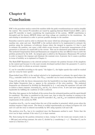
65. Bibliography
[1] Andres Lopez-Aranguren Oliver, Cesar Hernaez, E. B. N. J. M. (2013). Auto-tuning of high
performance vector controller for pmsm drive system.
[2] Chen, J.-L. C. T.-H. L. C.-L. (2009). Design and implementation of a novel high-performance
sensorless control system for interior permanent magnet synchronous motors.
[3] de Ciencias Basicas Universidad Iberoamericana, D. (2000). Control de modelo interno.
[4] Fabio Genduso, Rosario Miceli, M. I. C. R. and Galluzzo, G. R. (2000). Back emf
sensorless-control algorithm for high-dynamic performance pmsm.
[5] H. Rasmussen, P. . V. a. and Brsting, H. (2012). Sensorless field oriented control of a pm motor
including zero speed.
[6] Hernaez, C. (2014). Snsorless control of pmsm.
[7] Ion Boldea, Fellow, I. M. C. P. and Gheorghe-Daniel Andreescu, Senior Member, I. (2008).
Active flux concept for motion-sensorless unified ac drives.
[8] Javier Fernndez Martnez, T. P. S. (2011). Low speed open loop field oriented control for
permanent magnet machines.
[9] Jordi Espina, Toni Arias, J. B. C. (2006). Speed anti-windup pi strategies review for field
oriented control of permanent magnet synchronous machines.
[10] Kaiyuan Lu, A. (2014). Modern electrical machine and drive systems sensorless control of pm
machines.
[11] Kaiyuan Lu, Member, I. X. L. and Frede Blaabjerg, Fellow, I. (2008). Artificial inductance
concept to compensate nonlinear inductance effects in the back emf-based sensorless control
method for pmsm.
[12] O. Benjak, D. G. (2010). Review of position estimation methods for ipmsm drives without a
position sensor.
[13] Pedersen, A. R. (2012). Comparison of back-emf based methods for sensorless control of a
pmsm.
[14] Phillips, C. L. and Harbor, R. D. (2000). Feedback control systems. prentice hall.
[15] Phillips, C. L. and Harbor, R. D. (2011). Feedback control systems.
[16] P.S Frederiksen, J. Birk, F. (1994). Control and instrumentation for pm-machines.
[17] Remus Teodorescu, Marco Liserre, P. R. (2011). Grid converters for photovoltaic and wind
power systems.
[18] Wang, D. (2013). Introduction of synchronous reluctance machine.
[19] Zihui Wang, Student Member, I. K. L. and Frede Blaabjerg, Fellow, I. (2012). A simple startup
strategy based on current regulation for back-emf-based sensorless control of pmsm.
[20] Zihui Wang, Qinfen Lu, Y. Y. K. L. Y. F. (2000a). Investigation of pmsm back-emf using
sensorless control with parameter variations and measurement errors.
59

66. Chapter BIBLIOGRAPHY
[21] Zihui Wang, Kaiyuan Lu, Y. Y. Y. J. W. H. (2000b). Analysis of influence on back-emf based
sensorless control of pmsm due to parameter variations and measurement errors.
60

67. Appendix A
VSI modulation strategy
The two level three phase Voltage Source Inverter is controlled by using SVM. SVM is used in the
system due to the advantages such as it improves the DC-link utilization by 15.5% The Figure A.2
represent the phase voltage space vectors.
:;<
=><
?
;
@A
BA
CA
DA
EA
FA
GH:=
J;<
>;<
KLNOOPQ KR
STUVWXYZ[Z!#$%#'()*!+%),0
]^3_^ #*2`^ #2a*2#$#$*'#!#$3 -b#*2c #2a*2#$
$--!#*2*#-!4-*#$678-*90/#$2*-$-(#*5#$$'42#*
-2-d*#*22-$-*($-(-*$--*$#$$-50)*.-'/0e$-f$-$--*$
#$*0
ghi
j
k
lm
nm
om
pm
qm
rm
stug
v
ghi
j
k
lm
nm
om
pm
qm
rm
stug
v
ghi
j
k
lm
nm
om
pm
qm
rm
stug
v
ghi
j
k
lm
nm
om
pm
qm
rm
stug
v
ghi
j
k
lm
nm
om
pm
qm
rm
stug
v
ghi
j
k
lm
nm
om
pm
qm
rm
stug
v
wxz{||} w~z{{|} w€z|{|}
wz|{{} w‚z||{} wƒz{|{}
uki
„ki
hki
uki
„ki
hki
uki
„ki
hki
uki
„ki
hki
uki
„ki
hki
uki
„ki
hki
STUVWXYZ…Z-f2-$-*(**8†!#$-(-*$--*$!#$-*!0
#*2**-*2-(#$$(-! #2$#$--!*#-!(**(20
4#-*-*$--*$*$*3#(#2†''!#$‡'*($*2#$#*2
***0$-$--*$##$--*$ -(-*!(#*#-*0
%
Figure A.1. Space vector representation of inverter.
6
1
V
2
3
4
5
V2 (110)V3 (010)
V4 (011)
V5 (001) V6 (101)
1 (100)
Figure A.2. Space vector representation of inverter.
Eight switch combinations can be applied according to the inverter switching position. Six distinct
non-zero voltage switching positions (non-zero output voltages) and tho zero voltage switching position
(zero output voltage).
The hexagon from the Figure A.2 show the six active vector, where the plane is divided into six sectors
of 60 degrees each one. With maximum vlotage of 2/3V dc
I

68. Chapter A. VSI modulation strategy
As an example Figure A.3 show the first vector that is formed by two non-zero output voltages, V1
and V2. The position vector can be determinate, in each space place, by controlling the duty cycles
dx dy and d0. Therefore the duty cycles should be calculated.
V1 (100)
V2 (110)
Vo
xd
ydV2.
V1.
Figure A.3. Example of vector projection of the space vector.
Where dx dy are calculated by the follow equations:
Vo = dx · V 1 + dy · V 2 = dx · V 1 + dy · V 2 · ej60
[V](A.1)
Vo = Vo cos β + jVo sin β = dx · V 1 + dy ·
1
2
V 2 + j
√
3
2
V 1 [V](A.2)
dx =
√
3 · Vo · 2
V 1 · 3
sin(60 − β) [s](A.3)
dy =
√
3 · Vo · 2
V 2 · 3
sin(β) [s](A.4)
Knowing dx dy the zero vectors do is calculated:
do = 1 − dx − dy [s](A.5)
II

69. Appendix B
Back-EMF method
The synchronous dq reference frame voltage equations for the PMSM are:
vr
qs = Rs · ir
qs +
d
dt
· λq + ωr · λd
vr
ds = Rs · ir
ds +
d
dt
· λd − ωr · λq
[V](B.1)
λd and λq are obtain cosidering the permanent magnets flux align with the d-axis in the dq-reference
frame.
λd = Ld · ir
ds + λpm
λq = Lq · ir
qs
[V](B.2)
¯vr
dqs and ¯λdq are wrote as vectors in the equations B.3 and B.4.
¯vr
dqs = Rs · ir
dqs +
d
dt
(λdq) + j · (λdq) · ωr [V](B.3)
¯λdq = Ld · ir
ds + λpm + j · Ld · ir
qs [V](B.4)
The voltage in αβ stationary reference frames show in the equation B.5 contain the flux linkage in αβ
stationary reference frames.
¯vr
αβs = Rs ·¯ir
αβs +
d
dt
(¯λαβ) [V](B.5)
It can be obtain by using the equation B.4 and the electrical position of the rotor.
¯λαβ = (Ld · ir
ds + λpm + j · Ld · ir
qs)ejθ
[V](B.6)
Making the following transformation:
¯λαβ = (Ld · ir
ds + λpm − Lq · ir
ds + Lq · ir
ds + j · Ld · ir
qs)ejθ
[V](B.7)
¯λαβ = (Lq ·¯ir
αβs + [(Ld − Lq) · ir
ds + λpm] ejθ
[V](B.8)
III

70. Chapter B. Back-EMF method
And knowing that Ld and Lq are equal, the electrical position of the rotor can be obtain using αβ
components.
∠ [(Ld − Lq) · ir
ds + λpm] ejθ
= ∠ejθ
= ∠¯λαβ − Lq ·¯ir
αβs [V](B.9)
θ = tan−1
λβ − Lq · ir
βs
λα − Lq · ir
αs
[V](B.10)
λβ = (vr
βs − Rs · ir
βs)dt
λα = (vr
αs − Rs · ir
αs)dt
[V](B.11)
θ = tan−1
(vr
βs − Rs · ir
βs)dt − (Lq · ir
βs)
(vr
αs − Rs · ir
αs)dt − (Lq · ir
αs)
[V](B.12)
IV