CPU SCHEDULING, ITS TYPES AND VARIOUS ALGORITHM TO SCHEDULE THE PROCESS IN CPU

1. CPU Scheduling

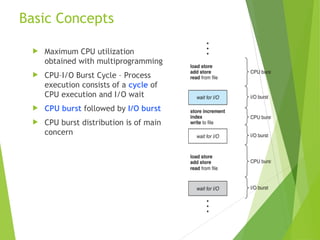
2. Basic Concepts
 Maximum CPU utilization
obtained with multiprogramming
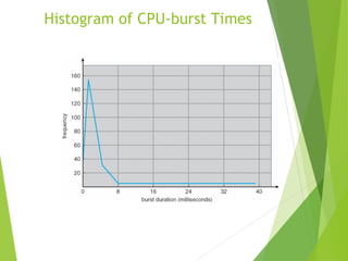
 CPU–I/O Burst Cycle – Process
execution consists of a cycle of
CPU execution and I/O wait
 CPU burst followed by I/O burst
 CPU burst distribution is of main
concern

3. Histogram of CPU-burst Times

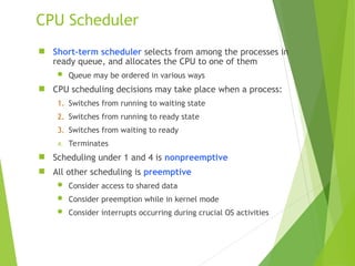
4. CPU Scheduler
 Short-term scheduler selects from among the processes in
ready queue, and allocates the CPU to one of them
 Queue may be ordered in various ways
 CPU scheduling decisions may take place when a process:
1. Switches from running to waiting state
2. Switches from running to ready state
3. Switches from waiting to ready
4. Terminates
 Scheduling under 1 and 4 is nonpreemptive
 All other scheduling is preemptive
 Consider access to shared data
 Consider preemption while in kernel mode
 Consider interrupts occurring during crucial OS activities

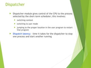
5. Dispatcher
 Dispatcher module gives control of the CPU to the process
selected by the short-term scheduler; this involves:
 switching context
 switching to user mode
 jumping to the proper location in the user program to restart
that program
 Dispatch latency – time it takes for the dispatcher to stop
one process and start another running

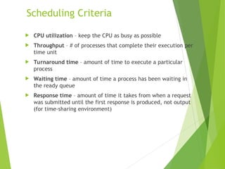
6. Scheduling Criteria
 CPU utilization – keep the CPU as busy as possible
 Throughput – # of processes that complete their execution per
time unit
 Turnaround time – amount of time to execute a particular
process
 Waiting time – amount of time a process has been waiting in
the ready queue
 Response time – amount of time it takes from when a request
was submitted until the first response is produced, not output
(for time-sharing environment)

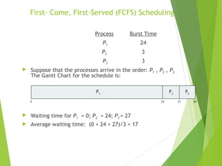
7. First- Come, First-Served (FCFS) Scheduling
Process Burst Time
P1 24
P2 3
P3 3
 Suppose that the processes arrive in the order: P1 , P2 , P3
The Gantt Chart for the schedule is:
 Waiting time for P1 = 0; P2 = 24; P3 = 27
 Average waiting time: (0 + 24 + 27)/3 = 17
P P P
1 2 3
0 24 30
27

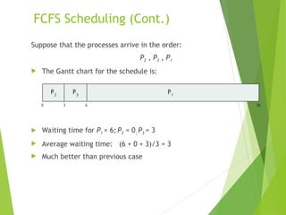
8. FCFS Scheduling (Cont.)
Suppose that the processes arrive in the order:
P2 , P3 , P1
 The Gantt chart for the schedule is:
 Waiting time for P1 = 6; P2 = 0; P3 = 3
 Average waiting time: (6 + 0 + 3)/3 = 3
 Much better than previous case
P1
0 3 6 30
P2
P3

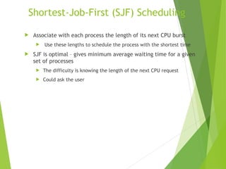
9. Shortest-Job-First (SJF) Scheduling
 Associate with each process the length of its next CPU burst
 Use these lengths to schedule the process with the shortest time
 SJF is optimal – gives minimum average waiting time for a given
set of processes
 The difficulty is knowing the length of the next CPU request
 Could ask the user

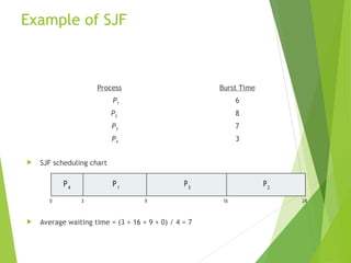
10. Example of SJF
ProcessArriva l Time Burst Time
P1 0.0 6
P2 2.0 8
P3 4.0 7
P4 5.0 3
 SJF scheduling chart
 Average waiting time = (3 + 16 + 9 + 0) / 4 = 7
P3
0 3 24
P4
P1
16
9
P2

11. Example of Shortest-remaining-time-first
 Now we add the concepts of varying arrival times and preemption to the
analysis
ProcessAarri Arrival TimeTBurst Time
P1 0 8
P2 1 4
P3 2 9
P4 3 5
 Preemptive SJF Gantt Chart
 Average waiting time = [(10-1)+(1-1)+(17-2)+5-3)]/4 = 26/4 = 6.5 msec
P4
0 1 26
P1
P2
10
P3
P1
5 17

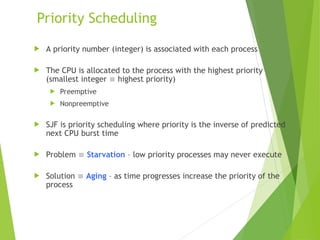
12. Priority Scheduling
 A priority number (integer) is associated with each process
 The CPU is allocated to the process with the highest priority
(smallest integer  highest priority)
 Preemptive
 Nonpreemptive
 SJF is priority scheduling where priority is the inverse of predicted
next CPU burst time
 Problem  Starvation – low priority processes may never execute
 Solution  Aging – as time progresses increase the priority of the
process

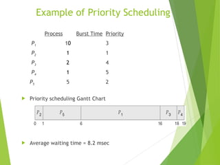
13. Example of Priority Scheduling
ProcessAarri Burst TimeTPriority
P1 10 3
P2 1 1
P3 2 4
P4 1 5
P5 5 2
 Priority scheduling Gantt Chart
 Average waiting time = 8.2 msec

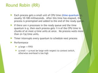
14. Round Robin (RR)
 Each process gets a small unit of CPU time (time quantum q),
usually 10-100 milliseconds. After this time has elapsed, the
process is preempted and added to the end of the ready queue.
 If there are n processes in the ready queue and the time
quantum is q, then each process gets 1/n of the CPU time in
chunks of at most q time units at once. No process waits more
than (n-1)q time units.
 Timer interrupts every quantum to schedule next process
 Performance
 q large  FIFO
 q small  q must be large with respect to context switch,
otherwise overhead is too high

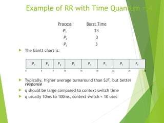
15. Example of RR with Time Quantum = 4
Process Burst Time
P1 24
P2 3
P3 3
 The Gantt chart is:
 Typically, higher average turnaround than SJF, but better
response
 q should be large compared to context switch time
 q usually 10ms to 100ms, context switch < 10 usec
P P P
1 1 1
0 18 30
26
14
4 7 10 22
P2
P3
P1
P1
P1

16. Time Quantum and Context Switch Time

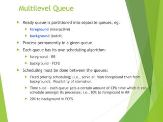
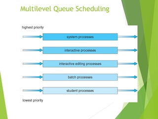
17. Multilevel Queue
 Ready queue is partitioned into separate queues, eg:
 foreground (interactive)
 background (batch)
 Process permanently in a given queue
 Each queue has its own scheduling algorithm:
 foreground – RR
 background – FCFS
 Scheduling must be done between the queues:
 Fixed priority scheduling; (i.e., serve all from foreground then from
background). Possibility of starvation.
 Time slice – each queue gets a certain amount of CPU time which it can
schedule amongst its processes; i.e., 80% to foreground in RR
 20% to background in FCFS

18. Multilevel Queue Scheduling

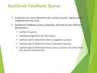
19. Multilevel Feedback Queue
 A process can move between the various queues; aging can be
implemented this way
 Multilevel-feedback-queue scheduler defined by the following
parameters:
 number of queues
 scheduling algorithms for each queue
 method used to determine when to upgrade a process
 method used to determine when to demote a process
 method used to determine which queue a process will enter when
that process needs service

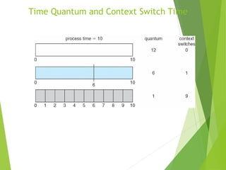
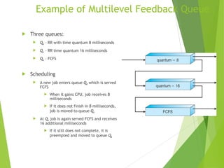
20. Example of Multilevel Feedback Queue
 Three queues:
 Q0 – RR with time quantum 8 milliseconds
 Q1 – RR time quantum 16 milliseconds
 Q2 – FCFS
 Scheduling
 A new job enters queue Q0 which is served
FCFS
 When it gains CPU, job receives 8
milliseconds
 If it does not finish in 8 milliseconds,
job is moved to queue Q1
 At Q1 job is again served FCFS and receives
16 additional milliseconds
 If it still does not complete, it is
preempted and moved to queue Q2