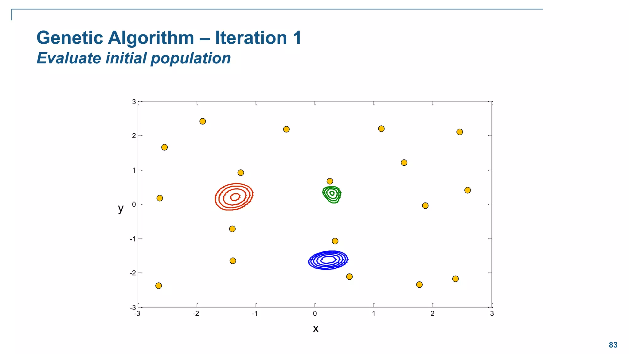
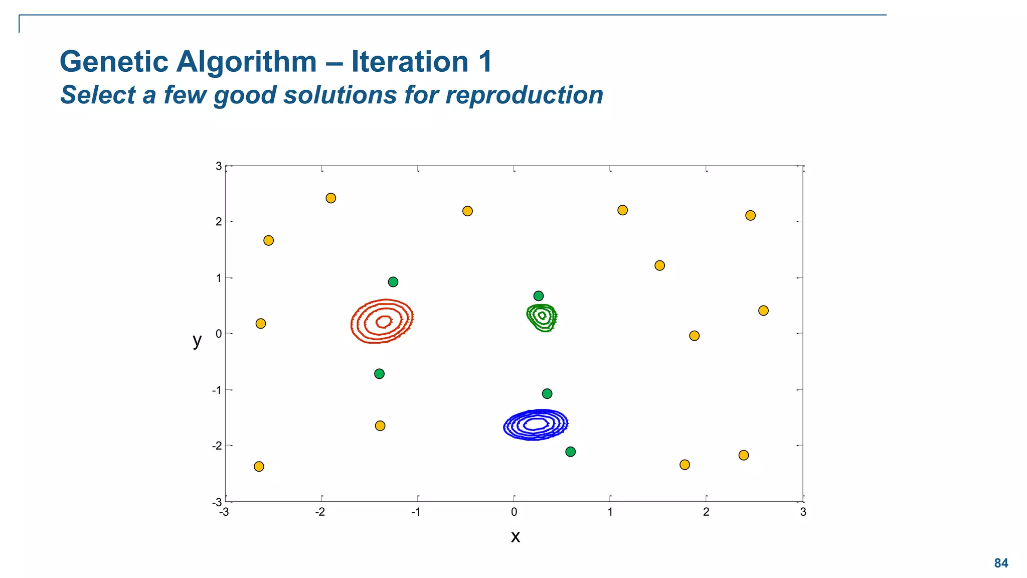
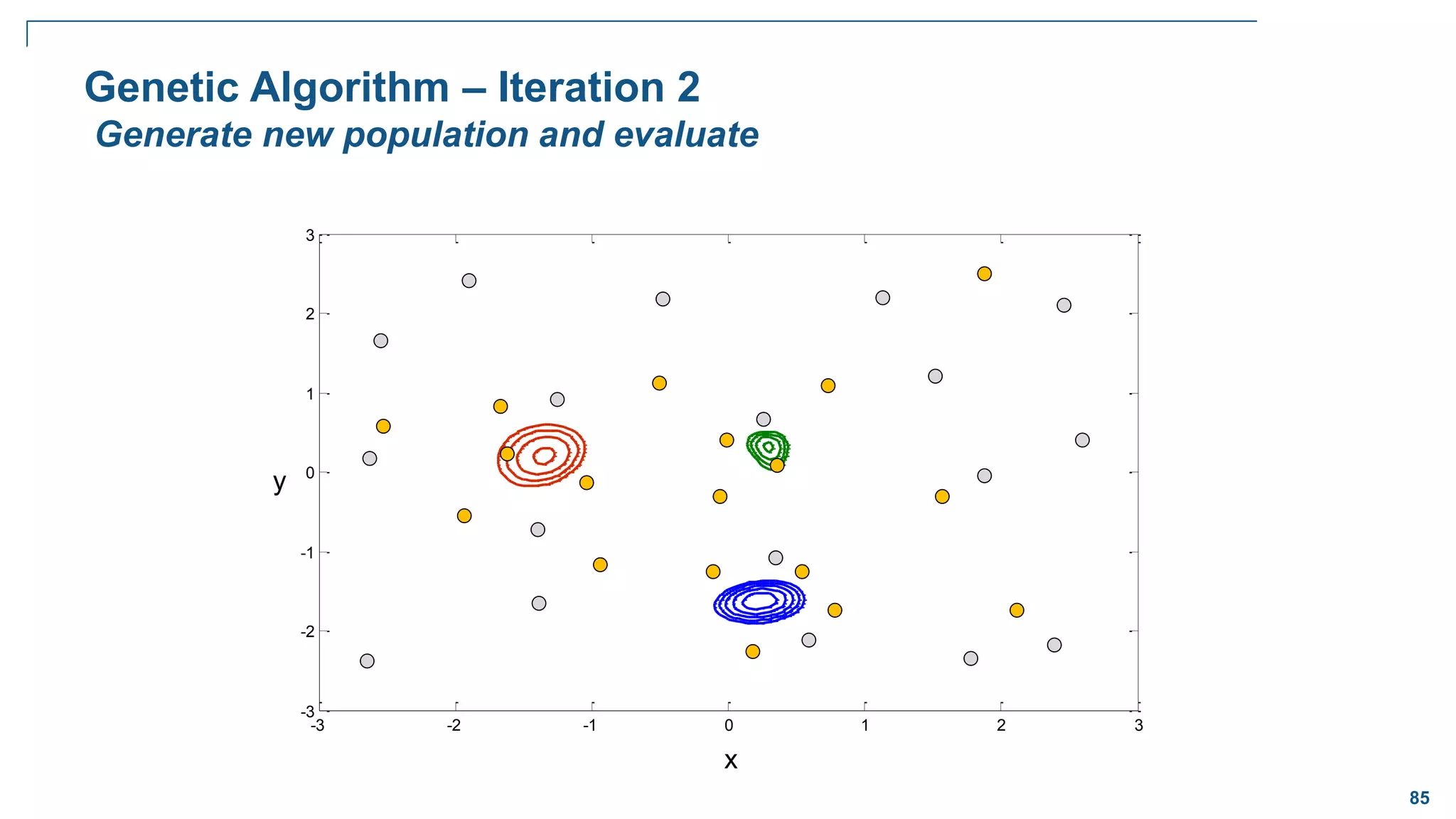
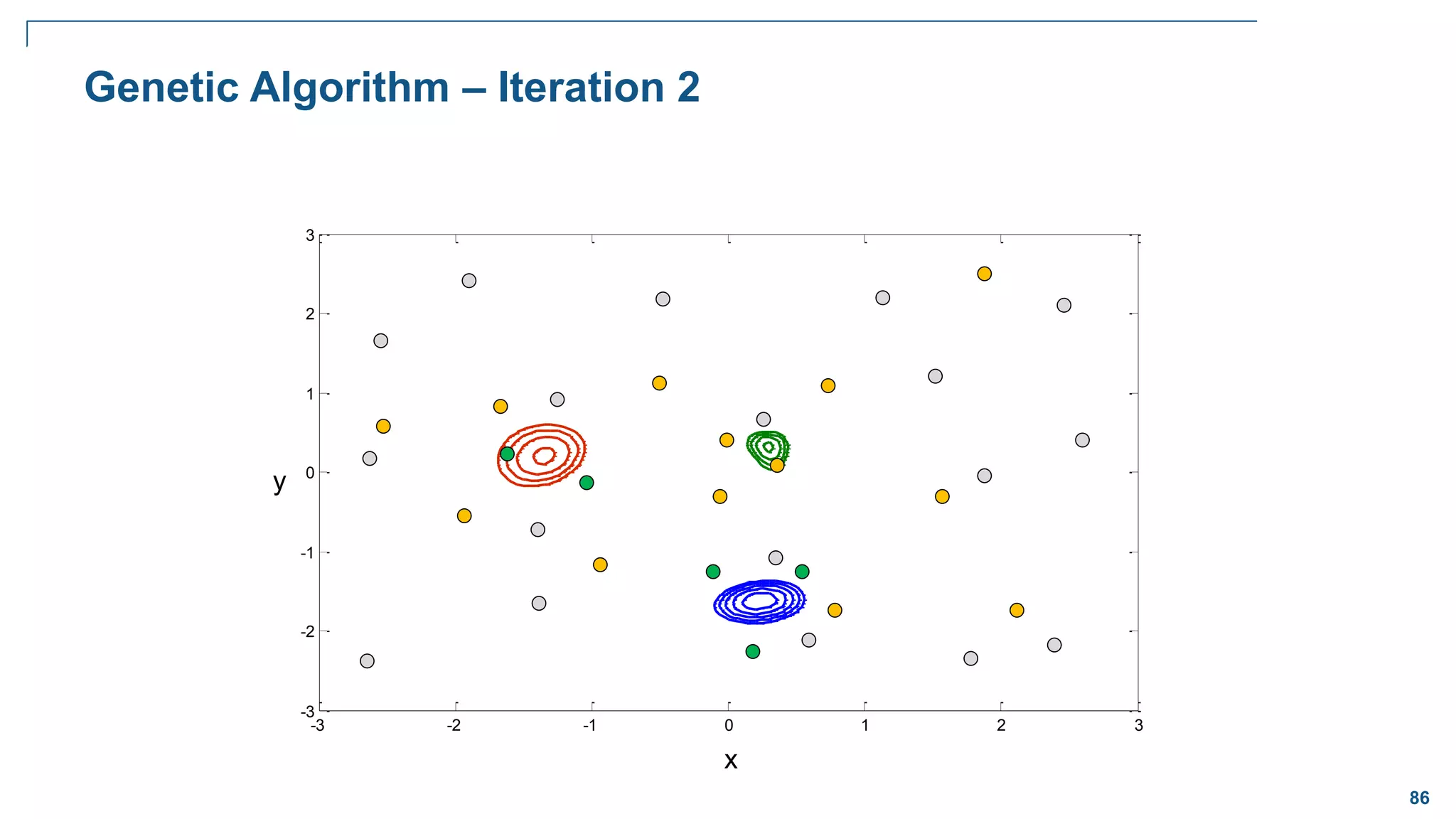
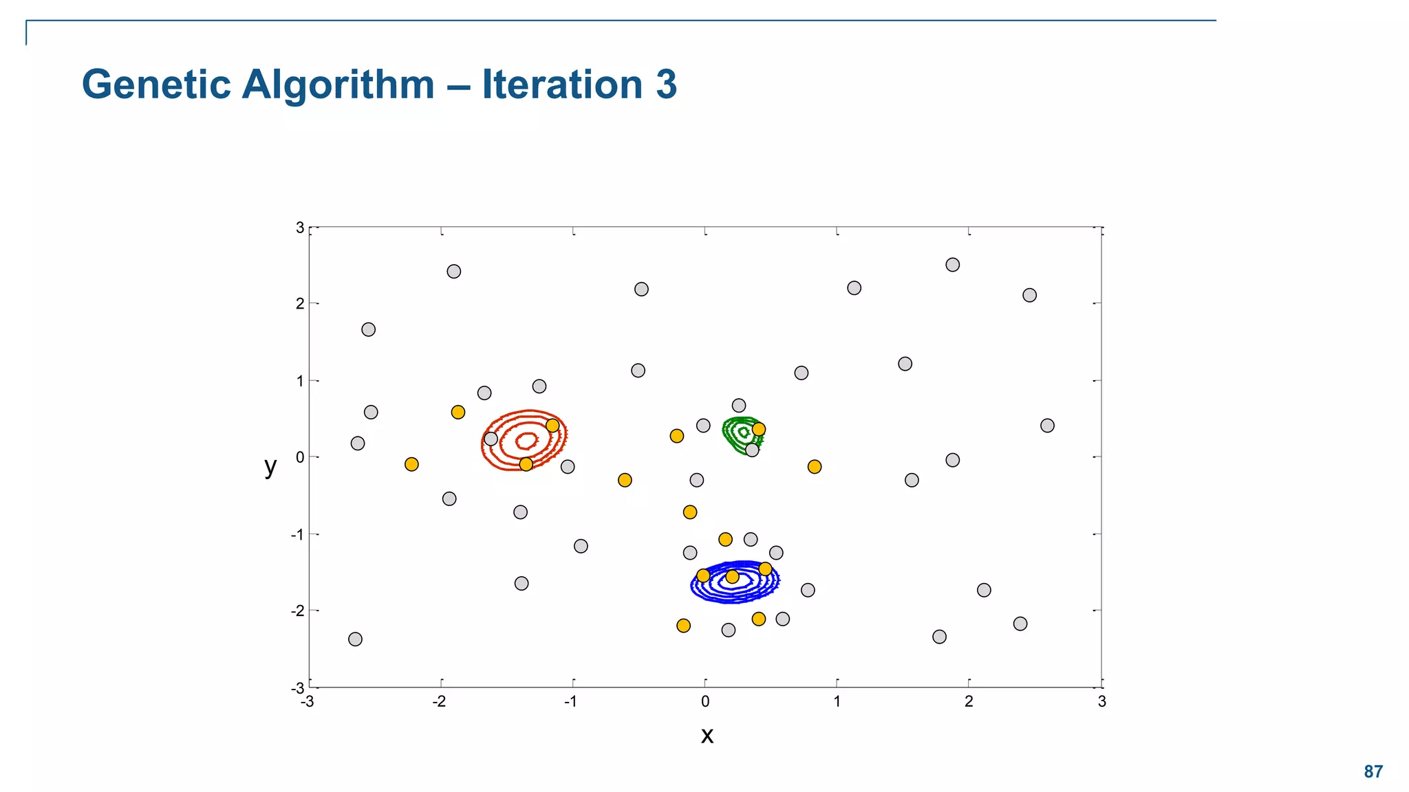
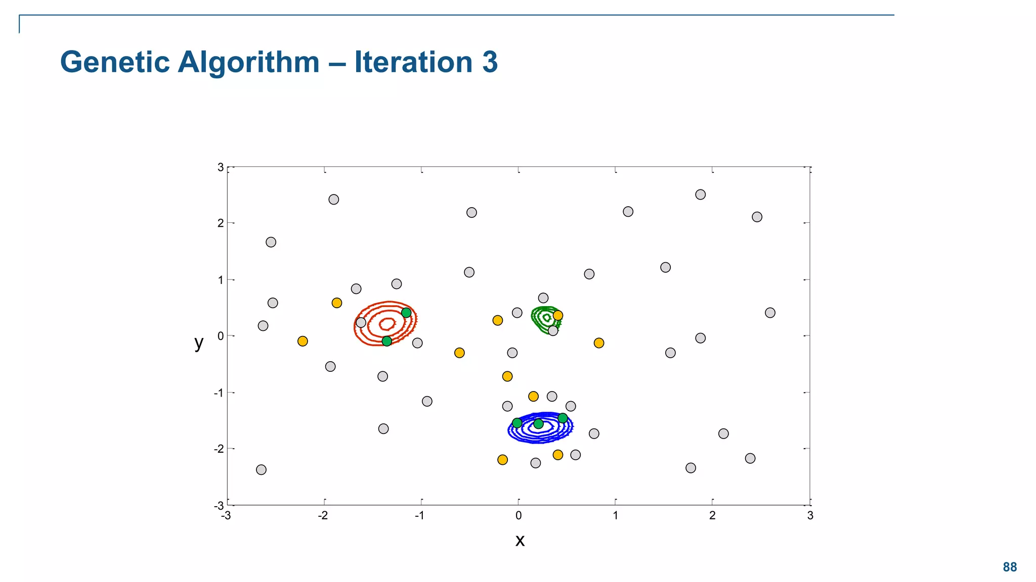
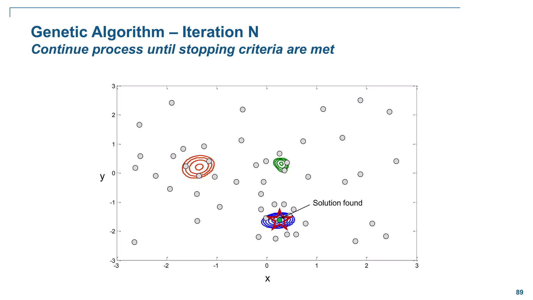
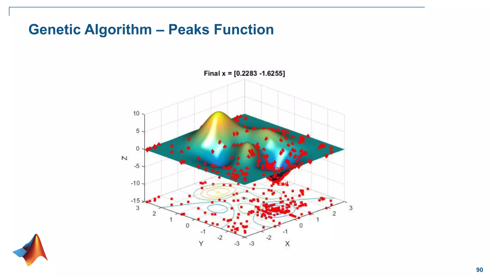
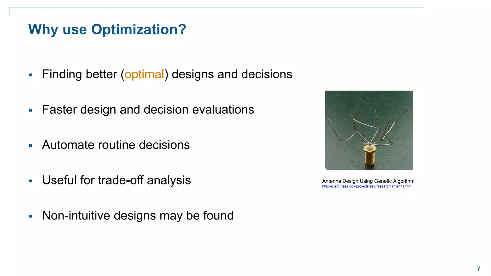
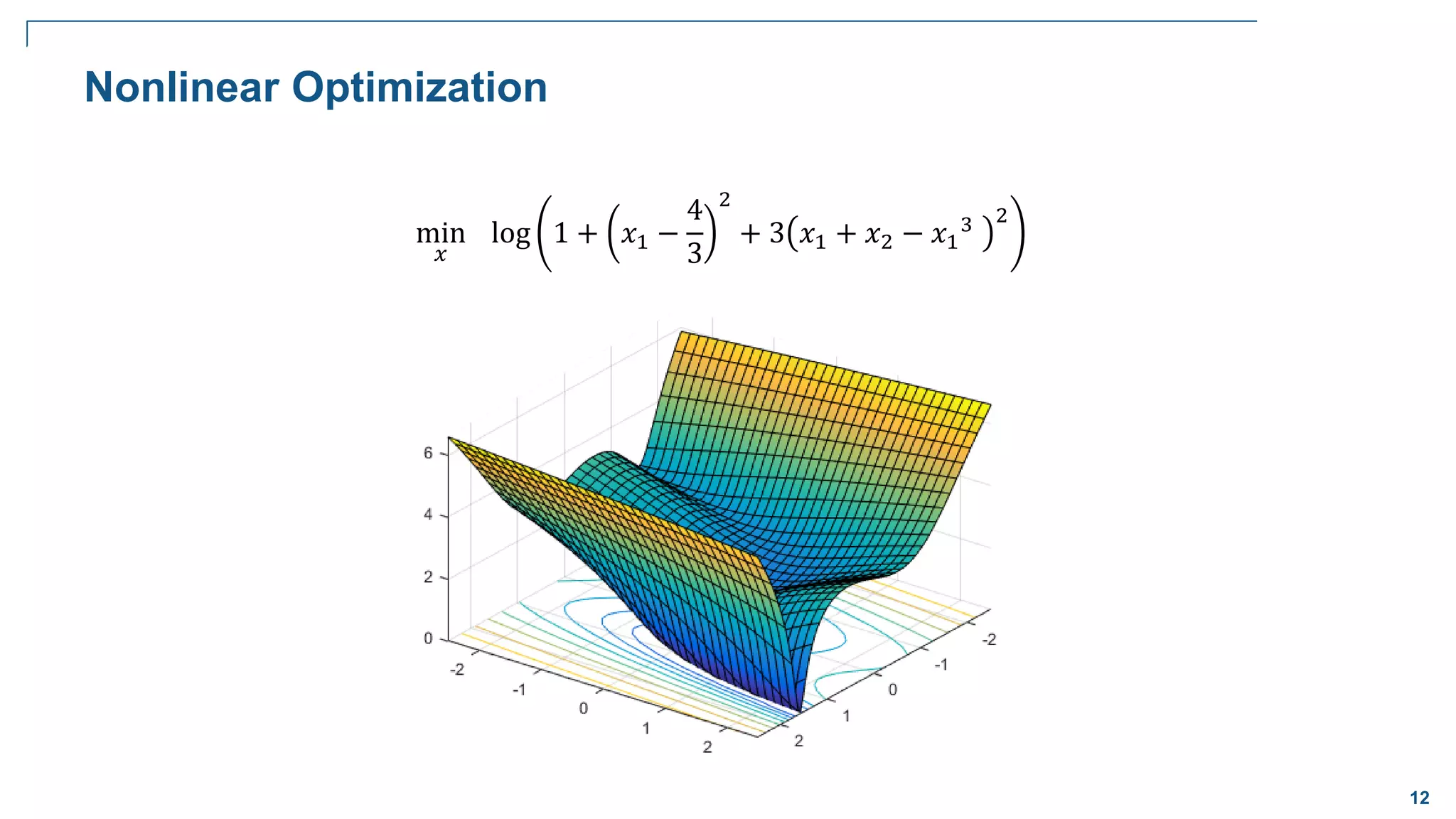
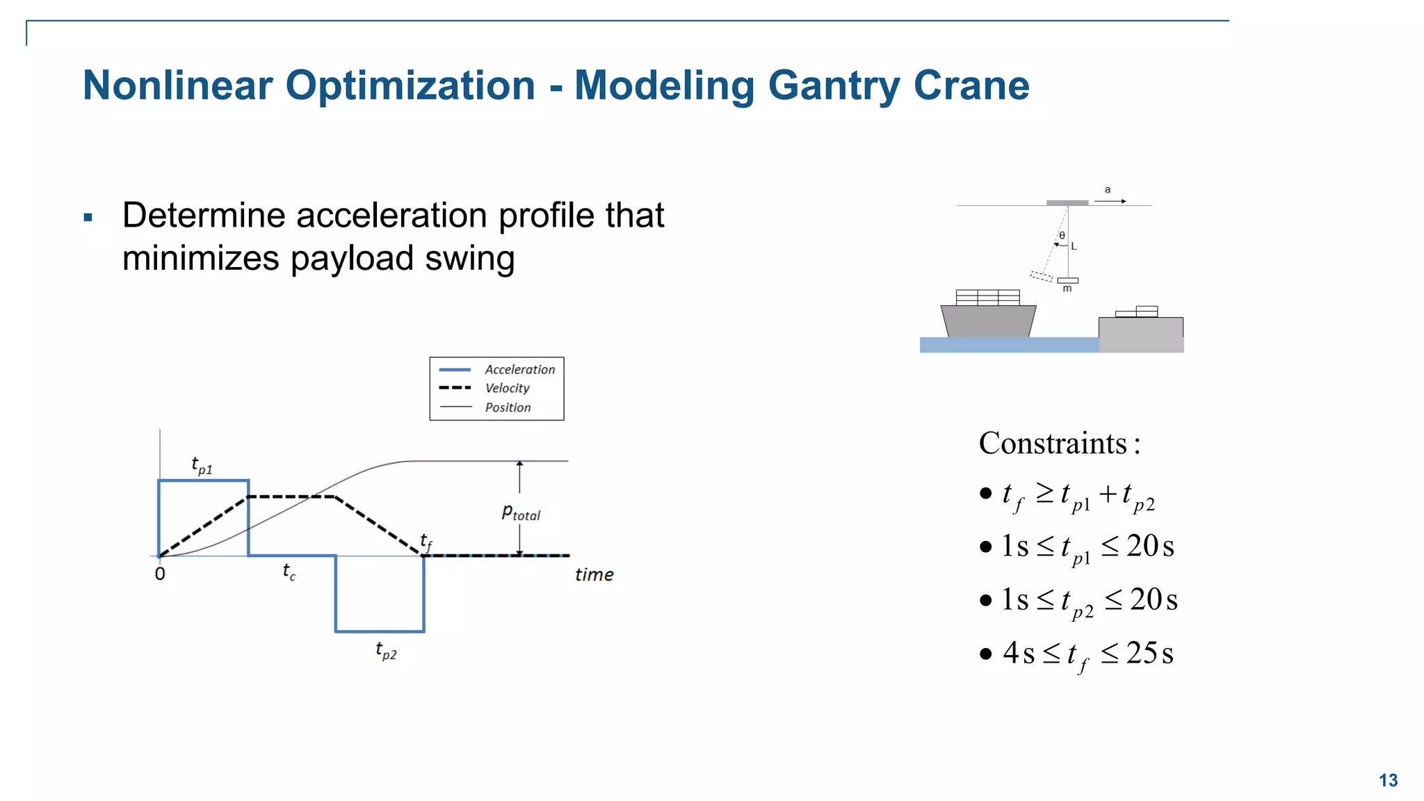
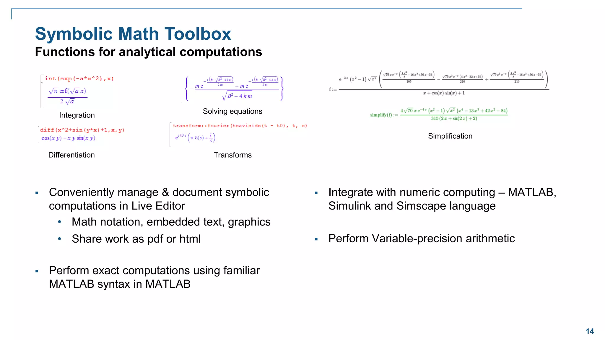
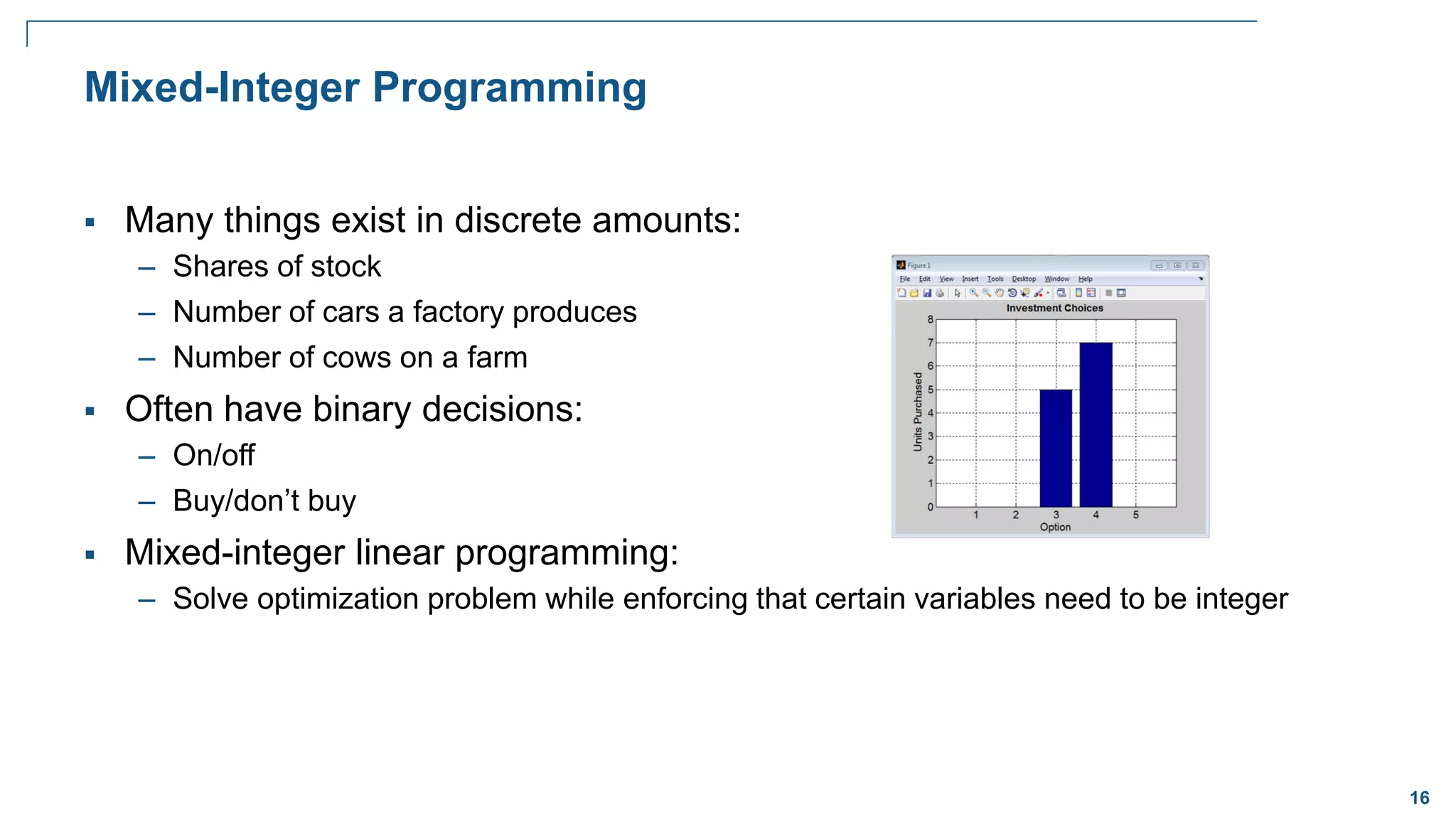
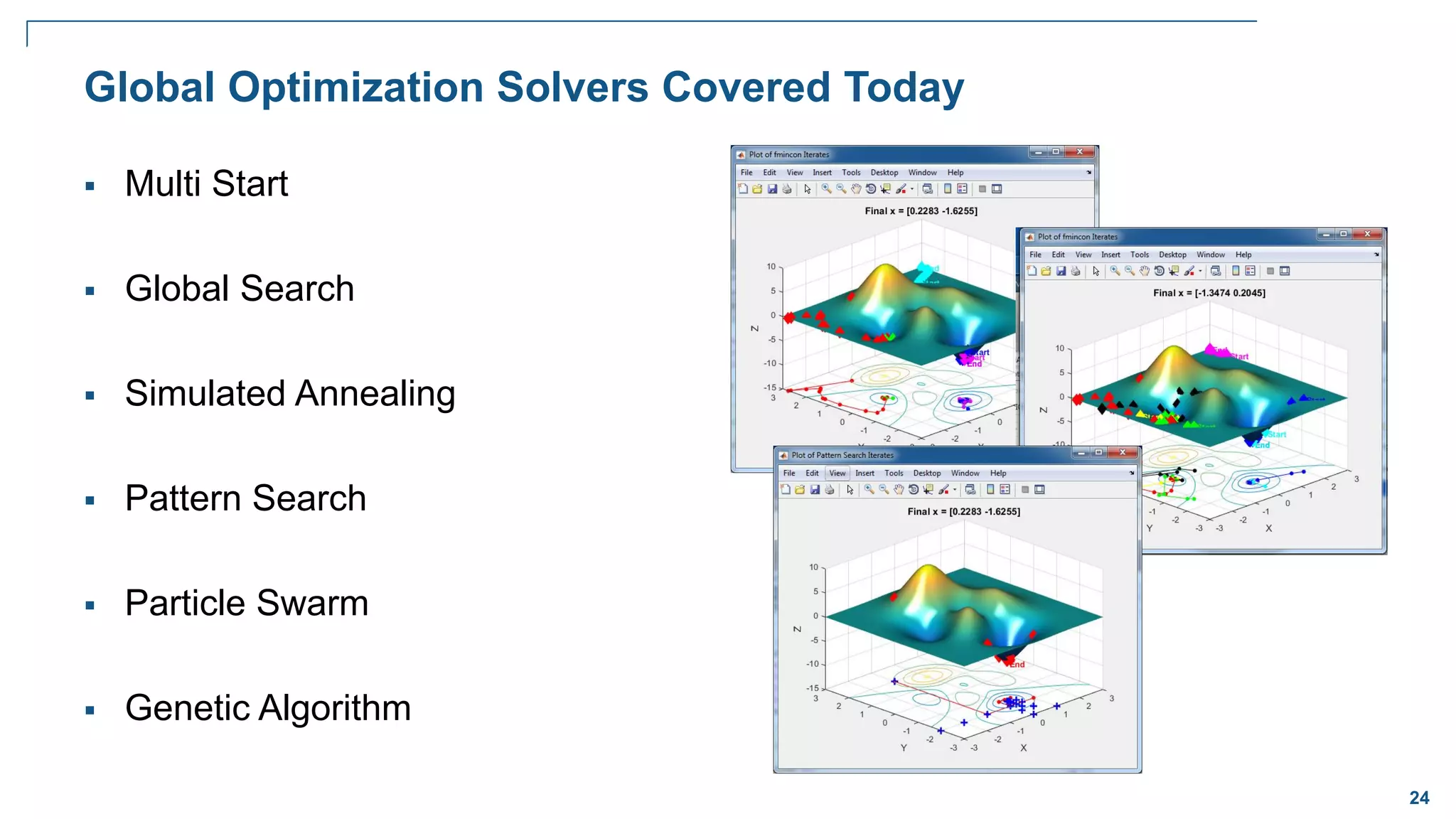
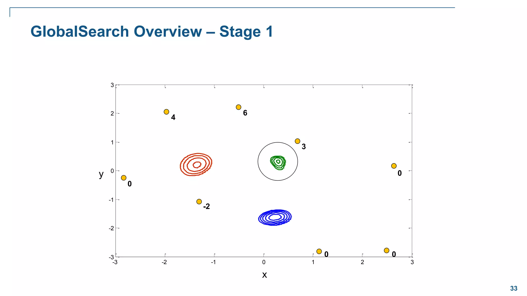
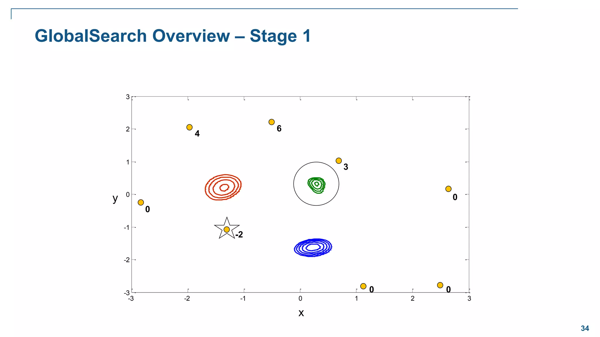
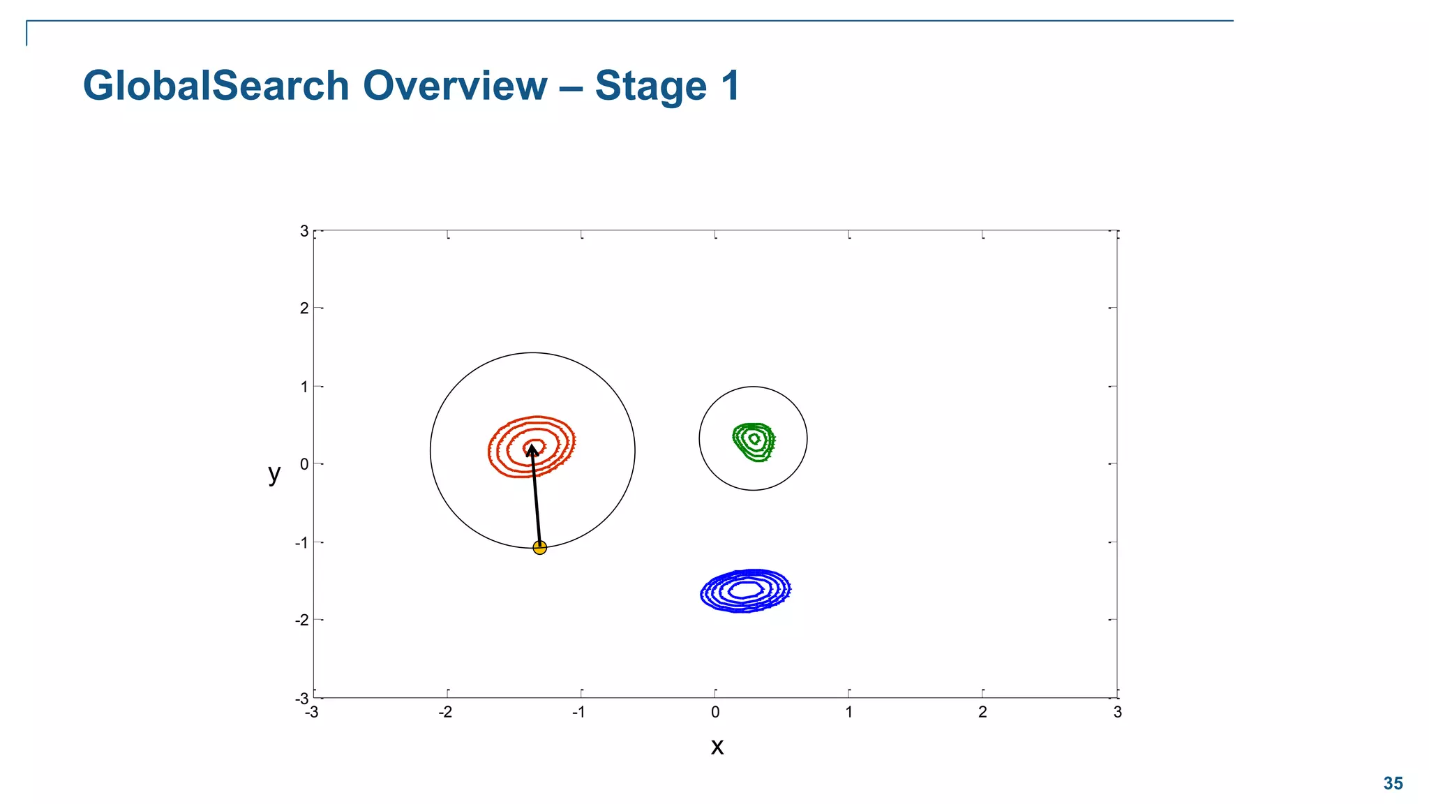
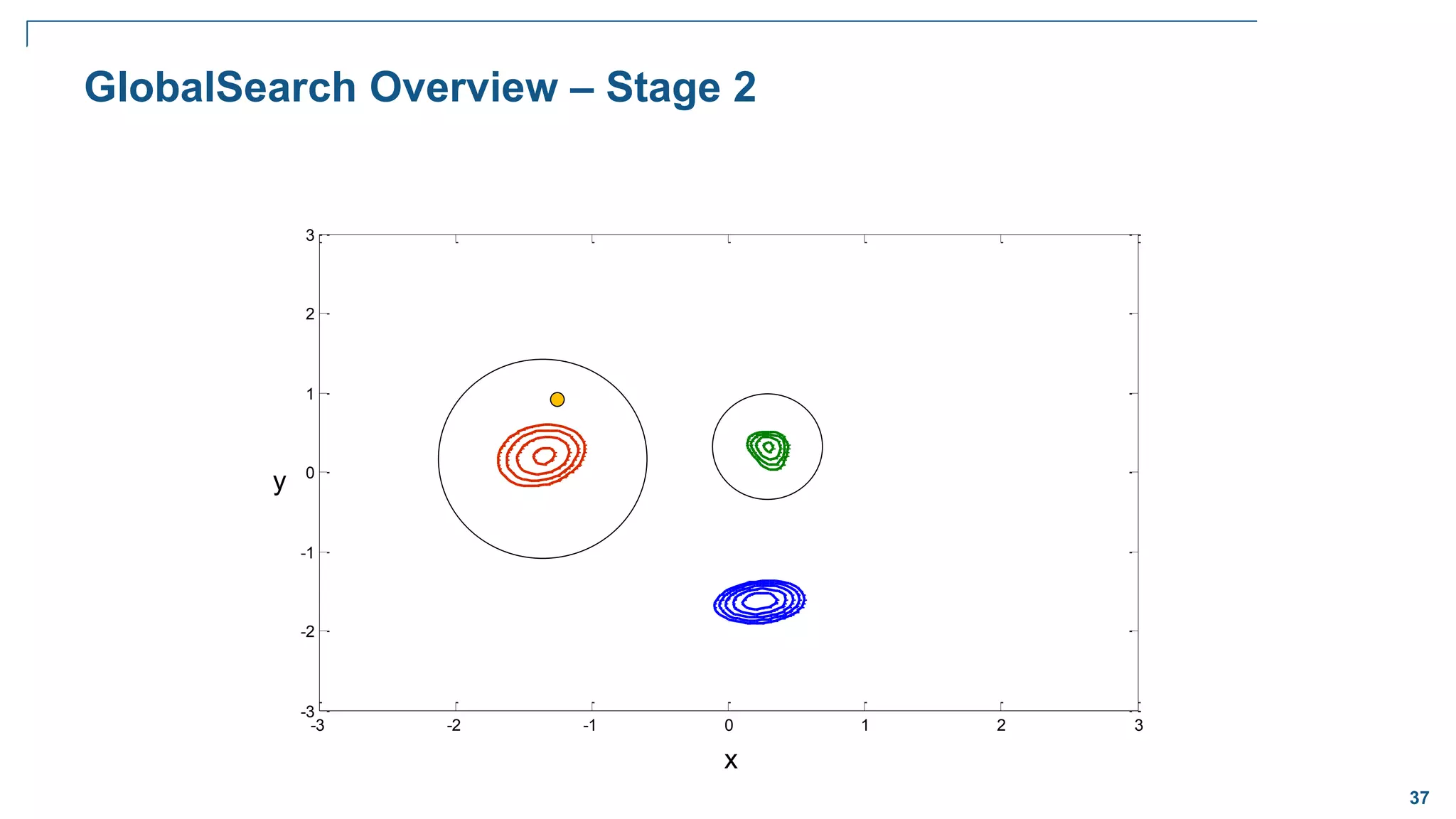
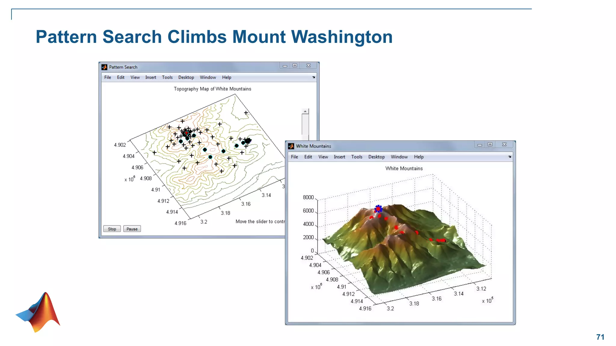
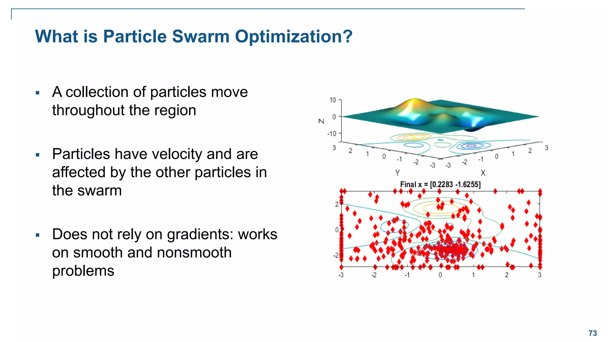
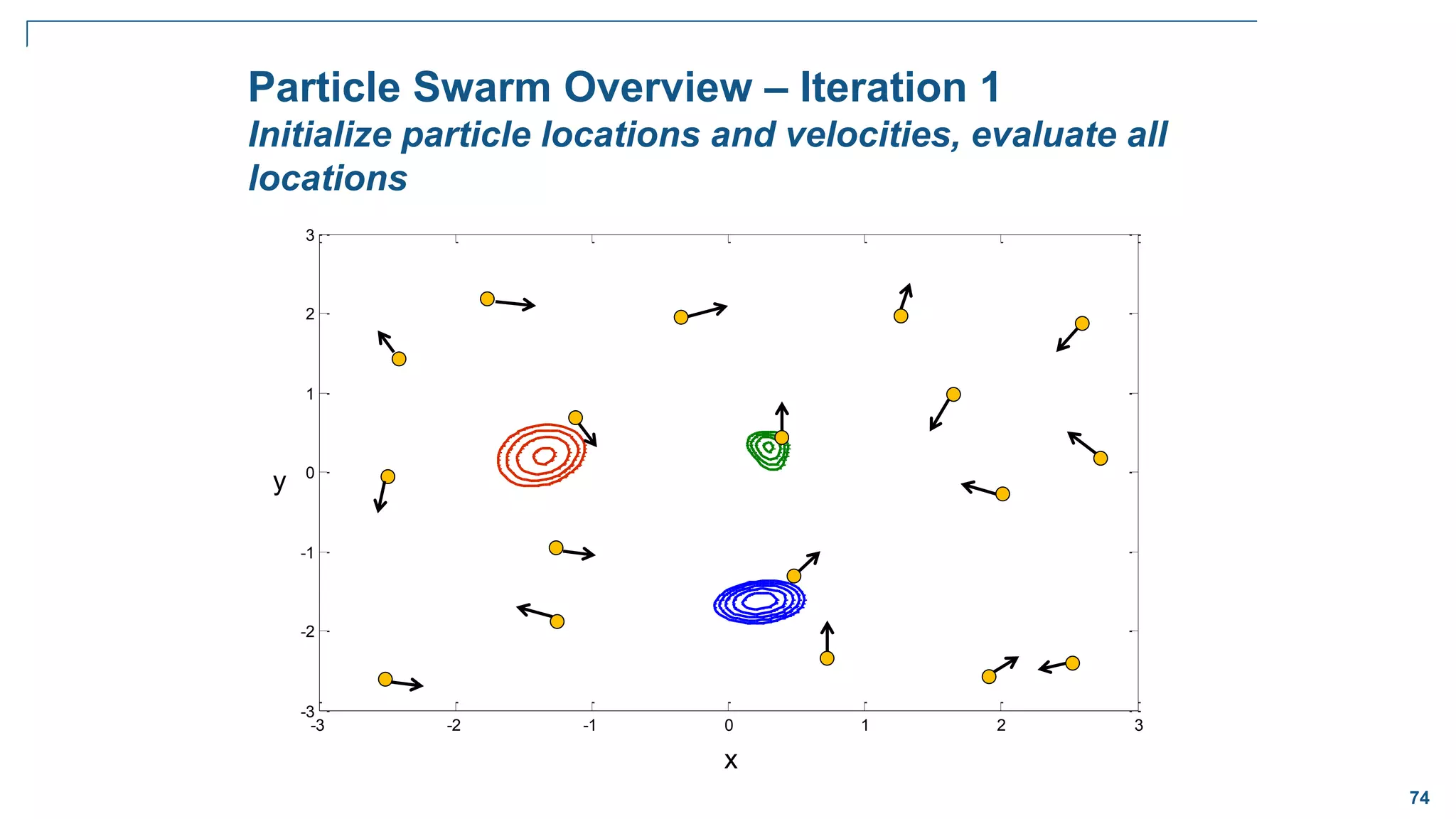
The document discusses various optimization techniques in MATLAB, including least squares minimization, nonlinear optimization, mixed-integer programming, and global optimization. It provides examples of curve fitting, nonlinear function minimization, the traveling salesman problem, and global optimization techniques like multi-start, global search, simulated annealing, and particle swarm optimization.

1. Solving Optimization Problems with MATLAB

2. 2
 Introduction
 Least-squares minimization
 Nonlinear optimization
 Mixed-integer programming
 Global optimization
Topics

3. 3
Optimization Problems
Minimize Risk
Maximize Profits
Maximize Fuel Efficiency

4. 4
Design Process
Initial
Design
Variables
System
Modify
Design
Variables
Optimal
Design
Objectives
met?
No
Yes

5. 5
Manually (trial-and-error or iteratively)
Why use Optimization?
Initial
Guess

6. 6
Automatically (using optimization techniques)
Initial
Guess
Why use Optimization?

7. 7
Why use Optimization?
 Finding better (optimal) designs and decisions
 Faster design and decision evaluations
 Automate routine decisions
 Useful for trade-off analysis
 Non-intuitive designs may be found
Antenna Design Using Genetic Algorithm
http://ic.arc.nasa.gov/projects/esg/research/antenna.htm

8. 8
 Introduction
 Least-squares minimization
 Nonlinear optimization
 Mixed-integer programming
 Global optimization
Topics

9. 9
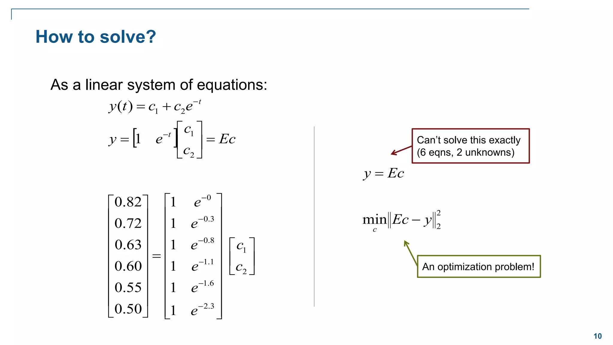
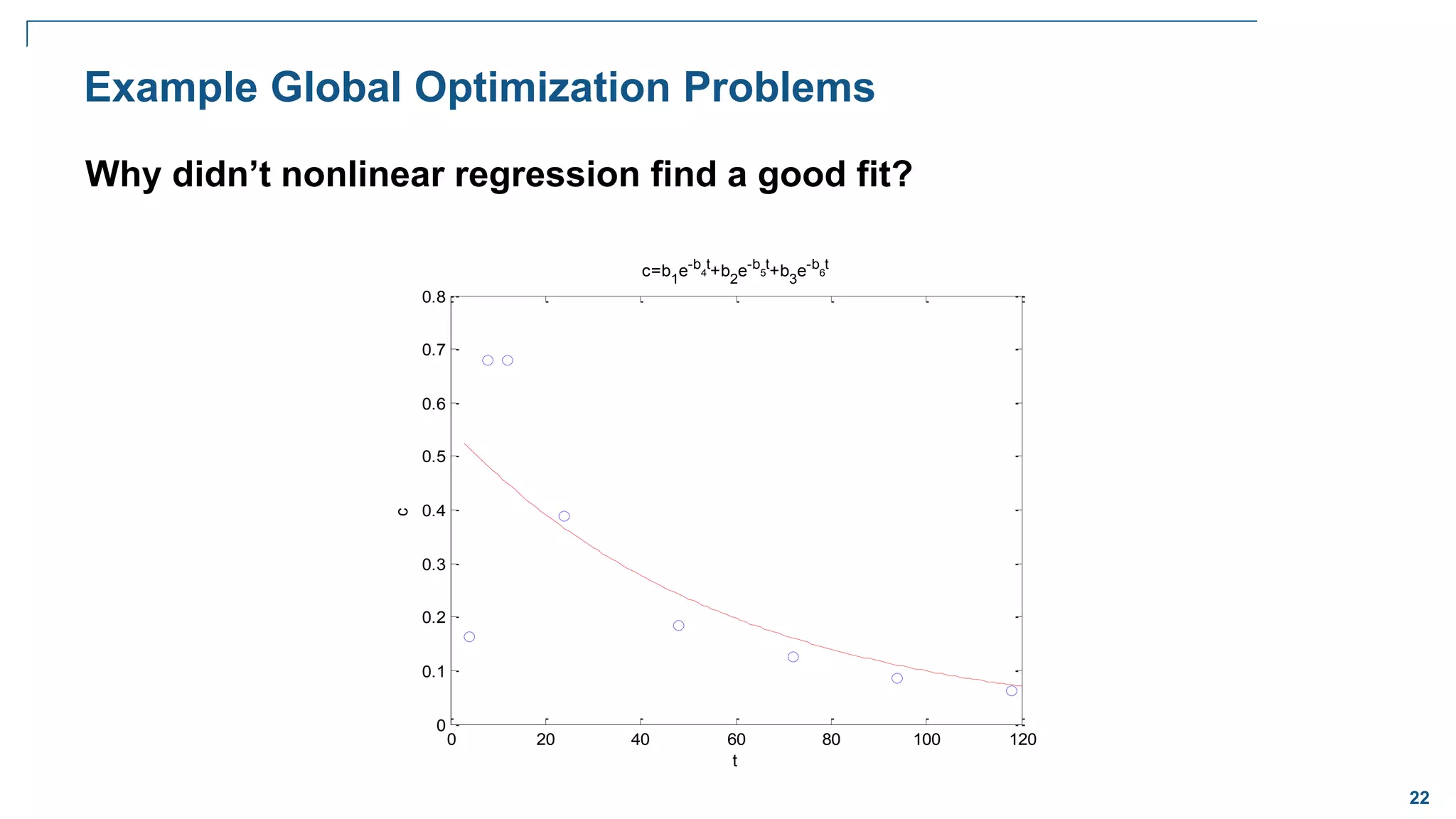
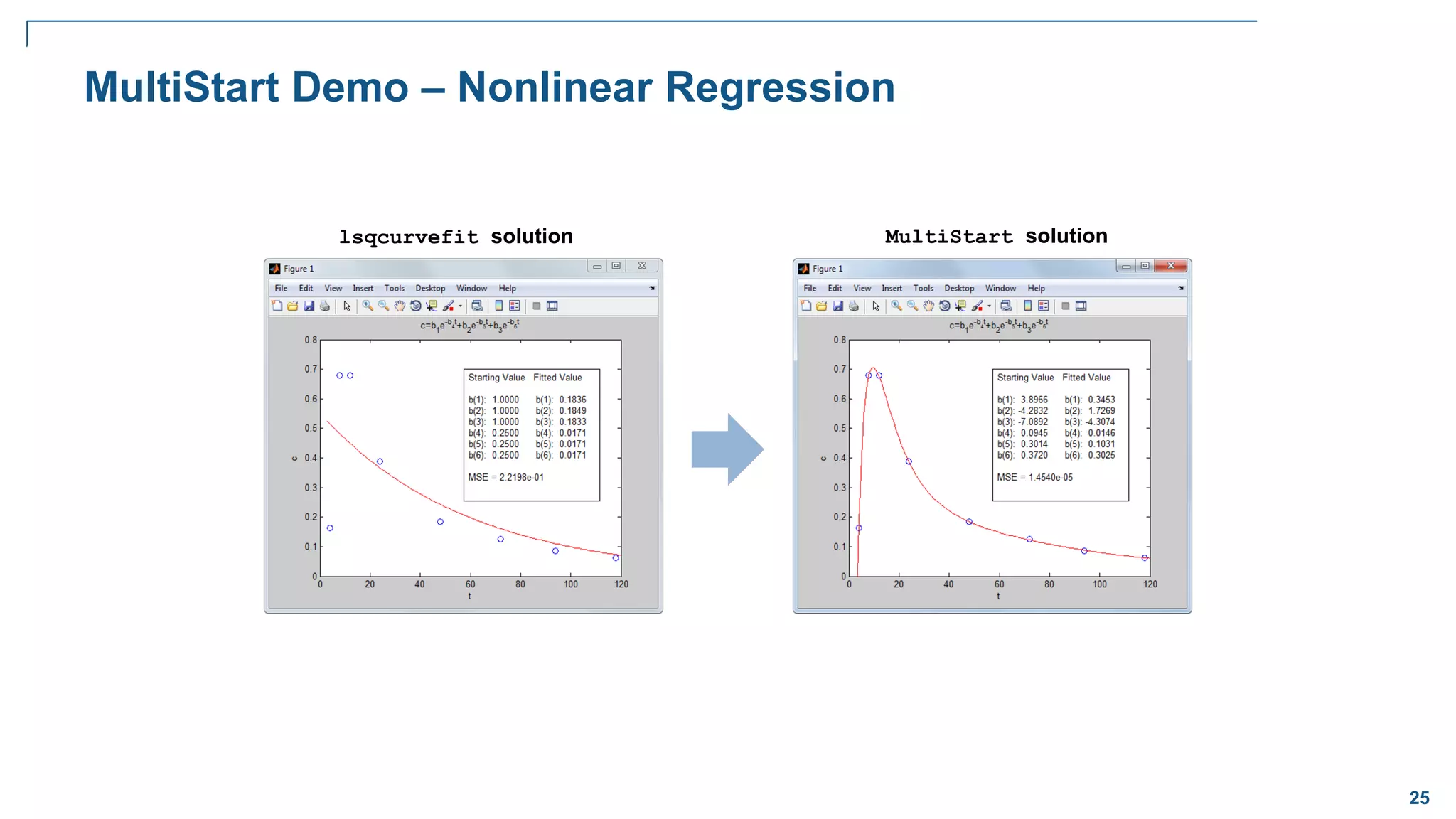
Curve Fitting Demo
Given some data:
Fit a curve of the form:
t
e
c
c
t
y 

 2
1
)
(
t = [0 .3 .8 1.1 1.6 2.3];
y = [.82 .72 .63 .60 .55 .50];

10. 10
How to solve?
  Ec
c
c
e
y
e
c
c
t
y
t
t












2
1
2
1
1
)
(
As a linear system of equations:
2
2
min y
Ec
Ec
y
c


Can’t solve this exactly
(6 eqns, 2 unknowns)
An optimization problem!



















































2
1
3
.
2
6
.
1
1
.
1
8
.
0
3
.
0
0
1
1
1
1
1
1
50
.
0
55
.
0
60
.
0
63
.
0
72
.
0
82
.
0
c
c
e
e
e
e
e
e

11. 11
 Introduction
 Least-squares minimization
 Nonlinear optimization
 Mixed-integer programming
 Global optimization
Topics

12. 12
Nonlinear Optimization
min
𝑥
log 1 + 𝑥1 −
4
3
2
+ 3 𝑥1 + 𝑥2 − 𝑥1
3 2

13. 13
Nonlinear Optimization - Modeling Gantry Crane
 Determine acceleration profile that
minimizes payload swing
s
25
s
4
s
20
s
1
s
20
s
1
:
s
Constraint
2
1
2
1












f
p
p
p
p
f
t
t
t
t
t
t

14. 14
Symbolic Math Toolbox
Functions for analytical computations
 Conveniently manage & document symbolic
computations in Live Editor
• Math notation, embedded text, graphics
• Share work as pdf or html
 Perform exact computations using familiar
MATLAB syntax in MATLAB
Integration
Differentiation
Solving equations
Transforms
Simplification
 Integrate with numeric computing – MATLAB,
Simulink and Simscape language
 Perform Variable-precision arithmetic

15. 15
 Introduction
 Least-squares minimization
 Nonlinear optimization
 Mixed-integer programming
 Global optimization
Topics

16. 16
Mixed-Integer Programming
 Many things exist in discrete amounts:
– Shares of stock
– Number of cars a factory produces
– Number of cows on a farm
 Often have binary decisions:
– On/off
– Buy/don’t buy
 Mixed-integer linear programming:
– Solve optimization problem while enforcing that certain variables need to be integer

17. 17
Continuous and integer variables
𝑥1 ∈ 0, 100 𝑥2 ∈ {1,2,3,4,5}
Linear objective and constraints
min
𝑥
−𝑥1 − 2𝑥2
𝑥1 + 4𝑥2 ≤ 20
𝑥1 + 𝑥2 = 10
such that
Mixed-Integer Linear Programming

18. 18
Traveling Salesman Problem
Problem
 How to find the shortest path through a series of points?
Solution
 Calculate distances between all combinations of points
 Solve an optimization problem where variables correspond to trips between two points
1
1
1
0
1
1
0
0
0
0

19. 19
 Introduction
 Least-squares minimization
 Nonlinear optimization
 Mixed-integer programming
 Global optimization
Topics

20. 20
Example Global Optimization Problems
Why does fmincon have a hard time finding the
function minimum?
0 5 10
-10
-5
0
5
10
x
Starting at 10
0 5 10
-10
-5
0
5
10
x
Starting at 8
0 5 10
-10
-5
0
5
10
x
Starting at 6
x
sin(x)
+
x
cos(2
x)
0 5 10
-10
-5
0
5
10
x
Starting at 3
0 5 10
-10
-5
0
5
10
x
Starting at 1
0 5 10
-10
-5
0
5
10
x
Starting at 0
x
sin(x)
+
x
cos(2
x)

21. 21
Initial
Guess
Example Global Optimization Problems
Why didn’t fminunc find the maximum efficiency?

22. 22
Example Global Optimization Problems
Why didn’t nonlinear regression find a good fit?
0 20 40 60 80 100 120
0
0.1
0.2
0.3
0.4
0.5
0.6
0.7
0.8
t
c
c=b1
e-b
4
t
+b2
e-b
5
t
+b3
e-b
6
t

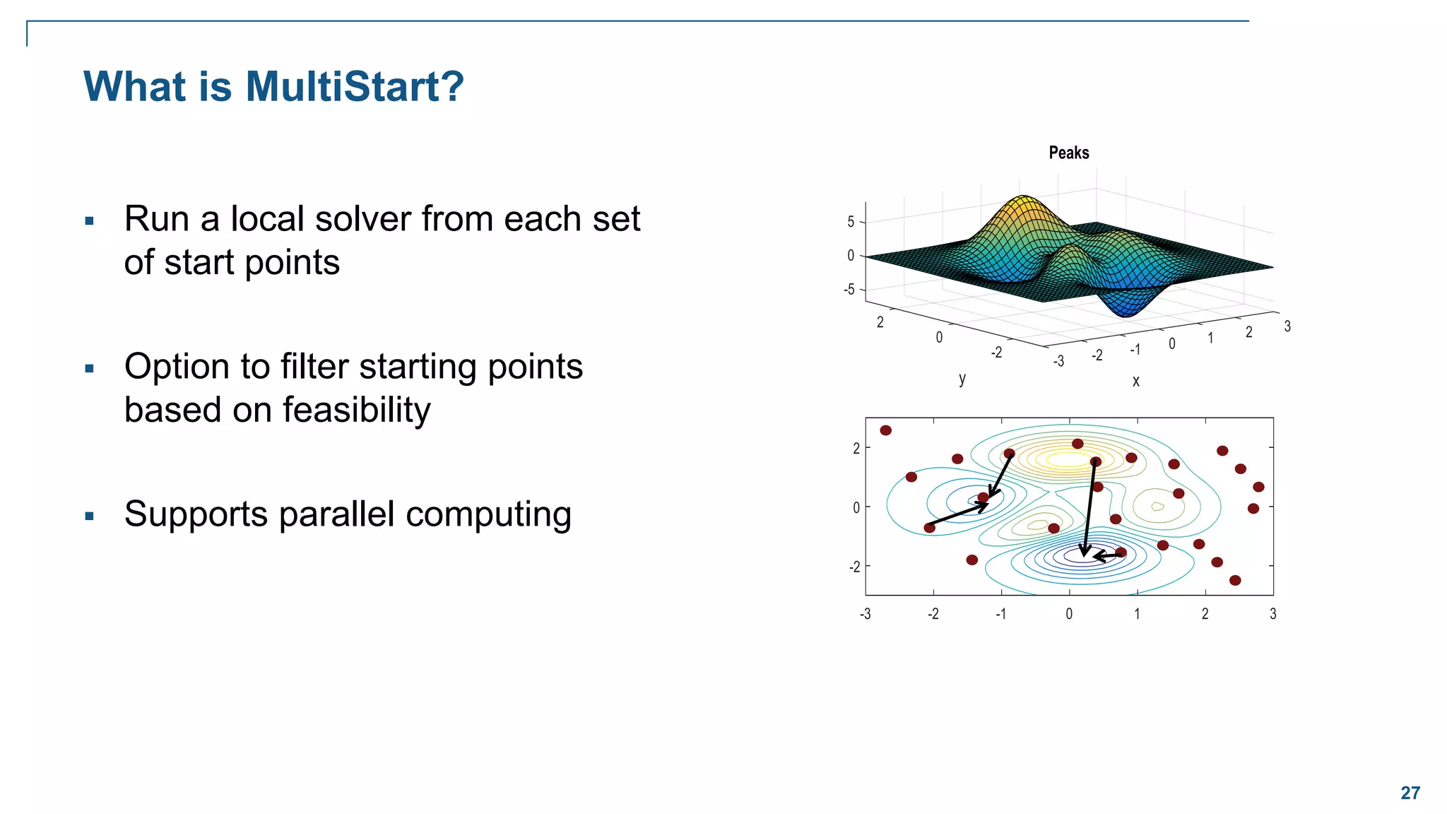
23. 23
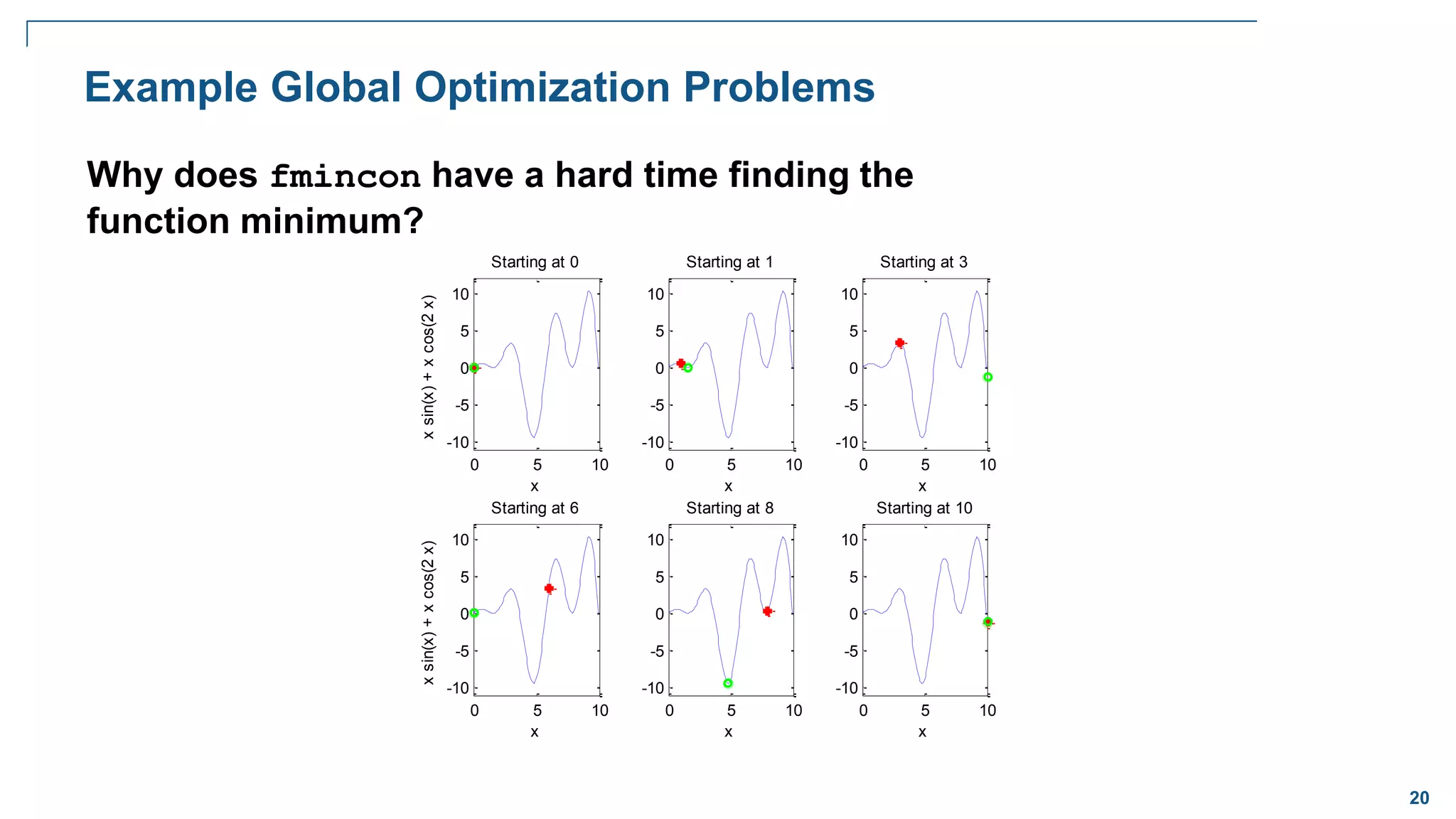
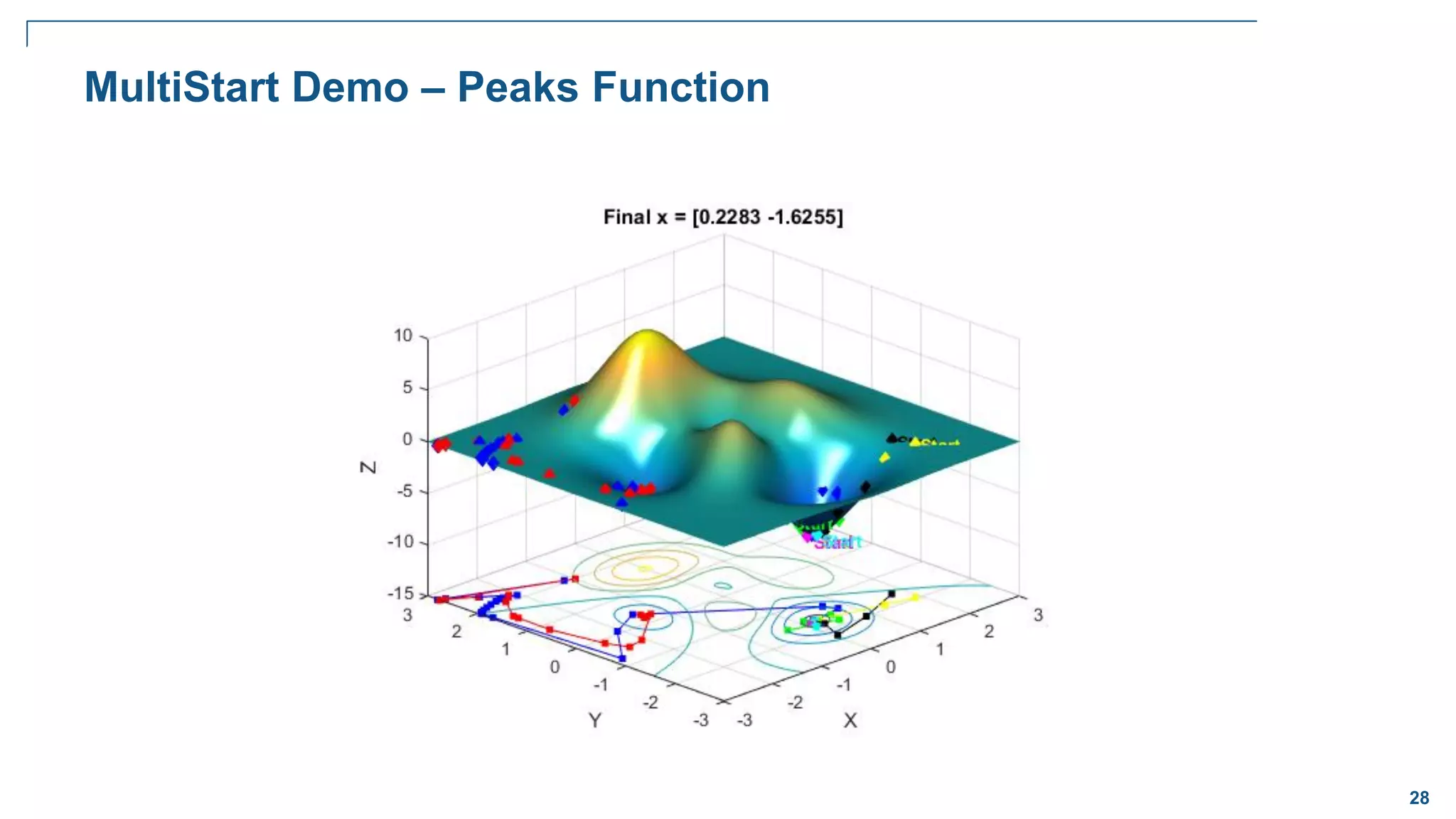
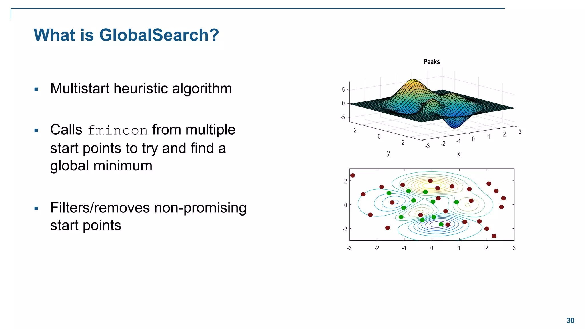
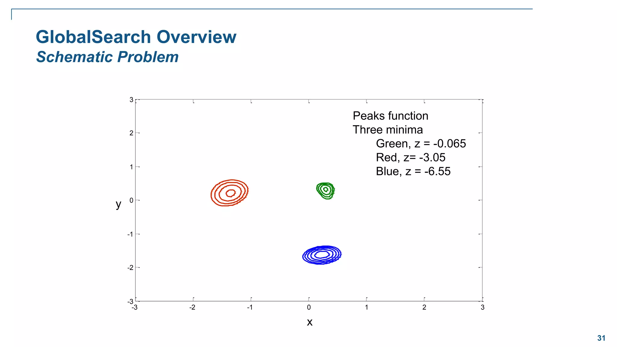
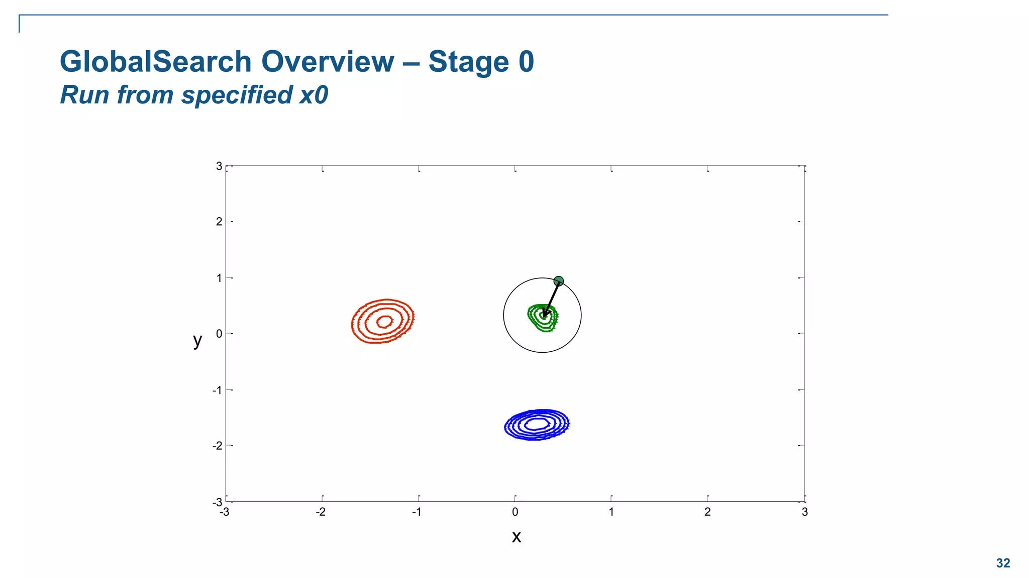
Global Optimization
Goal:
Want to find the lowest/largest value of
the nonlinear function that has many local
minima/maxima
Problem:
Traditional solvers often return one of the
local minima (not the global)
Solution:
A solver that locates globally optimal
solutions
Global Minimum at [0 0]
Rastrigin’s Function

24. 24
Global Optimization Solvers Covered Today
 Multi Start
 Global Search
 Simulated Annealing
 Pattern Search
 Particle Swarm
 Genetic Algorithm

25. 25
MultiStart Demo – Nonlinear Regression
lsqcurvefit solution MultiStart solution

26. 26
MULTISTART

27. 27
What is MultiStart?
 Run a local solver from each set
of start points
 Option to filter starting points
based on feasibility
 Supports parallel computing

28. 28
MultiStart Demo – Peaks Function

29. 29
GLOBAL SEARCH

30. 30
What is GlobalSearch?
 Multistart heuristic algorithm
 Calls fmincon from multiple
start points to try and find a
global minimum
 Filters/removes non-promising
start points

31. 31
-3 -2 -1 0 1 2 3
-3
-2
-1
0
1
2
3
GlobalSearch Overview
Schematic Problem
Peaks function
Three minima
Green, z = -0.065
Red, z= -3.05
Blue, z = -6.55
x
y

32. 32
-3 -2 -1 0 1 2 3
-3
-2
-1
0
1
2
3
GlobalSearch Overview – Stage 0
Run from specified x0
x
y

33. 33
-3 -2 -1 0 1 2 3
-3
-2
-1
0
1
2
3
GlobalSearch Overview – Stage 1
3
6
0
0
0
4
0
-2
x
y

34. 34
-3 -2 -1 0 1 2 3
-3
-2
-1
0
1
2
3
GlobalSearch Overview – Stage 1
3
6
0
0
0
4
0
-2
x
y

35. 35
-3 -2 -1 0 1 2 3
-3
-2
-1
0
1
2
3
GlobalSearch Overview – Stage 1
x
y

36. 36
-3 -2 -1 0 1 2 3
-3
-2
-1
0
1
2
3
GlobalSearch Overview – Stage 2
x
y

37. 37
-3 -2 -1 0 1 2 3
-3
-2
-1
0
1
2
3
GlobalSearch Overview – Stage 2
x
y

38. 38
-3 -2 -1 0 1 2 3
-3
-2
-1
0
1
2
3
GlobalSearch Overview – Stage 2
x
y

39. 39
-3 -2 -1 0 1 2 3
-3
-2
-1
0
1
2
3
GlobalSearch Overview – Stage 2
x
y

40. 40
-3 -2 -1 0 1 2 3
-3
-2
-1
0
1
2
3
GlobalSearch Overview – Stage 2
6
Current penalty
threshold value : 4
x
y

41. 41
-3 -2 -1 0 1 2 3
-3
-2
-1
0
1
2
3
GlobalSearch Overview – Stage 2
x
y

42. 42
-3 -2 -1 0 1 2 3
-3
-2
-1
0
1
2
3
GlobalSearch Overview – Stage 2
Current penalty
threshold value : 4
-3
x
y

43. 43
-3 -2 -1 0 1 2 3
-3
-2
-1
0
1
2
3
GlobalSearch Overview – Stage 2
Expand basin of attraction if minimum already found
Current penalty threshold value : 2
-0.1
x
y Basins can overlap

44. 44
GlobalSearch Demo – Peaks Function

45. 45
SIMULATED ANNEALING

46. 46
What is Simulated Annealing?
 A probabilistic metaheuristic
approach based upon the physical
process of annealing in
metallurgy.
 Controlled cooling of a metal
allows atoms to realign from a
random higher energy state to an
ordered crystalline (globally) lower
energy state

49. 47
Simulated Annealing Overview – Iteration 1
Run from specified x0
x
y
-3 -2 -1 0 1 2 3
-3
-2
-1
0
1
2
3
0.9

50. 48
-3 -2 -1 0 1 2 3
-3
-2
-1
0
1
2
3
Simulated Annealing Overview – Iteration 1
3
x
y 0.9
Possible New Points:
Standard Normal N(0,1) * Temperature
Temperature = 1

51. 49
-3 -2 -1 0 1 2 3
-3
-2
-1
0
1
2
3
Simulated Annealing Overview – Iteration 1
3
x
y 0.9
Temperature = 1
11
.
0
1
1
/
)
9
.
0
3
(


  T
accept
e
P

52. 50
-3 -2 -1 0 1 2 3
-3
-2
-1
0
1
2
3
Simulated Annealing Overview – Iteration 1
3
x
y 0.9
Temperature = 1
0.3

53. 51
-3 -2 -1 0 1 2 3
-3
-2
-1
0
1
2
3
Simulated Annealing Overview – Iteration 1
3
x
y 0.9
Temperature = 1
0.3

54. 52
-3 -2 -1 0 1 2 3
-3
-2
-1
0
1
2
3
Simulated Annealing Overview – Iteration 2
3
x
y 0.9
Temperature = 1
0.3

55. 53
-3 -2 -1 0 1 2 3
-3
-2
-1
0
1
2
3
Simulated Annealing Overview – Iteration 2
3
x
y 0.9
Temperature = 0.75
0.3
-1.2

56. 54
-3 -2 -1 0 1 2 3
-3
-2
-1
0
1
2
3
Simulated Annealing Overview – Iteration N-1
3
x
y 0.9
Temperature = 0.1
0.3
-1.2
-3

57. 55
-3 -2 -1 0 1 2 3
-3
-2
-1
0
1
2
3
Simulated Annealing Overview – Iteration N
Reannealing
3
x
y 0.9
Temperature = 1
0.3
-1.2
-3
-2

58. 56
-3 -2 -1 0 1 2 3
-3
-2
-1
0
1
2
3
Simulated Annealing Overview – Iteration N
Reannealing
3
x
y 0.9
Temperature = 1
0.3
-1.2
-3
-2
27
.
0
1
1
/
))
3
(
2
(


 

 T
accept
e
P

59. 57
-3 -2 -1 0 1 2 3
-3
-2
-1
0
1
2
3
Simulated Annealing Overview – Iteration N
Reannealing
3
x
y 0.9
Temperature = 1
0.3
-1.2
-3
-2

60. 58
-3 -2 -1 0 1 2 3
-3
-2
-1
0
1
2
3
Simulated Annealing Overview – Iteration N+1
3
x
y 0.9
Temperature = 0.75
0.3
-1.2
-3
-2
-3

61. 59
-3 -2 -1 0 1 2 3
-3
-2
-1
0
1
2
3
Simulated Annealing Overview – Iteration N+1
3
x
y 0.9
Temperature = 0.75
0.3
-1.2
-3
-2
-3

62. 60
-3 -2 -1 0 1 2 3
-3
-2
-1
0
1
2
3
Simulated Annealing Overview – Iteration …
3
x
y 0.9
Temperature = 0.75
0.3
-1.2
-3
-2
-3
-6.5

63. 61
Simulated Annealing – Peaks Function

64. 62
PATTERN SEARCH
(DIRECT SEARCH)

65. 63
What is Pattern Search?
 An approach that uses a pattern
of search directions around the
existing points
 Expands/contracts around the
current point when a solution is
not found
 Does not rely on gradients: works
on smooth and nonsmooth
problems

66. 64
-3 -2 -1 0 1 2 3
-3
-2
-1
0
1
2
3
Pattern Search Overview – Iteration 1
Run from specified x0
x
y
3

67. 65
-3 -2 -1 0 1 2 3
-3
-2
-1
0
1
2
3
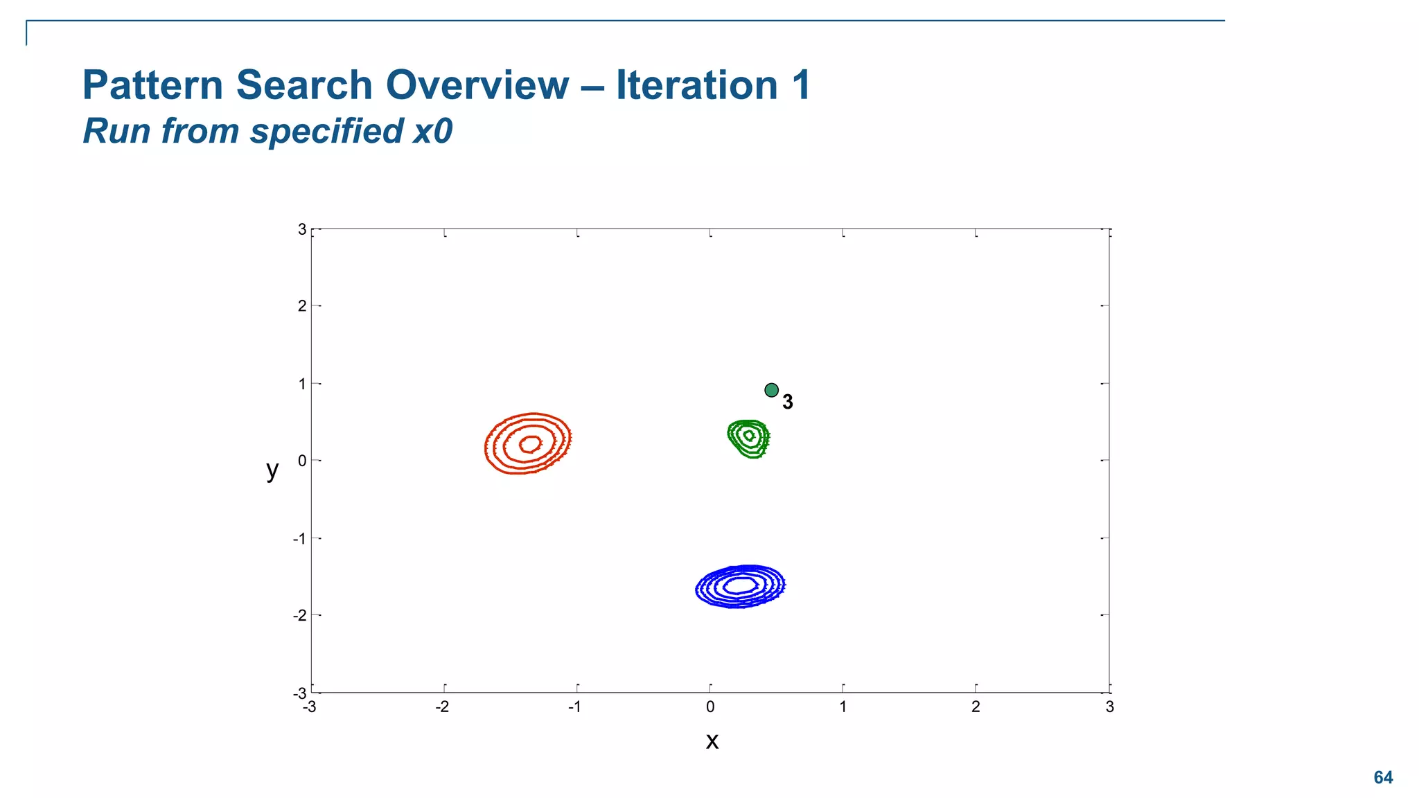
Pattern Search Overview – Iteration 1
Apply pattern vector, poll new points for improvement
x
y
3
Mesh size = 1
Pattern vectors = [1,0], [0,1], [-1,0], [0,-1]
0
_
*
_ x
vector
pattern
size
mesh
Pnew 

0
]
0
,
1
[
*
1 x


1.6
0.4
4.6
2.8
First poll successful
Complete Poll (not default)

68. 66
-3 -2 -1 0 1 2 3
-3
-2
-1
0
1
2
3
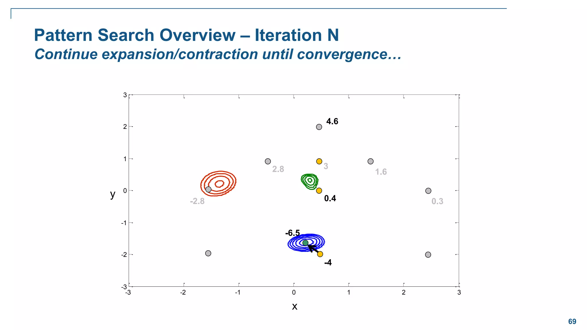
Pattern Search Overview – Iteration 2
x
y
3
Mesh size = 2
Pattern vectors = [1,0], [0,1], [-1,0], [0,-1]
1.6
0.4
4.6
2.8
-4
0.3
-2.8
Complete Poll

69. 67
-3 -2 -1 0 1 2 3
-3
-2
-1
0
1
2
3
Pattern Search Overview – Iteration 3
x
y
3
Mesh size = 4
Pattern vectors = [1,0], [0,1], [-1,0], [0,-1]
1.6
0.4
4.6
2.8
-4
0.3
-2.8

70. 68
-3 -2 -1 0 1 2 3
-3
-2
-1
0
1
2
3
Pattern Search Overview – Iteration 4
x
y
3
Mesh size = 4*0.5 = 2
Pattern vectors = [1,0], [0,1], [-1,0], [0,-1]
1.6
0.4
4.6
2.8
-4
0.3
-2.8

71. 69
-3 -2 -1 0 1 2 3
-3
-2
-1
0
1
2
3
Pattern Search Overview – Iteration N
Continue expansion/contraction until convergence…
x
y
3
1.6
0.4
4.6
2.8
-4
0.3
-2.8
-6.5

72. 70
Pattern Search – Peaks Function

73. 71
Pattern Search Climbs Mount Washington

74. 72
PARTICLE SWARM

75. 73
What is Particle Swarm Optimization?
 A collection of particles move
throughout the region
 Particles have velocity and are
affected by the other particles in
the swarm
 Does not rely on gradients: works
on smooth and nonsmooth
problems

76. 74
-3 -2 -1 0 1 2 3
-3
-2
-1
0
1
2
3
Particle Swarm Overview – Iteration 1
Initialize particle locations and velocities, evaluate all
locations
x
y

77. 75
-3 -2 -1 0 1 2 3
-3
-2
-1
0
1
2
3
Particle Swarm Overview – Iteration N
Update velocities for each particle
x
y
Previous
Velocity
Best Location
for this Particle
Best Location for
Neighbor Particles

78. 76
-3 -2 -1 0 1 2 3
-3
-2
-1
0
1
2
3
Particle Swarm Overview – Iteration N
Update velocities for each particle
x
y
New
Velocity

79. 77
-3 -2 -1 0 1 2 3
-3
-2
-1
0
1
2
3
Particle Swarm Overview – Iteration N
Move particles based on new velocities
x
y

80. 78
-3 -2 -1 0 1 2 3
-3
-2
-1
0
1
2
3
Particle Swarm Overview – Iteration N
Continue swarming until convergence
x
y

81. 79
Particle Swarm – Peaks Function

82. 80
GENETIC ALGORITHM

83. 81
What is a Genetic Algorithm?
 Uses concepts from evolutionary
biology
 Start with an initial generation of
candidate solutions that are tested
against the objective function
 Subsequent generations evolve
from the 1st through selection,
crossover and mutation

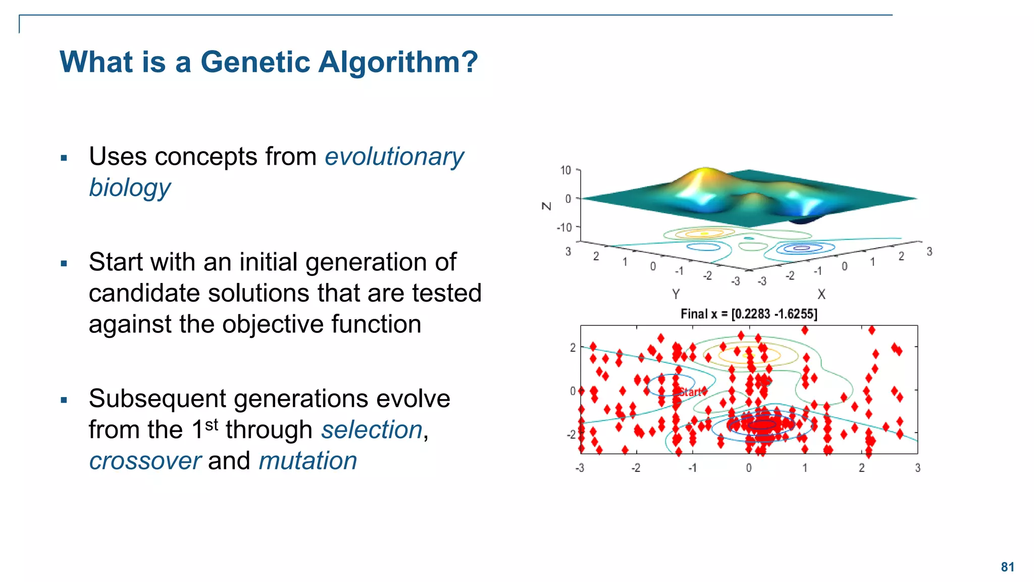
84. 82
How Evolution Works – Binary Case
 Selection
– Retain the best performing bit strings from one generation to the next. Favor these for
reproduction
– parent1 = [ 1 0 1 0 0 1 1 0 0 0 ]
– parent2 = [ 1 0 0 1 0 0 1 0 1 0 ]
 Crossover
– parent1 = [ 1 0 1 0 0 1 1 0 0 0 ]
– parent2 = [ 1 0 0 1 0 0 1 0 1 0 ]
– child = [ 1 0 0 0 0 1 1 0 1 0 ]
 Mutation
– parent = [ 1 0 1 0 0 1 1 0 0 0 ]
– child = [ 0 1 0 1 0 1 0 0 0 1 ]

85. 83
-3 -2 -1 0 1 2 3
-3
-2
-1
0
1
2
3
Genetic Algorithm – Iteration 1
Evaluate initial population
x
y

86. 84
-3 -2 -1 0 1 2 3
-3
-2
-1
0
1
2
3
Genetic Algorithm – Iteration 1
Select a few good solutions for reproduction
x
y

87. 85
-3 -2 -1 0 1 2 3
-3
-2
-1
0
1
2
3
Genetic Algorithm – Iteration 2
Generate new population and evaluate
x
y

88. 86
-3 -2 -1 0 1 2 3
-3
-2
-1
0
1
2
3
Genetic Algorithm – Iteration 2
x
y

89. 87
-3 -2 -1 0 1 2 3
-3
-2
-1
0
1
2
3
Genetic Algorithm – Iteration 3
x
y

90. 88
-3 -2 -1 0 1 2 3
-3
-2
-1
0
1
2
3
Genetic Algorithm – Iteration 3
x
y

91. 89
-3 -2 -1 0 1 2 3
-3
-2
-1
0
1
2
3
Genetic Algorithm – Iteration N
Continue process until stopping criteria are met
x
y
Solution found

92. 90
Genetic Algorithm – Peaks Function

93. 91
Genetic Algorithm – Integer Constraints
Mixed Integer Optimization
s.t. some x are integers
Examples
 Only certain sizes of components
available
 Can only purchase whole shares of stock
)
(
min x
f
x

94. 92
Application: Circuit Component Selection
 6 components to size
 Only certain sizes available
 Objective:
– Match Voltage vs. Temperature
curve
Thermistor Circuit
300 Ω
330 Ω
360 Ω
…
180k Ω
200k Ω
220k Ω
Thermistors:
Resistance varies
nonlinearly with
temperature
?
𝑅𝑇𝐻 =
𝑅𝑇𝐻,𝑁𝑜𝑚
𝑒
𝛽
𝑇−𝑇𝑁𝑜𝑚
𝑇∗𝑇𝑁𝑜𝑚

95. 93
Global Optimization Toolbox Solvers
 GlobalSearch, MultiStart
– Well suited for smooth objective and constraints
– Return the location of local and global minima
 ga, gamultiobj, simulannealbnd, particleswarm
– Many function evaluations to sample the search space
– Work on both smooth and nonsmooth problems
 patternsearch
– Fewer function evaluations than ga, simulannealbnd, particlewarm
– Does not rely on gradient calculation like GlobalSearch and MultiStart
– Works on both smooth and nonsmooth problems

96. 94
Optimization Toolbox Solvers
 fmincon, fminbnd, fminunc, fgoalattain, fminimax
– Nonlinear constraints and objectives
– Gradient-based methods for smooth objectives and constraints
 quadprog, linprog
– Linear constraints and quadratic or linear objective, respectively
 intlinprog
– Linear constraints and objective and integer variables
 lsqlin, lsqnonneg
– Constrained linear least squares
 lsqnonlin, lsqcurvefit
– Nonlinear least squares
 fsolve
– Nonlinear equations

97. 95
Speeding-up with Parallel Computing
 Global Optimization solvers that support Parallel
Computing:
– ga, gamultiobj: Members of population evaluated in parallel
at each iteration
– patternsearch: Poll points evaluated in parallel at each
iteration
– particleswarm: Population evaluated in parallel at each
iteration
– MultiStart: Start points evaluated in parallel
 Optimization solvers that support Parallel Computing:
– fmincon: parallel evaluation of objective function for finite
differences
– fminunc, fminimax, fgoalattain,fsolve,
lsqcurvefit, lsqnonlin: same as fmincon
 Parallel Computing can also be used in the Objective
Function
– parfor

98. 96
 Speed up parallel applications
 Take advantage of GPUs
 Prototype code for your cluster
Parallel Computing Toolbox for the Desktop
Simulink, Blocksets,
and Other Toolboxes
Local
Desktop Computer
MATLAB
…
…

99. 97
Scale Up to Clusters and Clouds
Cluster
Scheduler
Computer Cluster
…
…
…
…
…
…
…
…
…
Simulink, Blocksets,
and Other Toolboxes
Local
Desktop Computer
MATLAB
…
…

100. 98
Learn More about Optimization with MATLAB
Recorded webinar: Optimization in
MATLAB: An Introduction to Quadratic
Programming
Optimization Toolbox Web demo:
Finding an Optimal Path using MATLAB
and Optimization Toolbox
MATLAB Digest: Improving
Optimization Performance with Parallel
Computing
MATLAB Digest: Using Symbolic
Gradients for Optimization
Recorded webinar: Mixed Integer
Linear Programming in MATLAB
Recorded webinar: Optimization in
MATLAB for Financial Applications
1 2 3 4 5
0
500
1000
1500
2000
2500
3000
Bonds
#
Purchased
Cash Flow Matching Example

101. 99
Key Takeaways
 Solve a wide variety of optimization problems in MATLAB
– Linear and Nonlinear
– Continuous and mixed-integer
– Smooth and Nonsmooth
 Find better solutions to multiple minima and non-smooth problems using global
optimization
 Use symbolic math for setting up problems and automatically calculating gradients
 Using parallel computing to speed up optimization problems

102. Questions?