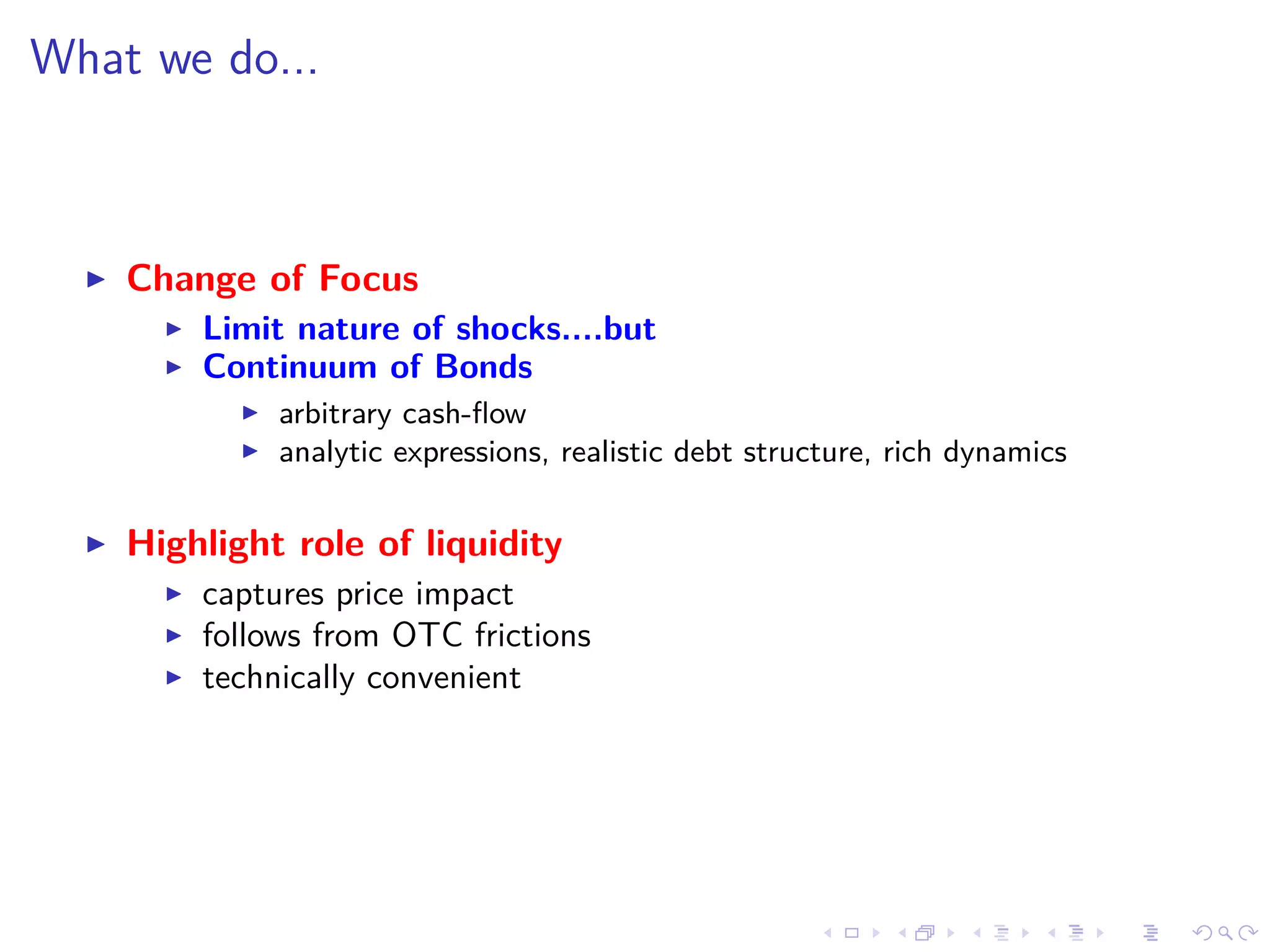
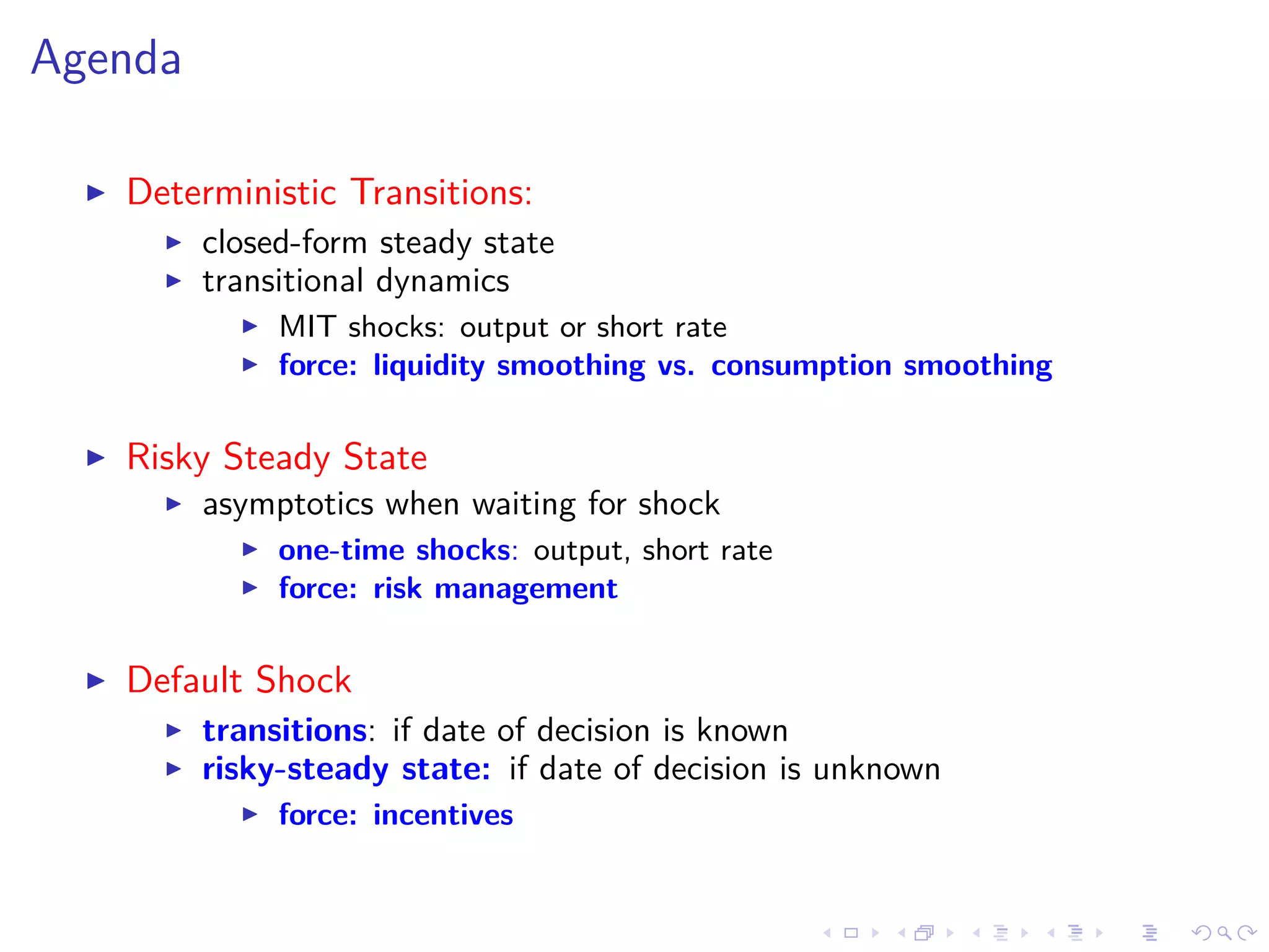
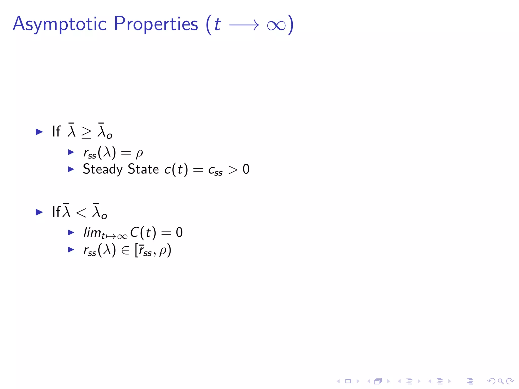
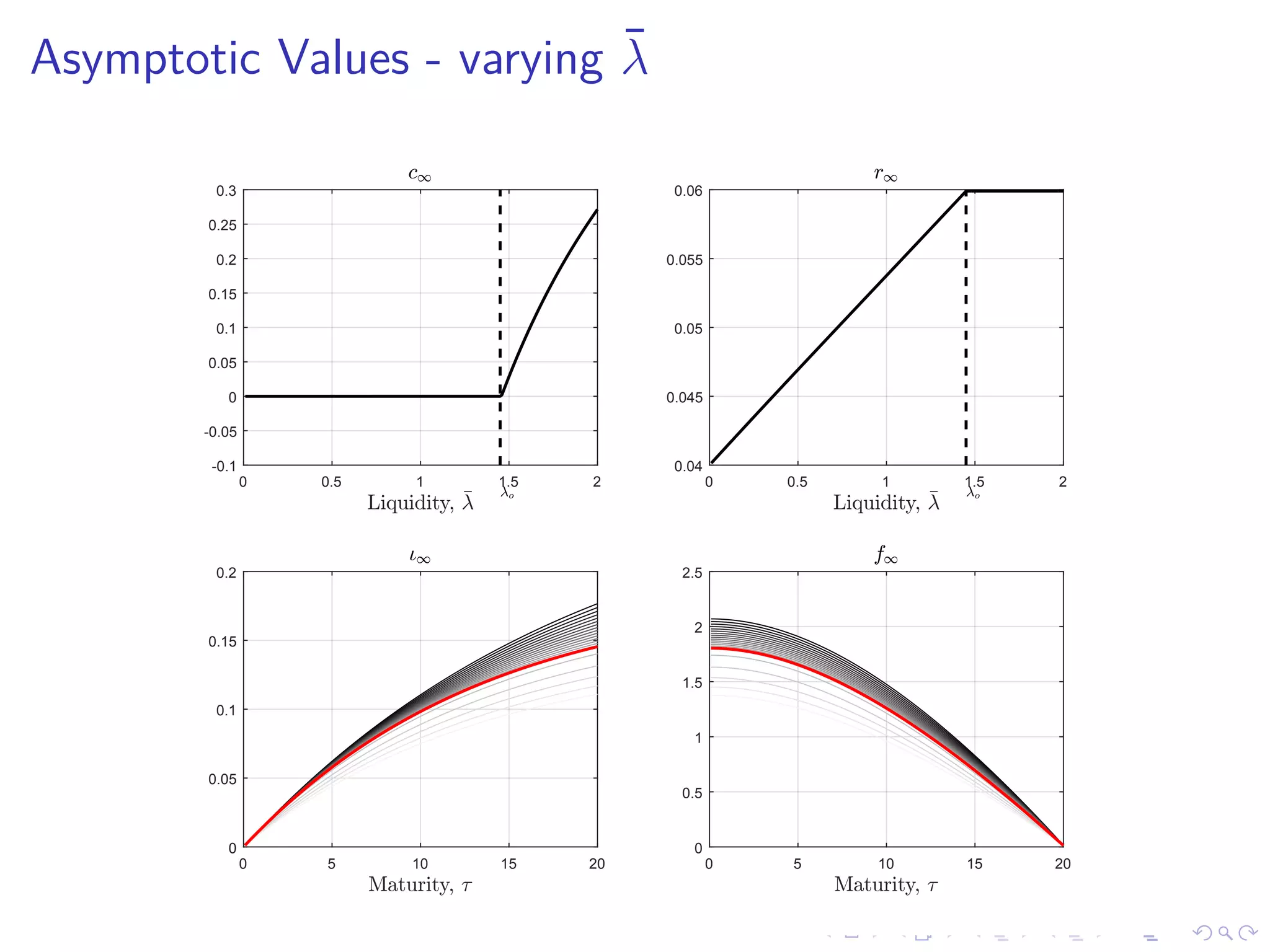
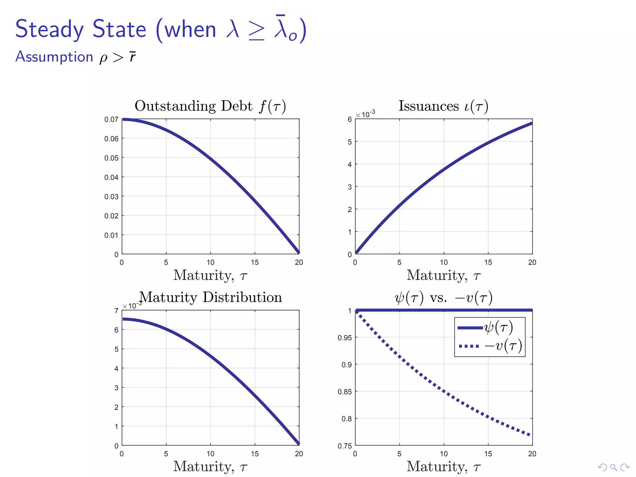
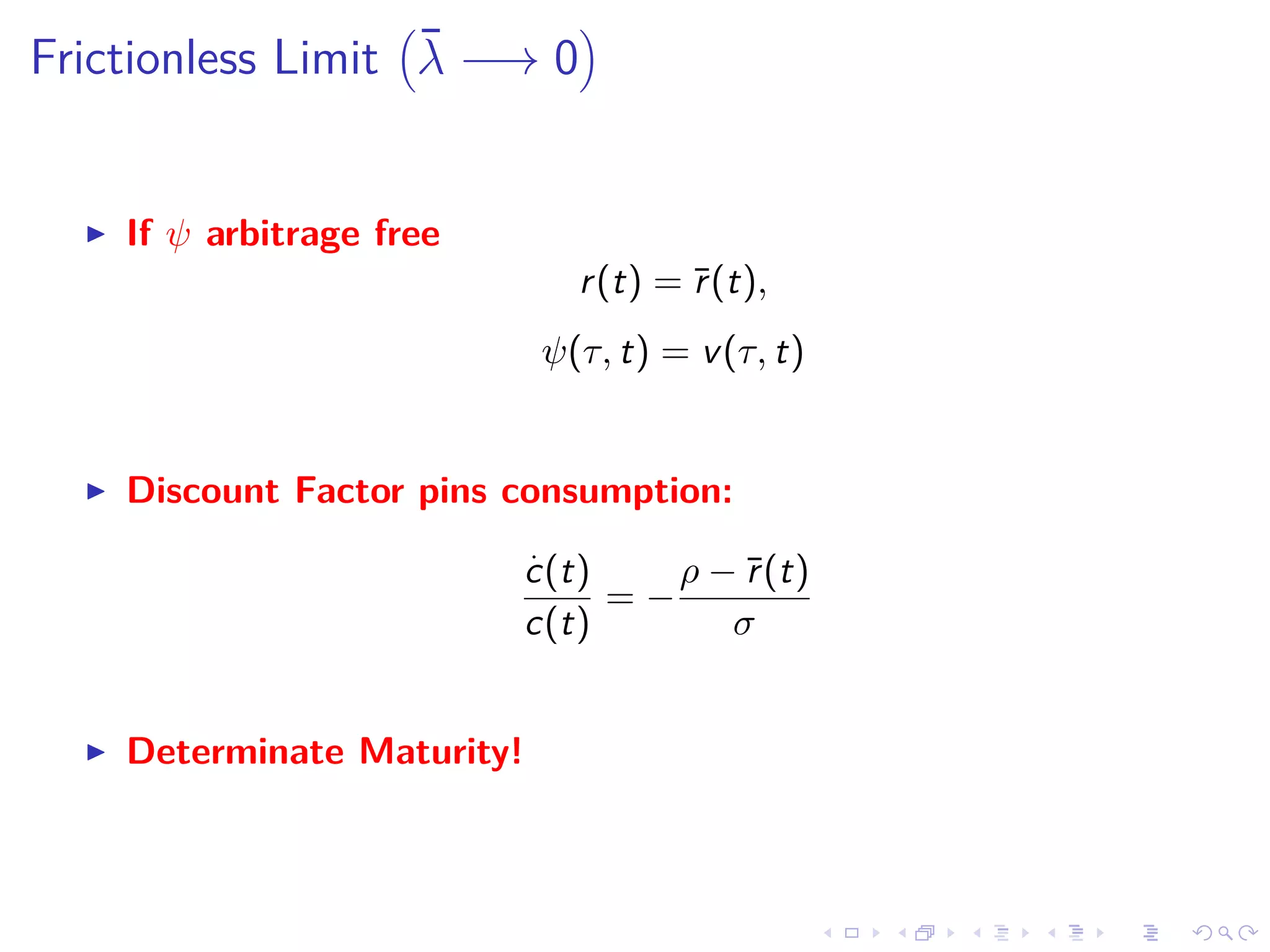
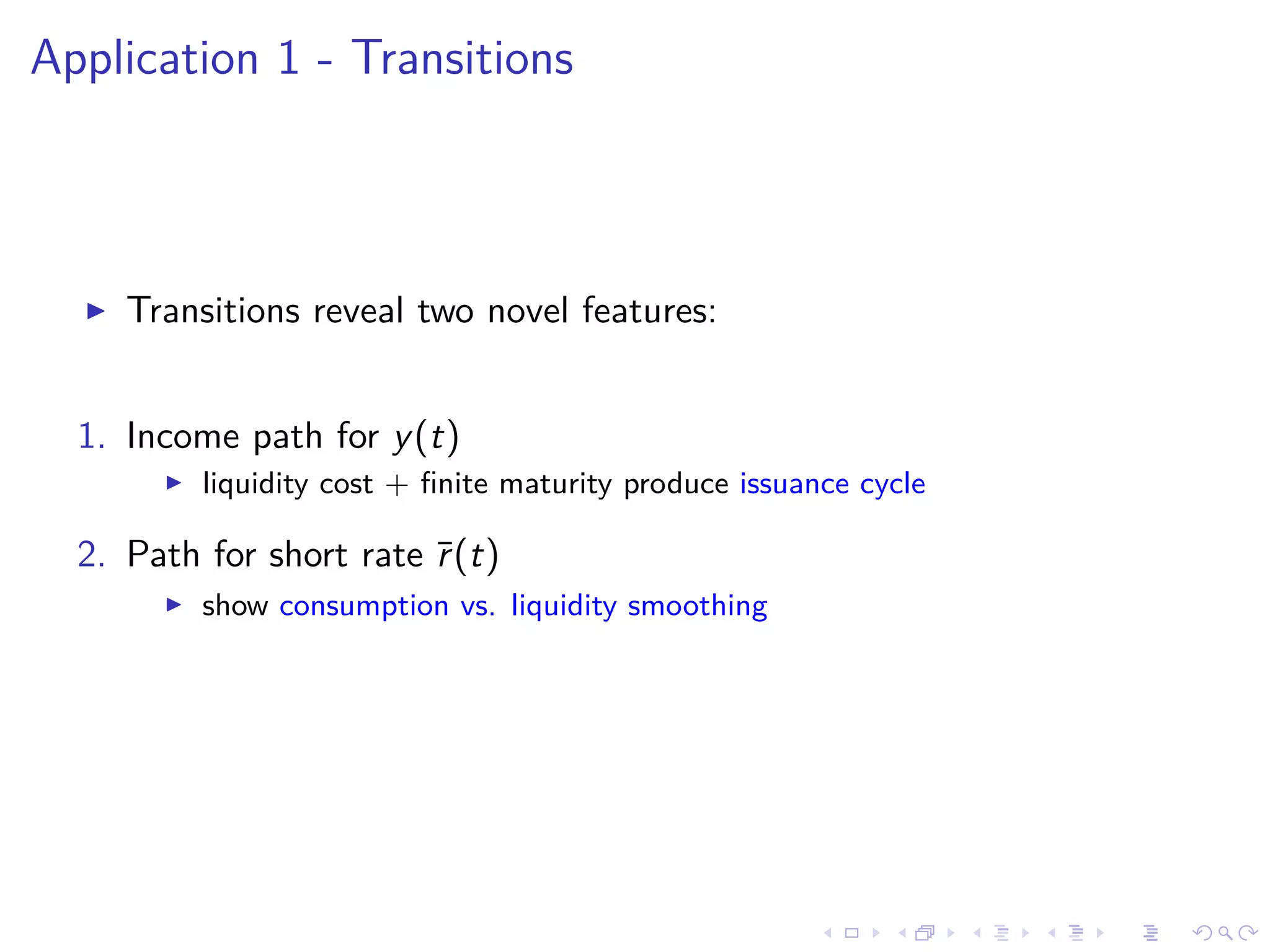
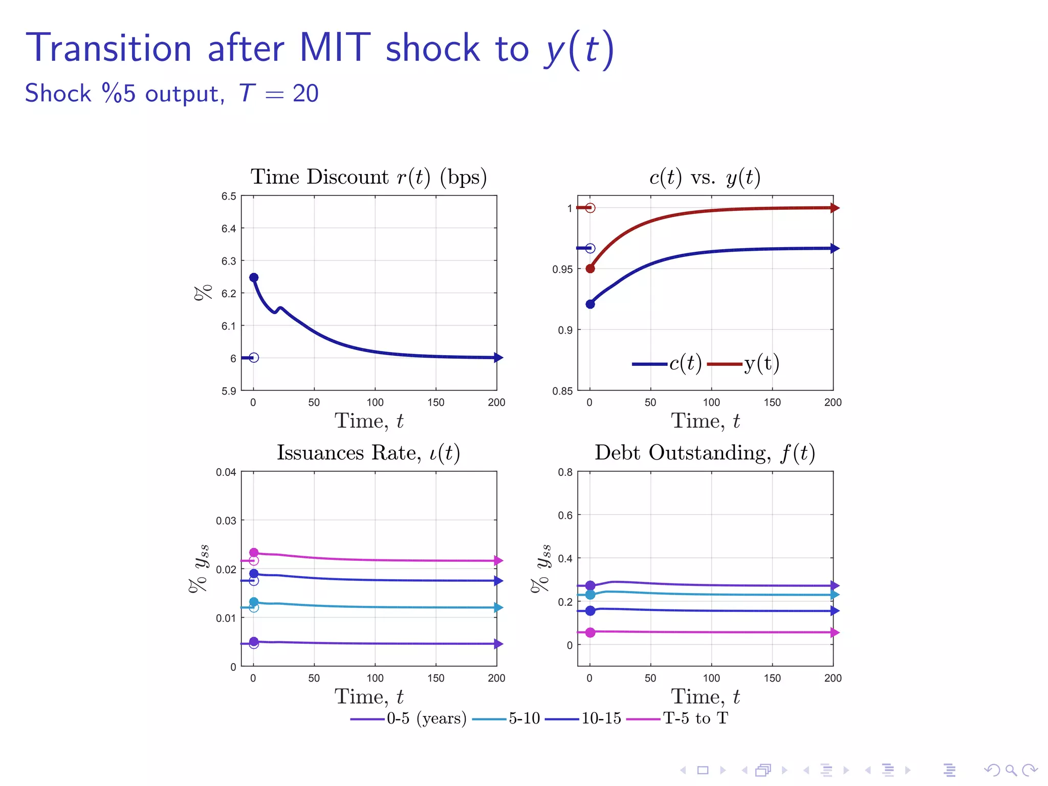
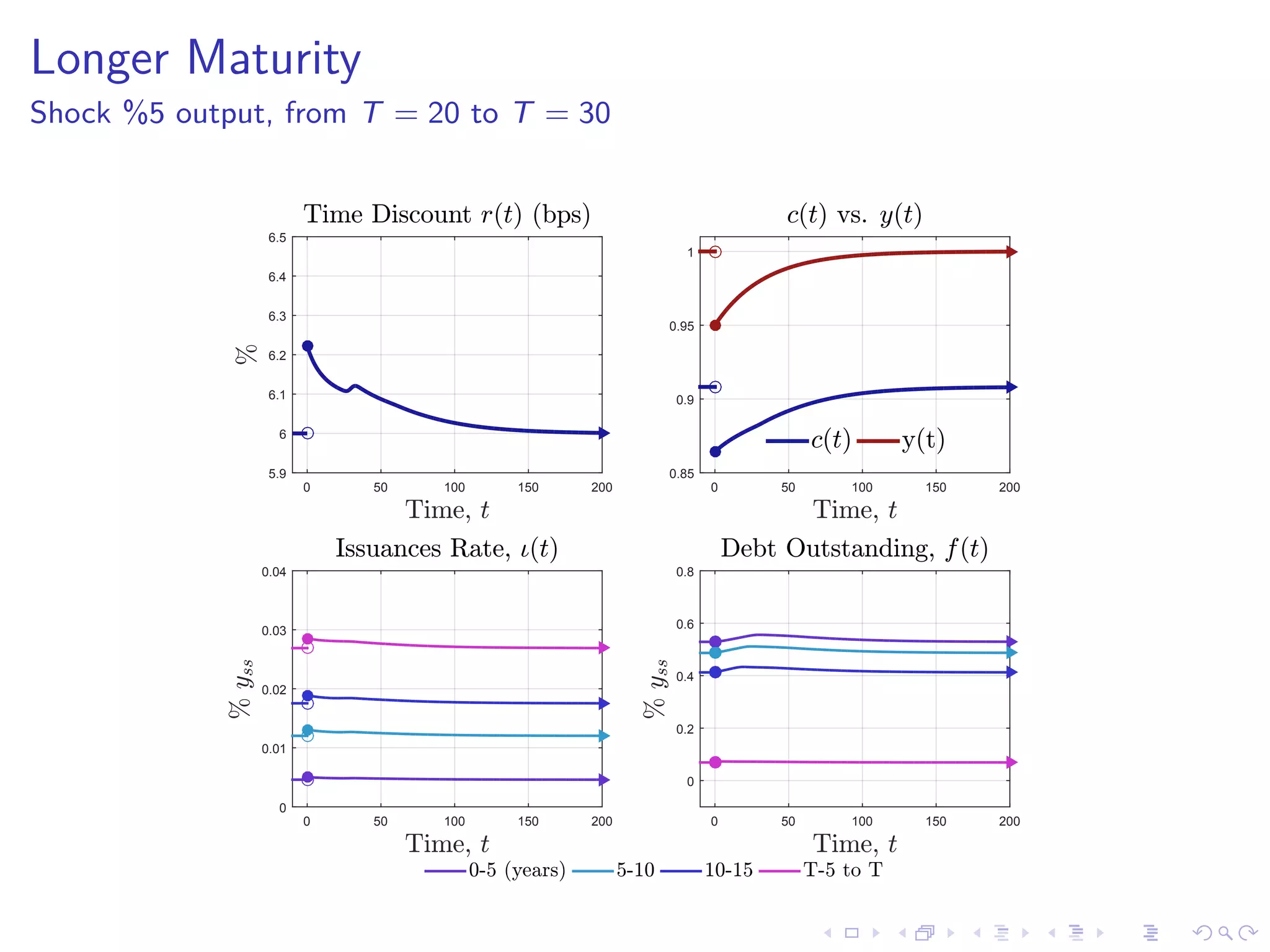
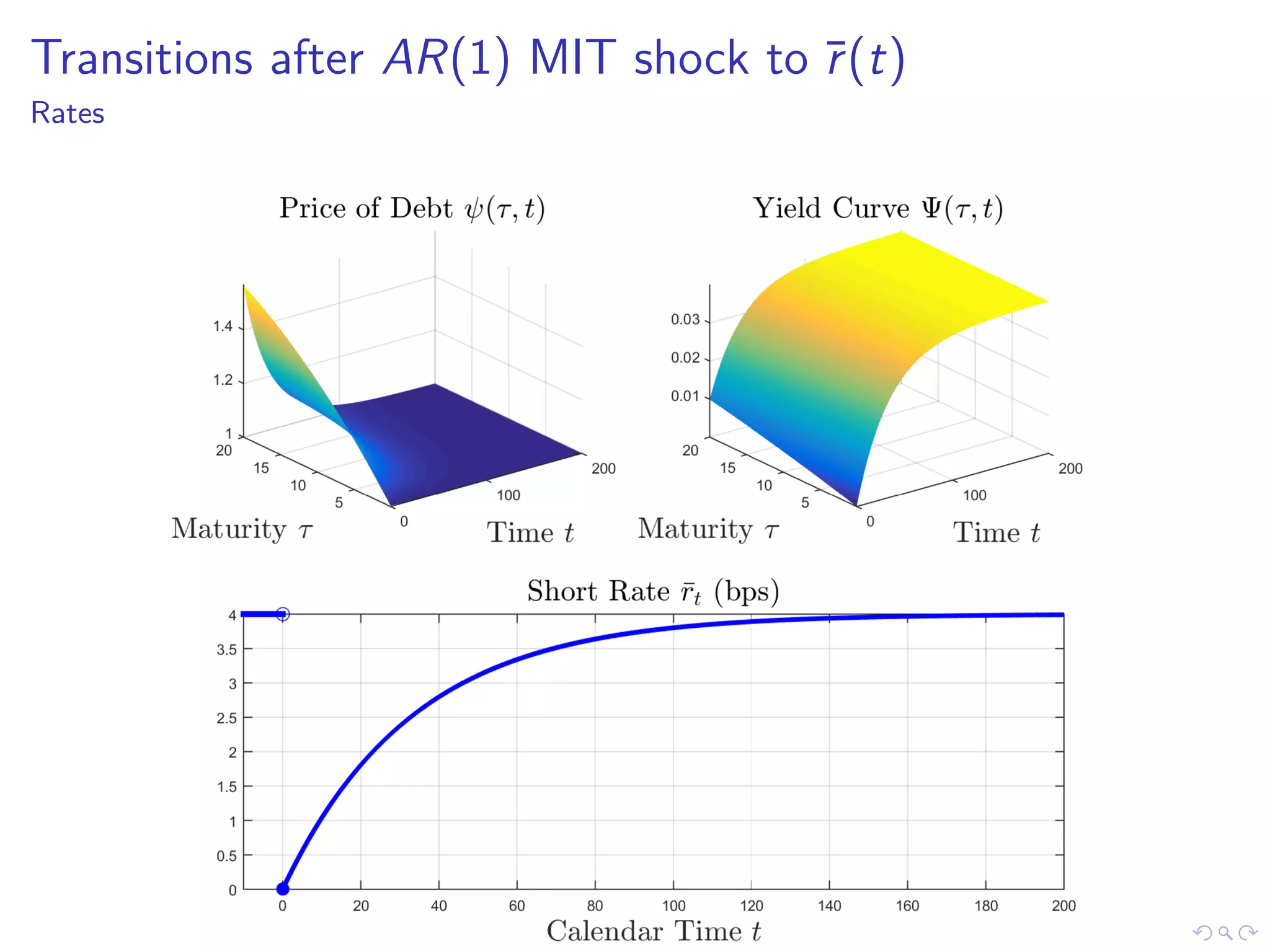
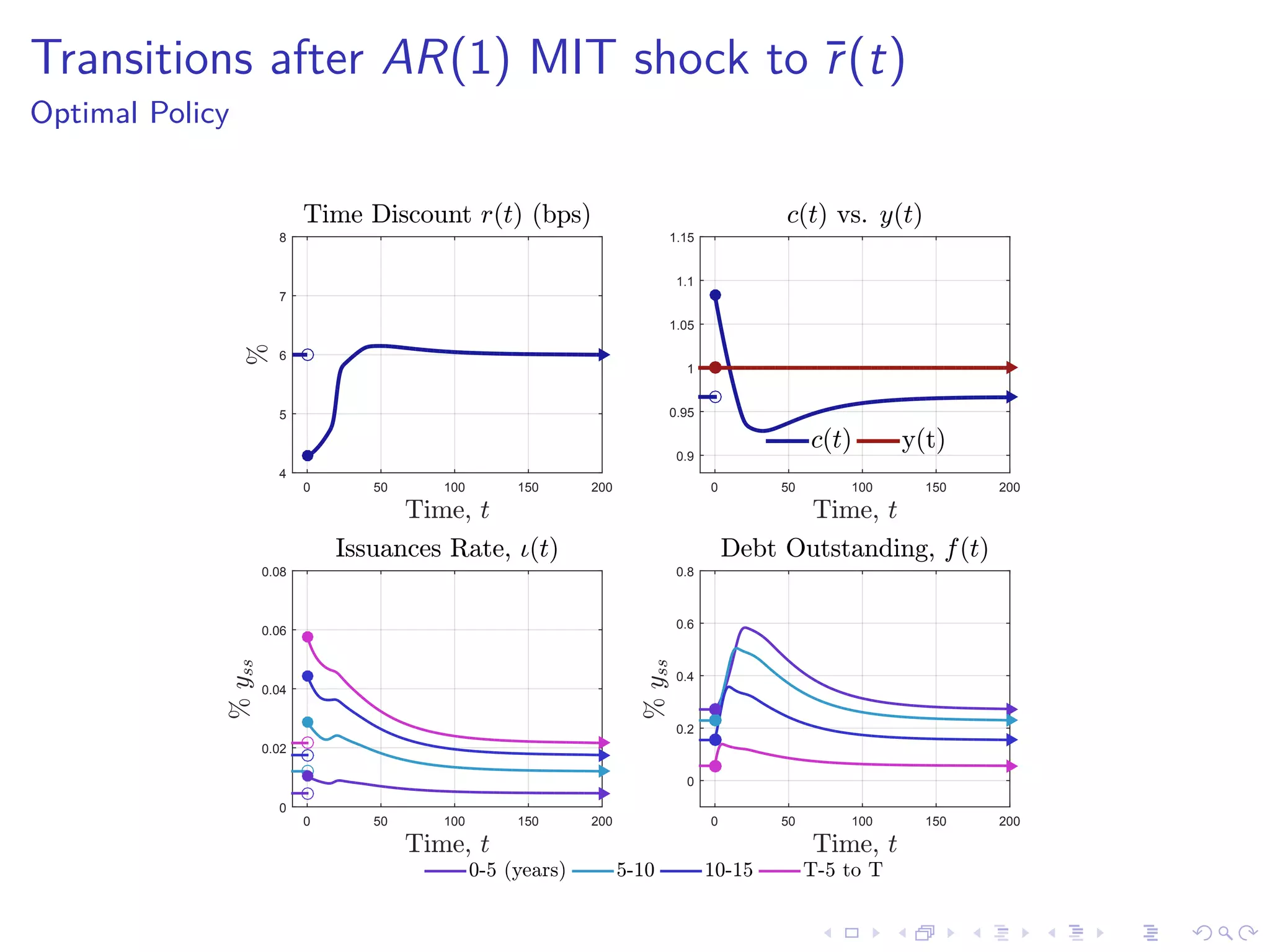
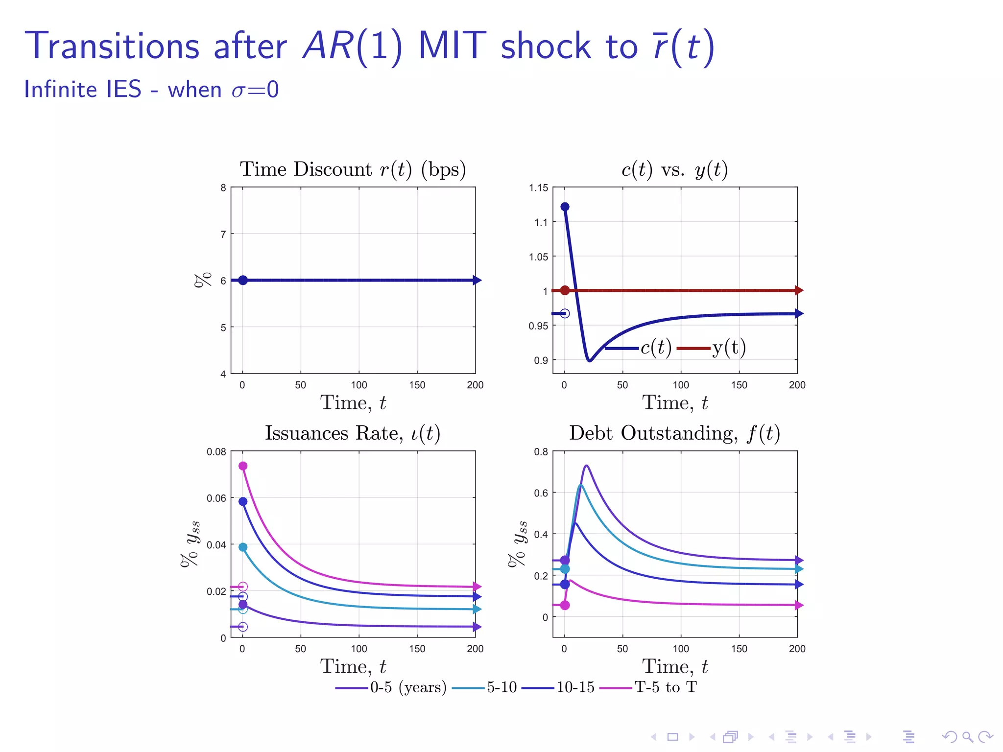
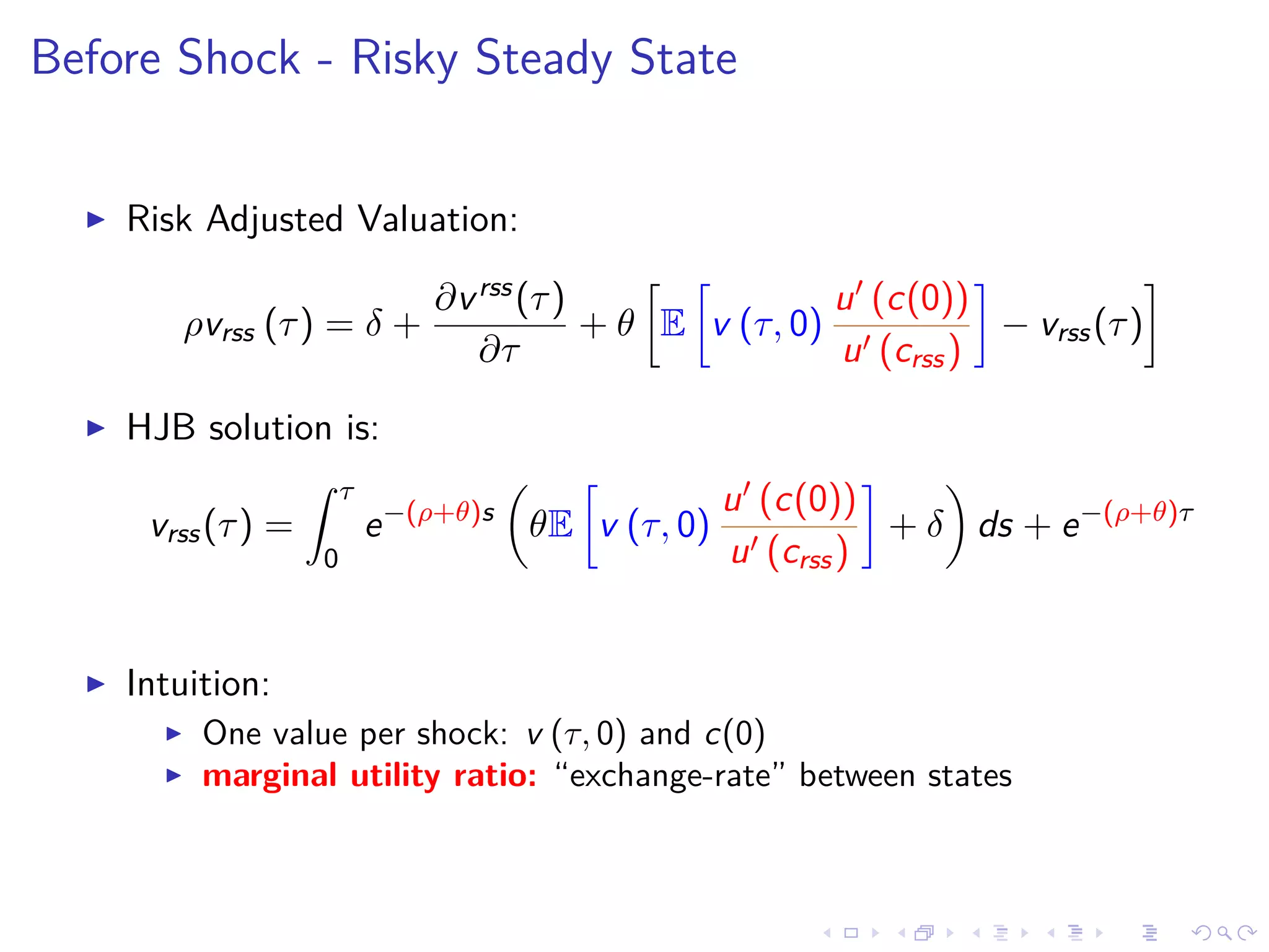
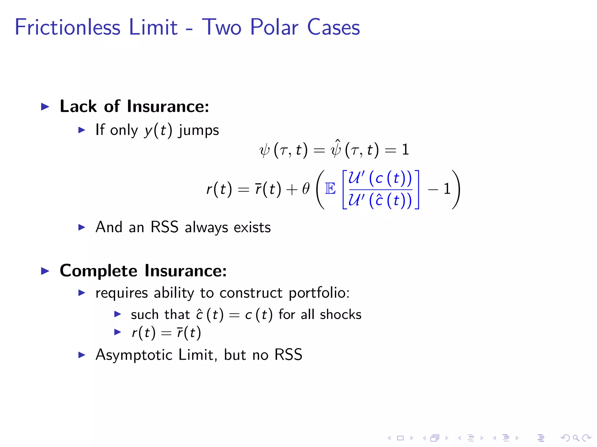
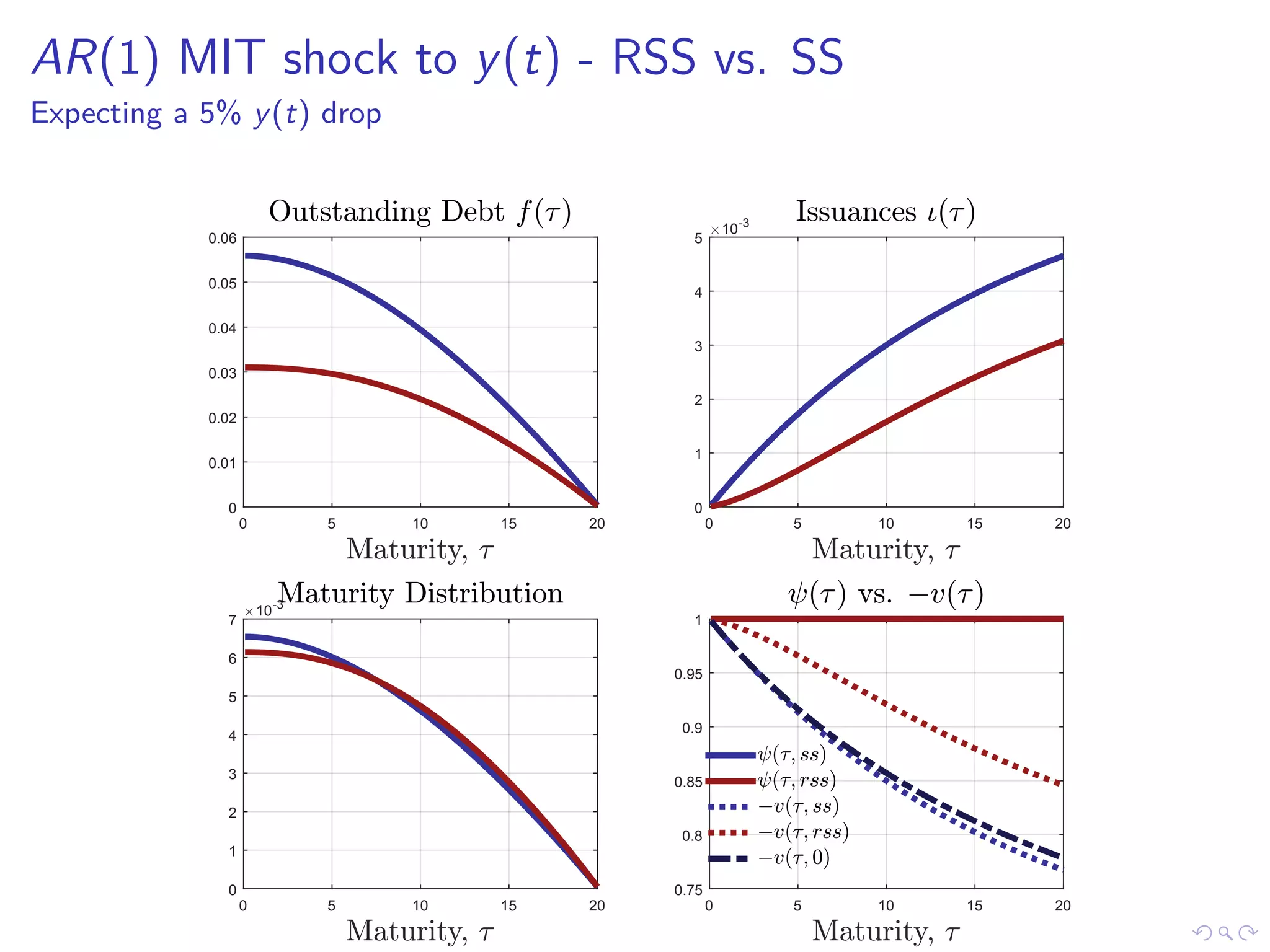
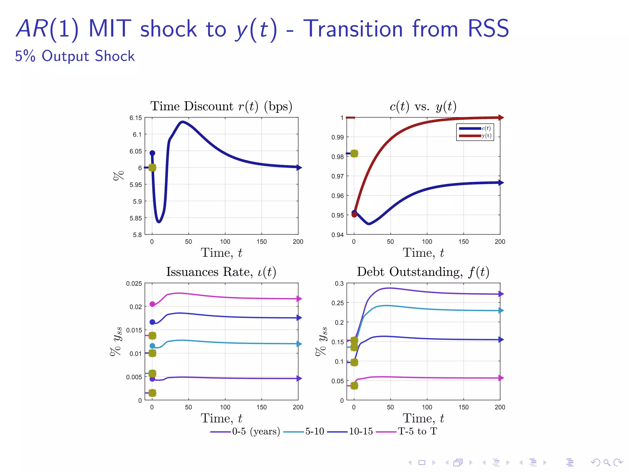
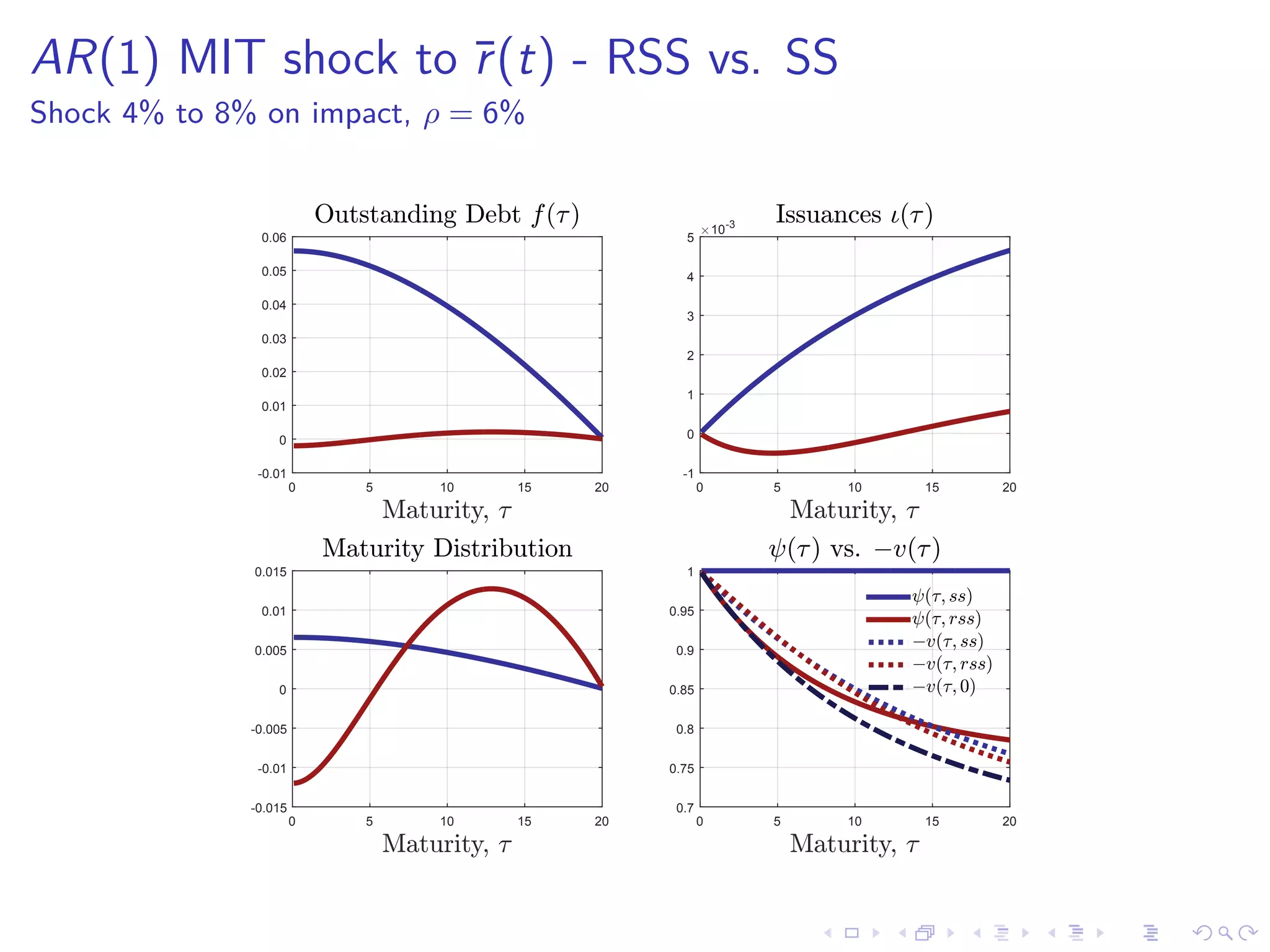
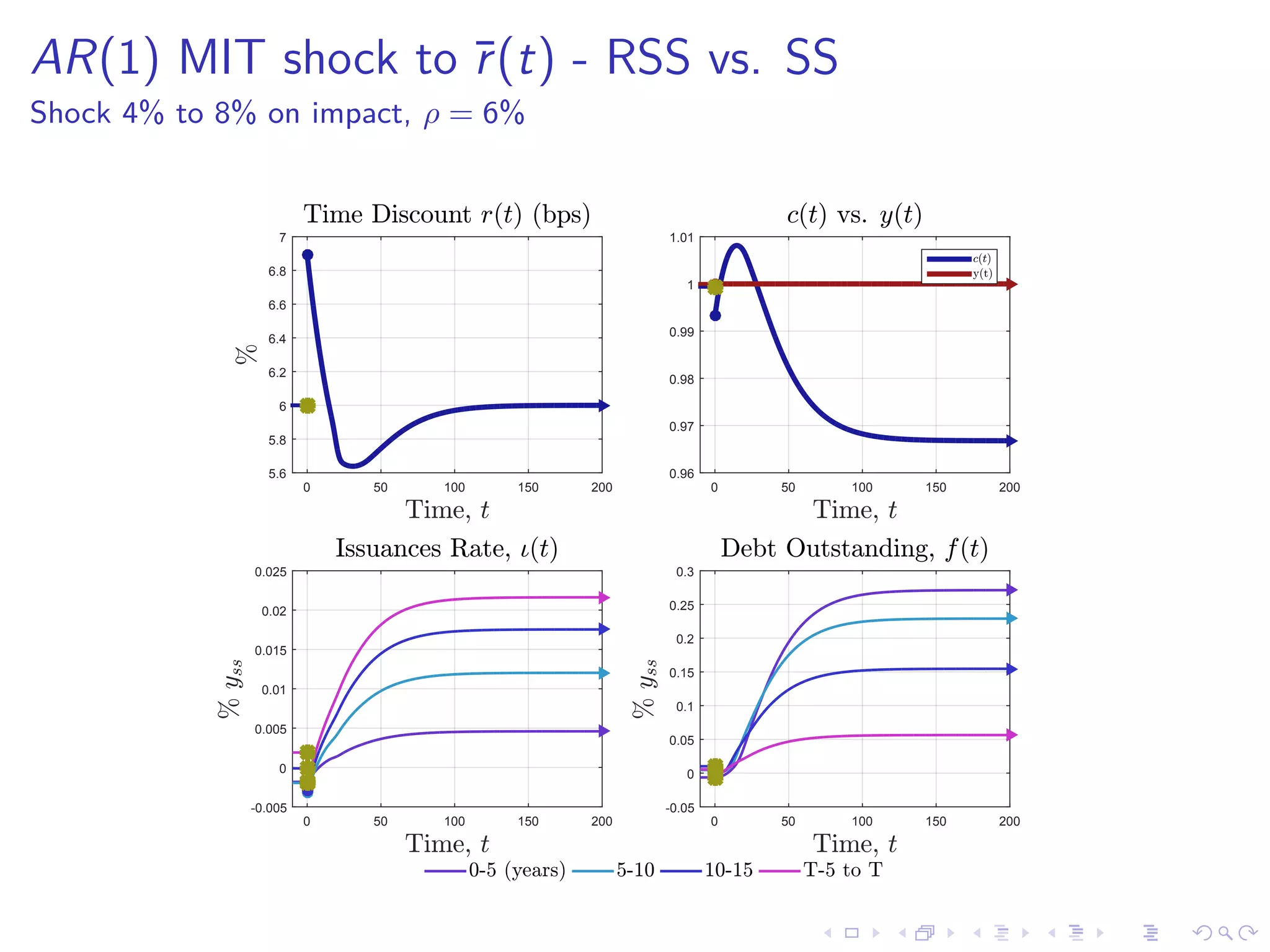
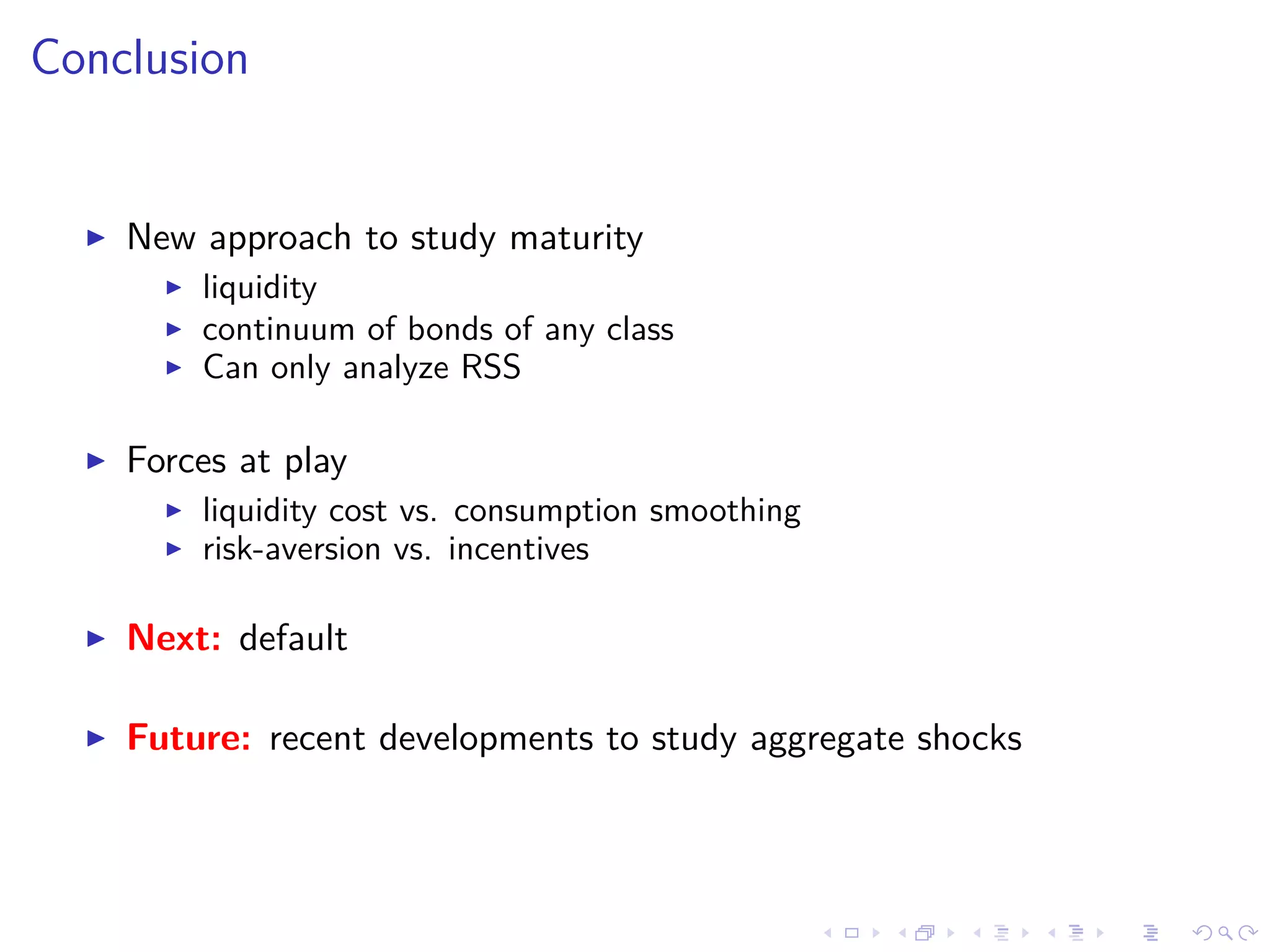
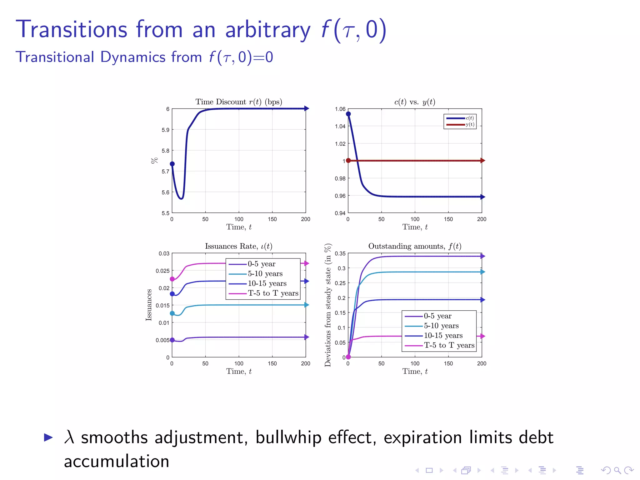
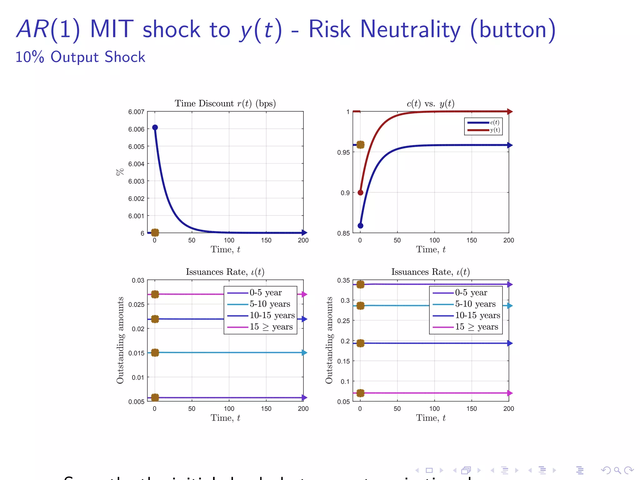
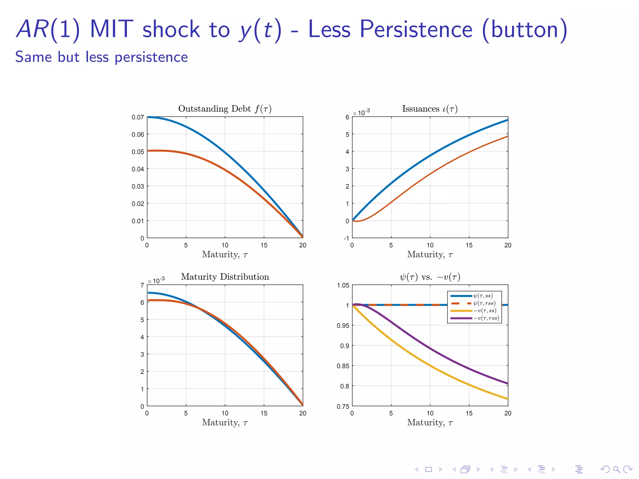
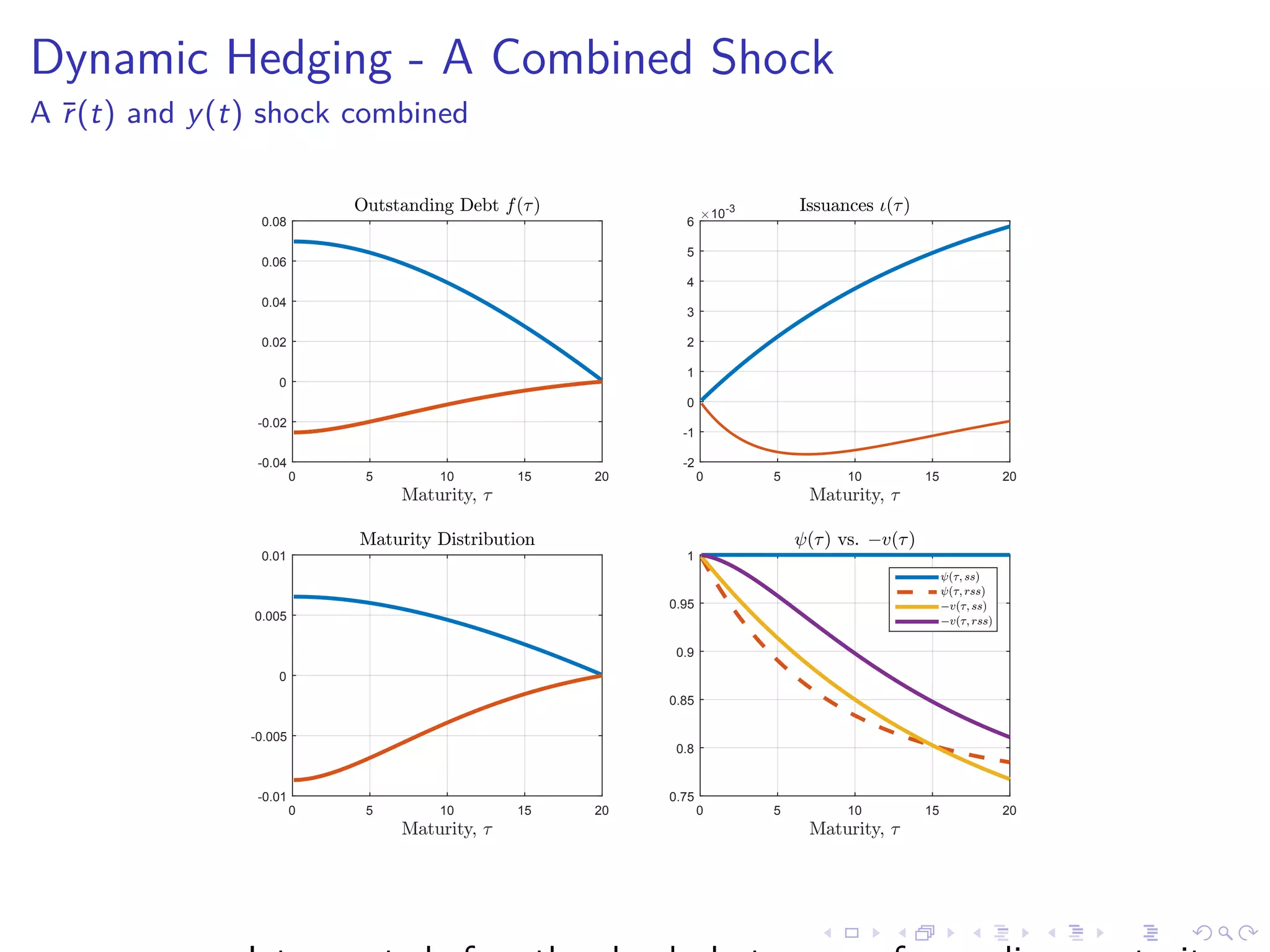
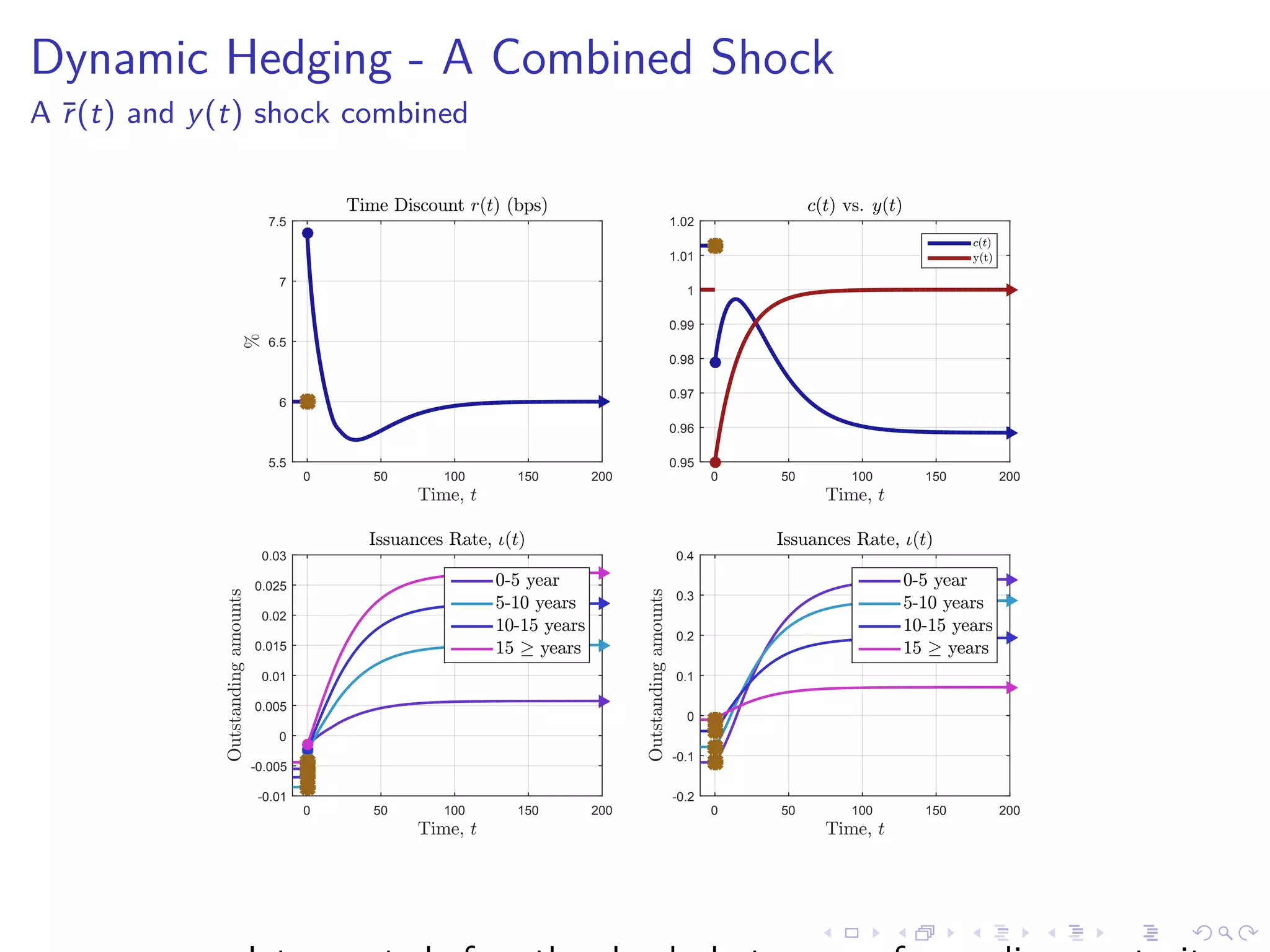
This document discusses optimal debt maturity management. It presents a model where a sovereign can issue a continuum of bonds with arbitrary cash flows to examine debt dynamics. The model highlights the role of liquidity costs in shaping issuance and maturity choices. It shows that income and interest rate shocks can lead to cycles in issuance as the sovereign balances liquidity smoothing versus consumption smoothing. Longer maturity horizons and interest rate shocks emphasize consumption smoothing over liquidity smoothing in transitions following shocks.

1. Optimal Debt-Maturity Management
Saki Bigio (UCLA)
Galo Nuño (Bank of Spain)
Juan Passadore (EIEF)
Toulouse, April 2018

2. Peru Example - Programmed Coupon Payments
Number of years in the future
5 10 15 20 25 30 35
%ofAnnualGDP
0
0.05
0.1
0.15
0.2
0.25
0.3
0.35
0.4
0.45
0.5
Interests-2016 Q2

3. Peru Example - Programmed Principal Payments
Number of years in the future
5 10 15 20 25 30 35
%ofAnnualGDP
0
0.1
0.2
0.3
0.4
0.5
0.6
0.7
Amortization-2016 Q2

4. Debt-Management
Large-Stake but highly complex problem
state-space: vector of bonds of different maturity
risks: income, interest-rate, default
forces: smoothing, risk management, incentives, liquidity
State of the art economics
Can handle many risks
Challenge:
use standard bond =⇒ ↑curse of dimensionality
forces use of consols
typically two

5. What we do...
Change of Focus
Limit nature of shocks....but
Continuum of Bonds
arbitrary cash-flow
analytic expressions, realistic debt structure, rich dynamics
Highlight role of liquidity
captures price impact
follows from OTC frictions
technically convenient

6. Environment
SOE, CT, incomplete markets, exogenous short rates
CT: elegance, speed and comp stats
Consumption-Savings Problem:
shocks: income, short rates, default value
liquidity cost
State Variable:
mass of debt/assets f (τ, t)

7. Agenda
Deterministic Transitions:
closed-form steady state
transitional dynamics
MIT shocks: output or short rate
force: liquidity smoothing vs. consumption smoothing
Risky Steady State
asymptotics when waiting for shock
one-time shocks: output, short rate
force: risk management
Default Shock
transitions: if date of decision is known
risky-steady state: if date of decision is unknown
force: incentives

8. Literature
Sovereign Debt: Eaton Gersovitz (1981), Bulow Rogoff (1988), Arellano
(2008), Chattarjee Eiyungor (2012), Arellano Ramayanan (2012), Bianchi
Hatchondo Martinez (2014), Debortoli, Nunes, Yared (2017), Fernández
Martin (2014), Aguiar Amador Hopenhayn Werning (2017)
Preferred Habit Models: Modigliani and Stutch (1966), Greenwood
Vayanos (2010), Vayanos and Vila (2010)
Debt Management w/ Distortionary Taxes: Lucas Stokey (1983),
Angeletos (2002), Buera Nicolini (2004), Bhandari Evans Golosov Sargent
(2017)
Continuous Time - Heterogeneous Agents: Kredler (2014), Nuno Moll
(2017), Nuno Thomas (2017),

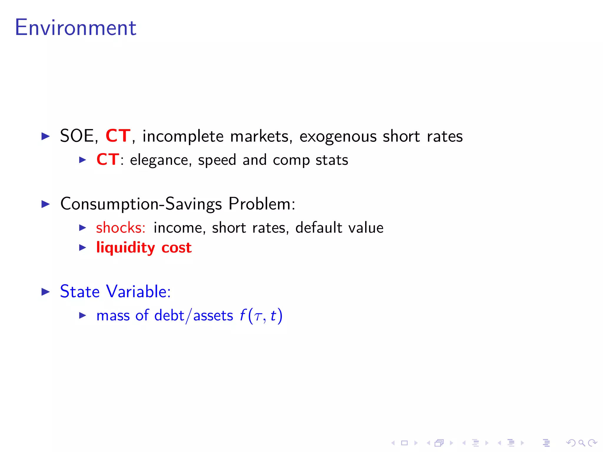
9. Environment: shocks, preference and state
Random paths: income y(t), short rate ¯r(t)
later: default
Preferences:
V0 = E[
∞
0
e−ρt
u(c(t))dt] and u(x) ≡
c1−σ − 1
1 − σ
State: debt f (τ, t), expiration τ ∈ [0, T]

10. Environment: constraint set
Resource Constraint:
c (t) = y (t) +
T
0
q (τ, t, ι) ι (τ, t)dτ
issuance
− f (0, t)
principal
−δ
T
0
f (τ, t) dτ
coupons
.
Bond price:
q (τ, t, ι) = ψ(τ, t)
bond price
−
1
2
ψ(τ, t)λ(ι)
liquidity cost
PDE constraint: Derivation
∂f (τ, t)
∂t
= ι (τ, t) +
∂f (τ, t)
∂τ
; f (τ, 0) = f0(τ)

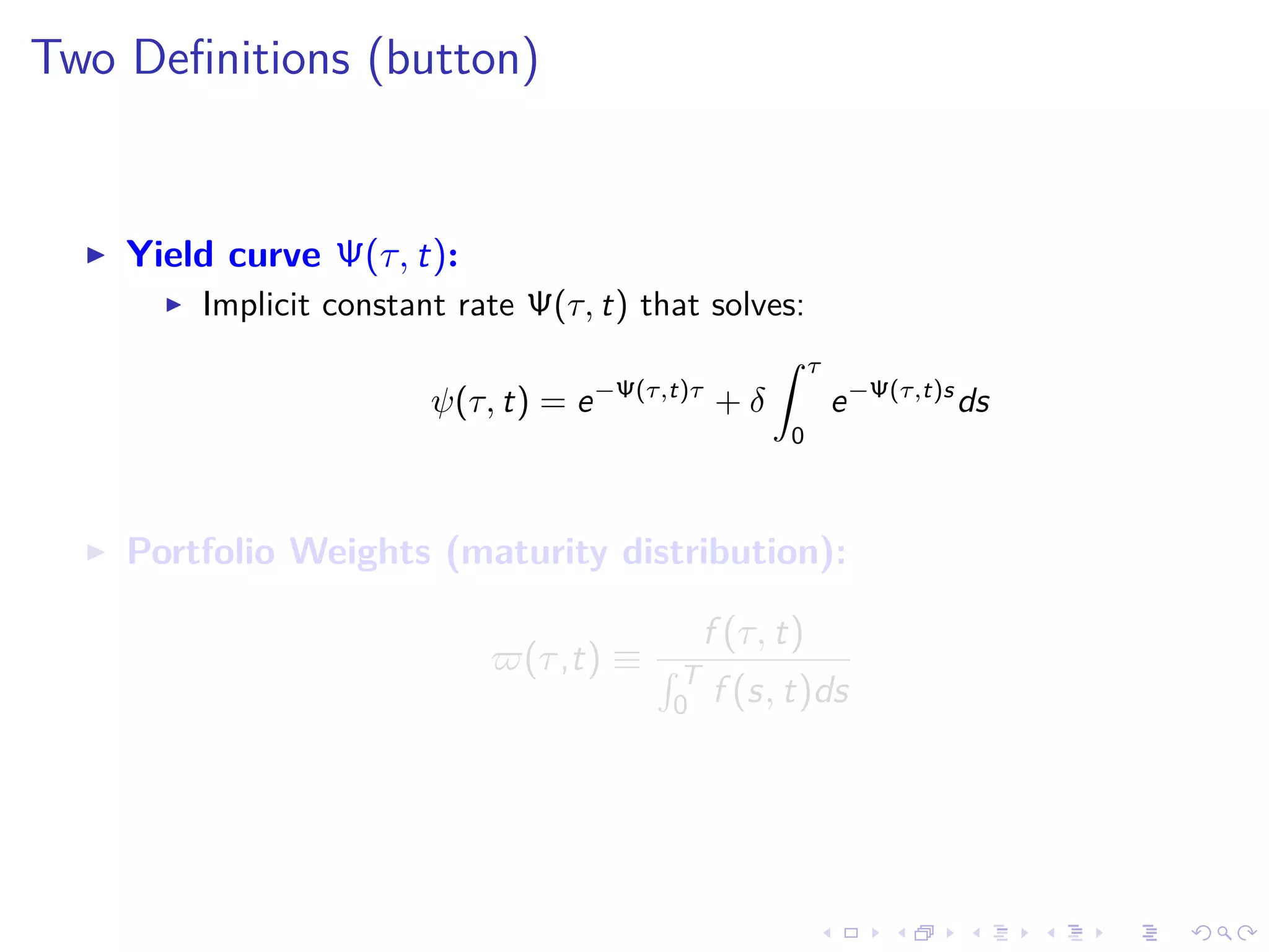
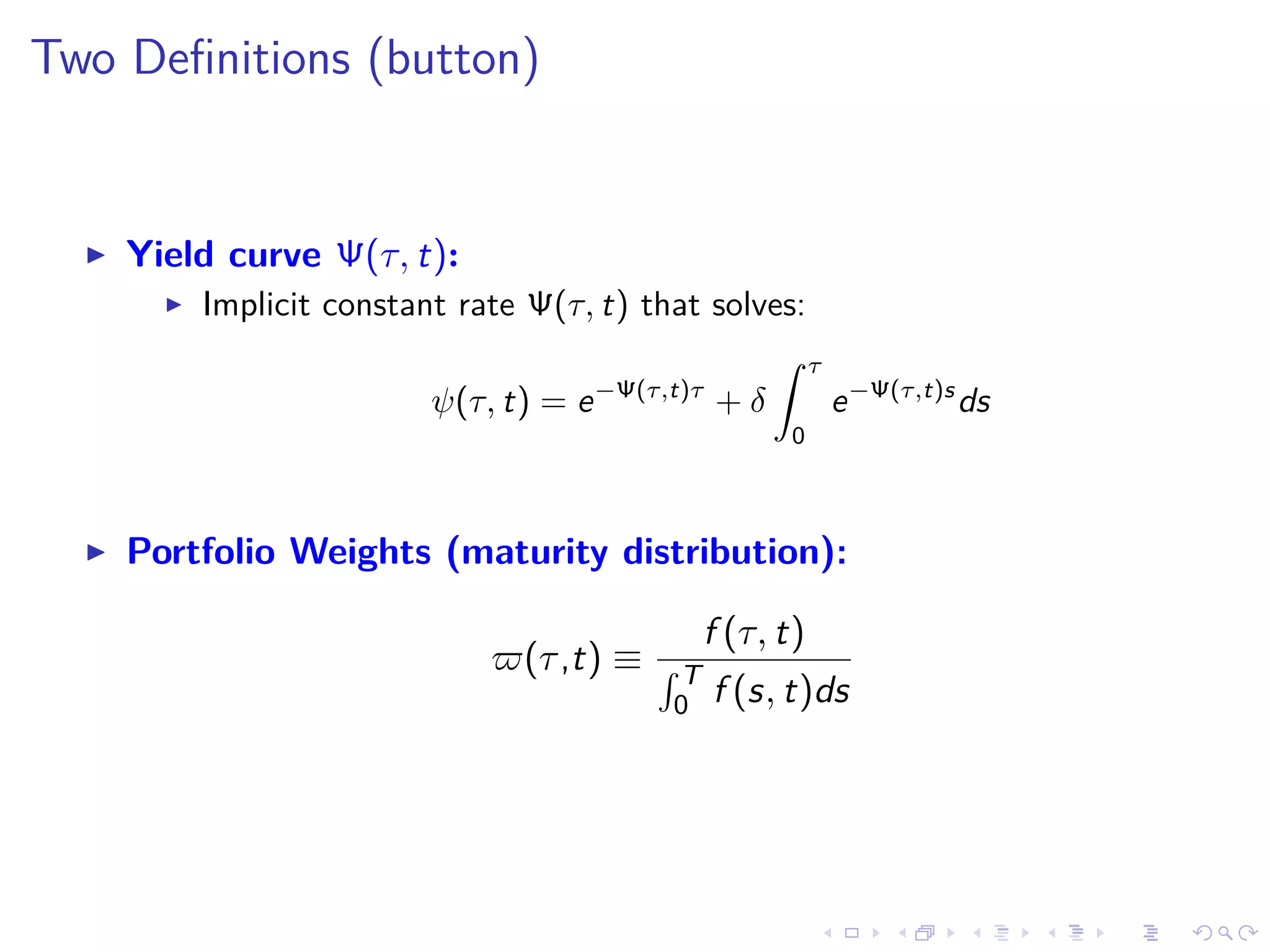
11. Environment: bond price
Bond Price ψ(τ, t):
short rate ¯r(t) path and no-arbitrage:
ψ(τ, t) = E[e
−
τ
0
¯r(t+s)ds
+ δ
τ
0
e
−
s
0
¯r(t+z)dz
ds]
In HJB form:
¯r(t)ψ(τ, t) = δ +
∂ψ
∂t
−
∂ψ
∂τ
; ψ(0, t) = 1

12. Environment: liquidity cost
WholesaleRetail bond market
Walrasian wholesale auction of ι (τ, t)
investment banks only
price cash-flow at ¯r (t) + η
OTC retail market
µ flow of clients match with banks
client valuation ψ(τ, t)
Auction price:
q(τ, t, ι) ψ(τ, t) −
1
2
ψ(τ, t) ¯λι
λ(ι)
,
and
¯λ ≡
η
µyss
.

13. General Problem
Perfect Foresight
V [f (·, 0)] = max
{ι(τ,t)}t∈[0,∞),τ∈[0,T]
Et
∞
t
e−ρ(s−t)
u(c(s))ds s.t.
c (t) = y (t) − f (0, t) +
T
0
[q (τ, t, ι) ι (τ, t) − δf (τ, t)] dτ
∂f
∂t
= ι (τ, t) +
∂f
∂τ
; f (τ, 0) = f0(τ)
Dual: Dual

14. Deterministic Dynamics
Theory

15. Deterministic Paths
no default, known paths, f0 given
Next...
derive steady-state distribution f ∗(τ)
path for transitional dynamics: f0 → f ∗(τ)
comparative statistics: f ∗(τ, X) → f ∗(τ, X )

16. Solving it
Step 1. Lagrangian
L (ι, f ) =
∞
0
e−ρt
u (c(t)) dt
+
∞
0
T
0
e−ρt
j (τ, t) −
∂f
∂t
+ ι (τ, t) +
∂f
∂τ
dτdt,
c(t) = y (t) − f (0, t) +
T
0
[q (t, τ, ι) ι (τ, t) − δf (τ, t)] dτ.
Step 2. First-Order Condition and Envelope
Marginal Value
u (c) q (τ, t, ι) +
∂q
∂ι
ι (τ, t) =
Marginal Cost
−j (τ, t)
ρj (τ, t) = −δu (c (t)) +
∂j
∂t
−
∂j
∂τ
, if τ ∈ (0, T]
and j (0, t) = −u (c (t)) .

17. Solving it
Step 1. Lagrangian
L (ι, f ) =
∞
0
e−ρt
u (c(t)) dt
+
∞
0
T
0
e−ρt
j (τ, t) −
∂f
∂t
+ ι (τ, t) +
∂f
∂τ
dτdt,
c(t) = y (t) − f (0, t) +
T
0
[q (t, τ, ι) ι (τ, t) − δf (τ, t)] dτ.
Step 2. First-Order Condition and Envelope
Marginal Value
u (c) ψ (τ, t) − ¯λψ (τ, t) ι =
Marginal Cost
−j (τ, t)
ρj (τ, t) = −δu (c (t)) +
∂j
∂t
−
∂j
∂τ
, if τ ∈ (0, T]
and j (0, t) = −u (c (t)) .

18. Optimal Path
Proposition:
1) v(τ, t) ≡ − j(τ,t)
u (c(t)) solves "individual trader” price-PDE:
r(t)
ρ+σ
.
c(t)/c(t)
v (τ, t) = δ +
∂v
∂t
−
∂v
∂τ
, if τ ∈ (0, T]
v (0, t) = 1
2) issuances ι(τ, t):
ψ (τ, t) − ¯λψ (τ, t) ι
marginal income
= v (τ, t)
discounted payouts
3) PDE given f0, c(t) given by BC

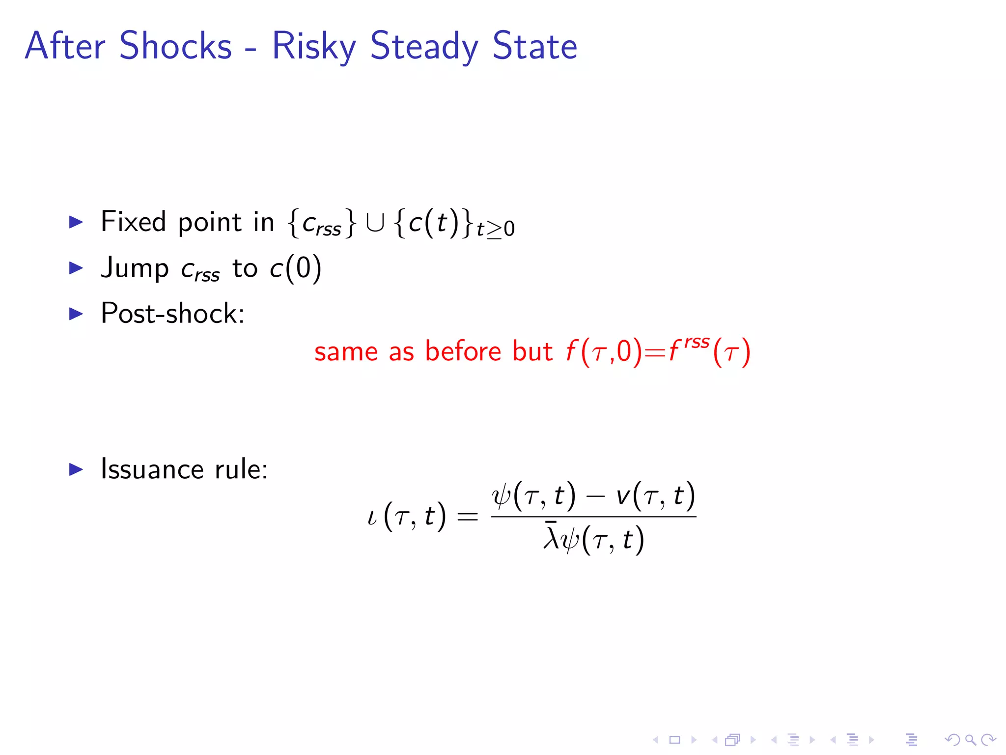
19. Optimal Path
Proposition:
1) v(τ, t) ≡ − j(τ,t)
u (c(t)) solves ‘"ndividual trader” price-PDE:
r(t)
ρ+σ
.
c(t)/c(t)
v (τ, t) = δ +
∂v
∂t
−
∂v
∂τ
, if τ ∈ (0, T]
v (0, t) = 1
2) issuances ι(τ, t):
ι =
ψ (τ, t) − v (τ, t)
¯λψ (τ, t)
3) PDE given f0, c(t) given by BC

20. Asymptotic Properties (t −→ ∞)
1. market and internal valuations:
ψ(τ) = δ
1 − e−¯rss τ
¯rss
+ e−¯rss τ
and v∗
(τ) = δ
1 − e−rss (¯λ)τ
rss(¯λ)
+ e−rss (¯λ)τ
2. issuance:
ι∗
(τ) =
ψ(τ) − v∗(τ)
¯λψ(τ)
.

21. Asymptotic Properties (t −→ ∞)
If ¯λ ≥ ¯λo
rss(λ) = ρ
Steady State c(t) = css > 0
If¯λ < ¯λo
limt→∞C(t) = 0
rss(λ) ∈ [¯rss, ρ)

22. Asymptotic Values - varying ¯λ
Liquidity, 76
0 0.5 1 1.5 2
-0.1
-0.05
0
0.05
0.1
0.15
0.2
0.25
0.3
6o
c1
Liquidity, 76
0 0.5 1 1.5 2
0.04
0.045
0.05
0.055
0.06
6o
r1
Maturity, =
0 5 10 15 20
0
0.05
0.1
0.15
0.2
41
Maturity, =
0 5 10 15 20
0
0.5
1
1.5
2
2.5
f1

23. Steady State (when λ ≥ ¯λo)
Assumption ρ > ¯r
Maturity, =
0 5 10 15 20
0
0.01
0.02
0.03
0.04
0.05
0.06
0.07
Outstanding Debt f(=)
Maturity, =
0 5 10 15 20
#10-3
0
1
2
3
4
5
6
Issuances 4(=)
Maturity, =
0 5 10 15 20
#10-3
0
1
2
3
4
5
6
7
Maturity Distribution
Maturity, =
0 5 10 15 20
0.75
0.8
0.85
0.9
0.95
1
A(=) vs. !v(=)
A(=)
!v(=)

24. Frictionless Benchmark ¯λ = 0
If ψ arbitrage free:
r(t) = ¯r(t),
ψ(τ, t) = v(τ, t)
Discount Factor pins consumption:
.
c(t)
c(t)
= −
ρ − ¯r(t)
σ
Indeterminate maturity!

25. Frictionless Limit ¯λ −→ 0
If ψ arbitrage free
r(t) = ¯r(t),
ψ(τ, t) = v(τ, t)
Discount Factor pins consumption:
.
c(t)
c(t)
= −
ρ − ¯r(t)
σ
Determinate Maturity!

26. Transitional Dynamics - Fixed Point
Input: c(t)
Discount Factor:
r(t) = ρ + σ
.
c(t)
c(t)
Valuations:
r(t)
Value of Debt
v (τ, t) =
Coupon
δ +
dv(τ,t)
dt
∂v
∂t
−
∂v
∂τ
Optimal Issuance:
ι (τ, t) =
ψ(τ, t) − v(τ, t)
¯λψ(τ, t)
Output: c(t) (follows from KFE+BC)

27. Deterministic Dynamics
Application: Transitions

28. Application 1 - Transitions
Transitions reveal two novel features:
1. Income path for y(t)
liquidity cost + finite maturity produce issuance cycle
2. Path for short rate ¯r(t)
show consumption vs. liquidity smoothing

29. Transition after MIT shock to y(t)
Shock %5 output, T = 20
Time, t
0 50 100 150 200
%
5.9
6
6.1
6.2
6.3
6.4
6.5
Time Discount r(t) (bps)
Time, t
0 50 100 150 200
0.85
0.9
0.95
1
c(t) vs. y(t)
c(t) y(t)
Time, t
0 50 100 150 200
%yss
0
0.01
0.02
0.03
0.04
Issuances Rate, 4(t)
Time, t
0 50 100 150 200
%yss
0
0.2
0.4
0.6
0.8
Debt Outstanding, f(t)
0-5 (years) 5-10 10-15 T-5 to T

30. Longer Maturity
Shock %5 output, from T = 20 to T = 30
Time, t
0 50 100 150 200
%
5.9
6
6.1
6.2
6.3
6.4
6.5
Time Discount r(t) (bps)
Time, t
0 50 100 150 200
0.85
0.9
0.95
1
c(t) vs. y(t)
c(t) y(t)
Time, t
0 50 100 150 200
%yss
0
0.01
0.02
0.03
0.04
Issuances Rate, 4(t)
Time, t
0 50 100 150 200
%yss
0
0.2
0.4
0.6
0.8
Debt Outstanding, f(t)
0-5 (years) 5-10 10-15 T-5 to T

31. Transitions after AR(1) MIT shock to ¯r(t)
Rates

32. Transitions after AR(1) MIT shock to ¯r(t)
Optimal Policy
Time, t
0 50 100 150 200
%
4
5
6
7
8
Time Discount r(t) (bps)
Time, t
0 50 100 150 200
0.9
0.95
1
1.05
1.1
1.15
c(t) vs. y(t)
c(t) y(t)
Time, t
0 50 100 150 200
%yss
0
0.02
0.04
0.06
0.08
Issuances Rate, 4(t)
Time, t
0 50 100 150 200
%yss
0
0.2
0.4
0.6
0.8
Debt Outstanding, f(t)
0-5 (years) 5-10 10-15 T-5 to T

33. Transitions after AR(1) MIT shock to ¯r(t)
Infinite IES - when σ=0
Time, t
0 50 100 150 200
%
4
5
6
7
8
Time Discount r(t) (bps)
Time, t
0 50 100 150 200
0.9
0.95
1
1.05
1.1
1.15
c(t) vs. y(t)
c(t) y(t)
Time, t
0 50 100 150 200
%yss
0
0.02
0.04
0.06
0.08
Issuances Rate, 4(t)
Time, t
0 50 100 150 200
%yss
0
0.2
0.4
0.6
0.8
Debt Outstanding, f(t)
0-5 (years) 5-10 10-15 T-5 to T

34. Dynamics under Risk
Theory

35. Risk
What about Risk?
Complication: fixed point in sets of functions
Risky Steady State:
allows analysis with risk

36. Role of Uncertainty - Risky Steady State
Next...
Before shock: yss and ¯rss at steady state
Poisson event with arrival rate θ
After shock:
draw {y (0) ,¯r(0)} ∼ F
{y(t),¯r(t)} → {yss,¯rss}
RSS:
shock expected
t → ∞ before realization
opposite of MIT shock

37. After Shocks - Risky Steady State
Fixed point in {crss} ∪ {c(t)}t≥0
Jump crss to c(0)
Post-shock:
same as before but f (τ,0)=f rss
(τ)
Issuance rule:
ι (τ, t) =
ψ(τ, t) − v(τ, t)
¯λψ(τ, t)

38. Before Shock - Risky Steady State
Risk Adjusted Valuation:
ρvrss (τ) = δ +
∂vrss(τ)
∂τ
+ θ E v (τ, 0)
u (c(0))
u (crss)
− vrss(τ)
HJB solution is:
vrss(τ) =
τ
0
e−(ρ+θ)s
θE v (τ, 0)
u (c(0))
u (crss)
+ δ ds + e−(ρ+θ)τ
Intuition:
One value per shock: v (τ, 0) and c(0)
marginal utility ratio: “exchange-rate” between states

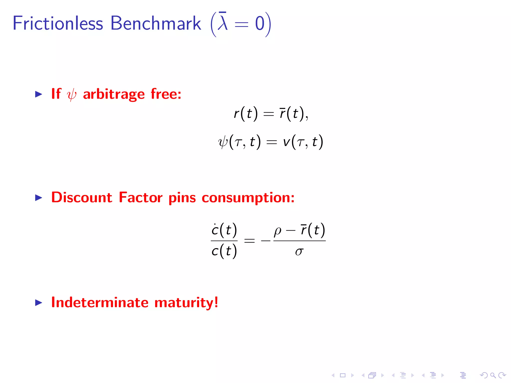
39. Frictionless Limit - Pre-shock Transition
ˆψ (τ, t) = ˆv (τ, t)
Price Equation:
¯r (t) ˆψ (τ, t) = δ +
∂ ˆψ
∂t
−
∂ ˆψ
∂τ
+ θ E [ψ (τ, t)] − ˆψ (τ, t)
HJB and ˆψ (τ, t) = ˆv (τ, t)
r(t) ˆψ (τ, t) = δ +
∂ ˆψ
∂t
−
∂ ˆψ
∂τ
+ θ E
U (c (t))
U (ˆc (t))
ψ (τ, t) − ˆψ (τ, t)
both equations must be consistent

40. Frictionless Limit - Two Polar Cases
Lack of Insurance:
If only y(t) jumps
ψ (τ, t) = ˆψ (τ, t) = 1
r(t) = ¯r(t) + θ E
U (c (t))
U (ˆc (t))
− 1
And an RSS always exists
Complete Insurance:
requires ability to construct portfolio:
such that ˆc (t) = c (t) for all shocks
r(t) = ¯r(t)
Asymptotic Limit, but no RSS

41. Dynamics under Risk
Application 1: SS vs. RSS

42. AR(1) MIT shock to y(t) - RSS vs. SS
Expecting a 5% y(t) drop
Maturity, =
0 5 10 15 20
0
0.01
0.02
0.03
0.04
0.05
0.06
Outstanding Debt f(=)
Maturity, =
0 5 10 15 20
#10-3
0
1
2
3
4
5
Issuances 4(=)
Maturity, =
0 5 10 15 20
#10-3
0
1
2
3
4
5
6
7
Maturity Distribution
Maturity, =
0 5 10 15 20
0.75
0.8
0.85
0.9
0.95
1
A(=) vs. !v(=)
A(=; ss)
A(=; rss)
!v(=; ss)
!v(=; rss)
!v(=; 0)

43. AR(1) MIT shock to y(t) - Transition from RSS
5% Output Shock
Time, t
0 50 100 150 200
%
5.8
5.85
5.9
5.95
6
6.05
6.1
6.15
Time Discount r(t) (bps)
Time, t
0 50 100 150 200
0.94
0.95
0.96
0.97
0.98
0.99
1
c(t) vs. y(t)
c(t)
y(t)
Time, t
0 50 100 150 200
%yss
0
0.005
0.01
0.015
0.02
0.025
Issuances Rate, 4(t)
Time, t
0 50 100 150 200
%yss
0
0.05
0.1
0.15
0.2
0.25
0.3
Debt Outstanding, f(t)
0-5 (years) 5-10 10-15 T-5 to T

44. AR(1) MIT shock to ¯r(t) - RSS vs. SS
Shock 4% to 8% on impact, ρ = 6%
Maturity, =
0 5 10 15 20
-0.01
0
0.01
0.02
0.03
0.04
0.05
0.06
Outstanding Debt f(=)
Maturity, =
0 5 10 15 20
#10-3
-1
0
1
2
3
4
5
Issuances 4(=)
Maturity, =
0 5 10 15 20
-0.015
-0.01
-0.005
0
0.005
0.01
0.015
Maturity Distribution
Maturity, =
0 5 10 15 20
0.7
0.75
0.8
0.85
0.9
0.95
1
A(=) vs. !v(=)
A(=; ss)
A(=; rss)
!v(=; ss)
!v(=; rss)
!v(=; 0)

45. AR(1) MIT shock to ¯r(t) - RSS vs. SS
Shock 4% to 8% on impact, ρ = 6%
Time, t
0 50 100 150 200
%
5.6
5.8
6
6.2
6.4
6.6
6.8
7
Time Discount r(t) (bps)
Time, t
0 50 100 150 200
0.96
0.97
0.98
0.99
1
1.01
c(t) vs. y(t)
c(t)
y(t)
Time, t
0 50 100 150 200
%yss
-0.005
0
0.005
0.01
0.015
0.02
0.025
Issuances Rate, 4(t)
Time, t
0 50 100 150 200
%yss
-0.05
0
0.05
0.1
0.15
0.2
0.25
0.3
Debt Outstanding, f(t)
0-5 (years) 5-10 10-15 T-5 to T

46. Application 1: Lessons
optimal risk management
long-term debt, short-term assets

47. Conclusion
New approach to study maturity
liquidity
continuum of bonds of any class
Can only analyze RSS
Forces at play
liquidity cost vs. consumption smoothing
risk-aversion vs. incentives
Next: default
Future: recent developments to study aggregate shocks

48. Steady State - Comp Stats
Higher differentials ρ − ¯r
amplifies issuances, for higher maturity
Lower λ
scales ι(τ) and f (τ)
Role of T
dilutes adjustment cost

49. Dual
Given {c(t)}t≥0, then planner’s discount:
r(t) = ρ + σ
˙c(t)
c(t)
Dual Problem
D [f (·, 0)] = min
{ι(τ,t)}t=τ∈[0,∞),τ∈[0,T]
∞
0
e−
t
0
r(s)ds
ytdt s.t.
∂f
∂t
= ι (τ, t) +
∂f
∂τ
, f (T, t) = 0; f (τ, 0) = f0(τ)
y (t) = c (t) + f (0, t) −
T
0
[q (τ, t, ι) ι (τ, t) − δf (τ, t)] dτ
back

50. Dual (button)
Given {c(t)}t≥0, then planner’s discount:
r(t) = ρ − σ
˙c(t)
c(t)
Dual:
D [f (·, 0)] = min
{ι(τ,t)}t=τ∈[0,∞),τ∈[0,T]
∞
0
e−
t
0
r(s)ds
(f (0, t)−
T
0
(ψ(τ, t) − λ
∂f
∂t
= ι (τ, t) +
∂f
∂τ
, f (τ, 0) = f0(τ)
back

51. Two Definitions (button)
Yield curve Ψ(τ, t):
Implicit constant rate Ψ(τ, t) that solves:
ψ(τ, t) = e−Ψ(τ,t)τ
+ δ
τ
0
e−Ψ(τ,t)s
ds
Portfolio Weights (maturity distribution):
(τ,t) ≡
f (τ, t)
T
0 f (s, t)ds

52. Two Definitions (button)
Yield curve Ψ(τ, t):
Implicit constant rate Ψ(τ, t) that solves:
ψ(τ, t) = e−Ψ(τ,t)τ
+ δ
τ
0
e−Ψ(τ,t)s
ds
Portfolio Weights (maturity distribution):
(τ,t) ≡
f (τ, t)
T
0 f (s, t)ds

53. Appendix - Debt Evolution
From Discrete time
f (τ, t + dt)
τ−debt tomorrow
= ι(τ, t)dt
new inflow
+ f (τ + dt, t)
becoming τ−debt
Note that dt = −dτ:
f (τ, t + dt) − f (τ, t)
dt
= ι(τ, t) +
f (τ + dt, t) − f (τ, t)
dt
= ι(τ, t) +
f (τ − dτ, t) − f (τ, t)
(−dτ)
Take limit dt → 0
∂f (τ, t)
∂t
= ι (τ, t) +
∂f (τ, t)
∂τ
Back

54. Appendix - Debt Evolution
From Discrete time
f (τ, t + dt)
τ−debt tomorrow
= ι(τ, t)dt
new inflow
+ f (τ + dt, t)
becoming τ−debt
Note that dt = −dτ:
f (τ, t + dt) − f (τ, t)
dt
= ι(τ, t) +
f (τ + dt, t) − f (τ, t)
dt
= ι(τ, t) +
f (τ − dτ, t) − f (τ, t)
(−dτ)
Take limit dt → 0
∂f (τ, t)
∂t
= ι (τ, t) +
∂f (τ, t)
∂τ
Back

55. Appendix - Debt Evolution
From Discrete time
f (τ, t + dt)
τ−debt tomorrow
= ι(τ, t)dt
new inflow
+ f (τ + dt, t)
becoming τ−debt
Note that dt = −dτ:
f (τ, t + dt) − f (τ, t)
dt
= ι(τ, t) +
f (τ + dt, t) − f (τ, t)
dt
= ι(τ, t) +
f (τ − dτ, t) − f (τ, t)
(−dτ)
Take limit dt → 0
∂f (τ, t)
∂t
= ι (τ, t) +
∂f (τ, t)
∂τ
Back

56. Appendix - Debt Evolution
From Discrete time
f (τ, t + dt)
τ−debt tomorrow
= ι(τ, t)dt
new inflow
+ f (τ + dt, t)
becoming τ−debt
Note that dt = −dτ:
f (τ, t + dt) − f (τ, t)
dt
= ι(τ, t) +
f (τ + dt, t) − f (τ, t)
dt
= ι(τ, t) +
f (τ − dτ, t) − f (τ, t)
(−dτ)
Take limit dt → 0
∂f (τ, t)
∂t
= ι (τ, t) +
∂f (τ, t)
∂τ
Back

57. Transitions from an arbitrary f (τ, 0)
Transitional Dynamics from f (τ, 0)=0
Time, t
0 50 100 150 200
%
5.5
5.6
5.7
5.8
5.9
6
Time Discount r(t) (bps)
Time, t
0 50 100 150 200
0.94
0.96
0.98
1
1.02
1.04
1.06
c(t) vs. y(t)
c(t)
y(t)
Time, t
0 50 100 150 200
Issuances
0
0.005
0.01
0.015
0.02
0.025
0.03
Issuances Rate, 4(t)
0-5 year
5-10 years
10-15 years
T-5 to T years
Time, t
0 50 100 150 200
Deviationsfromsteadystate(in%)
0
0.05
0.1
0.15
0.2
0.25
0.3
0.35
Outstanding amounts, f(t)
0-5 year
5-10 years
10-15 years
T-5 to T years
λ smooths adjustment, bullwhip effect, expiration limits debt
accumulation

58. AR(1) MIT shock to y(t) - Risk Neutrality (button)
10% Output Shock
Time, t
0 50 100 150 200
%
6
6.001
6.002
6.003
6.004
6.005
6.006
6.007
Time Discount r(t) (bps)
Time, t
0 50 100 150 200
0.85
0.9
0.95
1
c(t) vs. y(t)
c(t)
y(t)
Time, t
0 50 100 150 200
Outstandingamounts
0.005
0.01
0.015
0.02
0.025
0.03
Issuances Rate, 4(t)
0-5 year
5-10 years
10-15 years
15 6 years
Time, t
0 50 100 150 200
Outstandingamounts
0.05
0.1
0.15
0.2
0.25
0.3
0.35
Issuances Rate, 4(t)
0-5 year
5-10 years
10-15 years
15 6 years

59. AR(1) MIT shock to y(t) - Less Persistence (button)
Same but less persistence
Maturity, =
0 5 10 15 20
0
0.01
0.02
0.03
0.04
0.05
0.06
0.07
Outstanding Debt f(=)
Maturity, =
0 5 10 15 20
#10-3
-1
0
1
2
3
4
5
6
Issuances 4(=)
Maturity, =
0 5 10 15 20
#10-3
0
1
2
3
4
5
6
7
Maturity Distribution
Maturity, =
0 5 10 15 20
0.75
0.8
0.85
0.9
0.95
1
1.05
A(=) vs. !v(=)
A(=; ss)
A(=; rss)
!v(=; ss)
!v(=; rss)

60. Dynamic Hedging - A Combined Shock
A ¯r(t) and y(t) shock combined
Maturity, =
0 5 10 15 20
-0.04
-0.02
0
0.02
0.04
0.06
0.08
Outstanding Debt f(=)
Maturity, =
0 5 10 15 20
#10-3
-2
-1
0
1
2
3
4
5
6
Issuances 4(=)
Maturity, =
0 5 10 15 20
-0.01
-0.005
0
0.005
0.01
Maturity Distribution
Maturity, =
0 5 10 15 20
0.75
0.8
0.85
0.9
0.95
1
A(=) vs. !v(=)
A(=; ss)
A(=; rss)
!v(=; ss)
!v(=; rss)

61. Dynamic Hedging - A Combined Shock
A ¯r(t) and y(t) shock combined
Time, t
0 50 100 150 200
%
5.5
6
6.5
7
7.5
Time Discount r(t) (bps)
Time, t
0 50 100 150 200
0.95
0.96
0.97
0.98
0.99
1
1.01
1.02
c(t) vs. y(t)
c(t)
y(t)
Time, t
0 50 100 150 200
Outstandingamounts
-0.01
-0.005
0
0.005
0.01
0.015
0.02
0.025
0.03
Issuances Rate, 4(t)
0-5 year
5-10 years
10-15 years
15 6 years
Time, t
0 50 100 150 200
Outstandingamounts
-0.2
-0.1
0
0.1
0.2
0.3
0.4
Issuances Rate, 4(t)
0-5 year
5-10 years
10-15 years
15 6 years

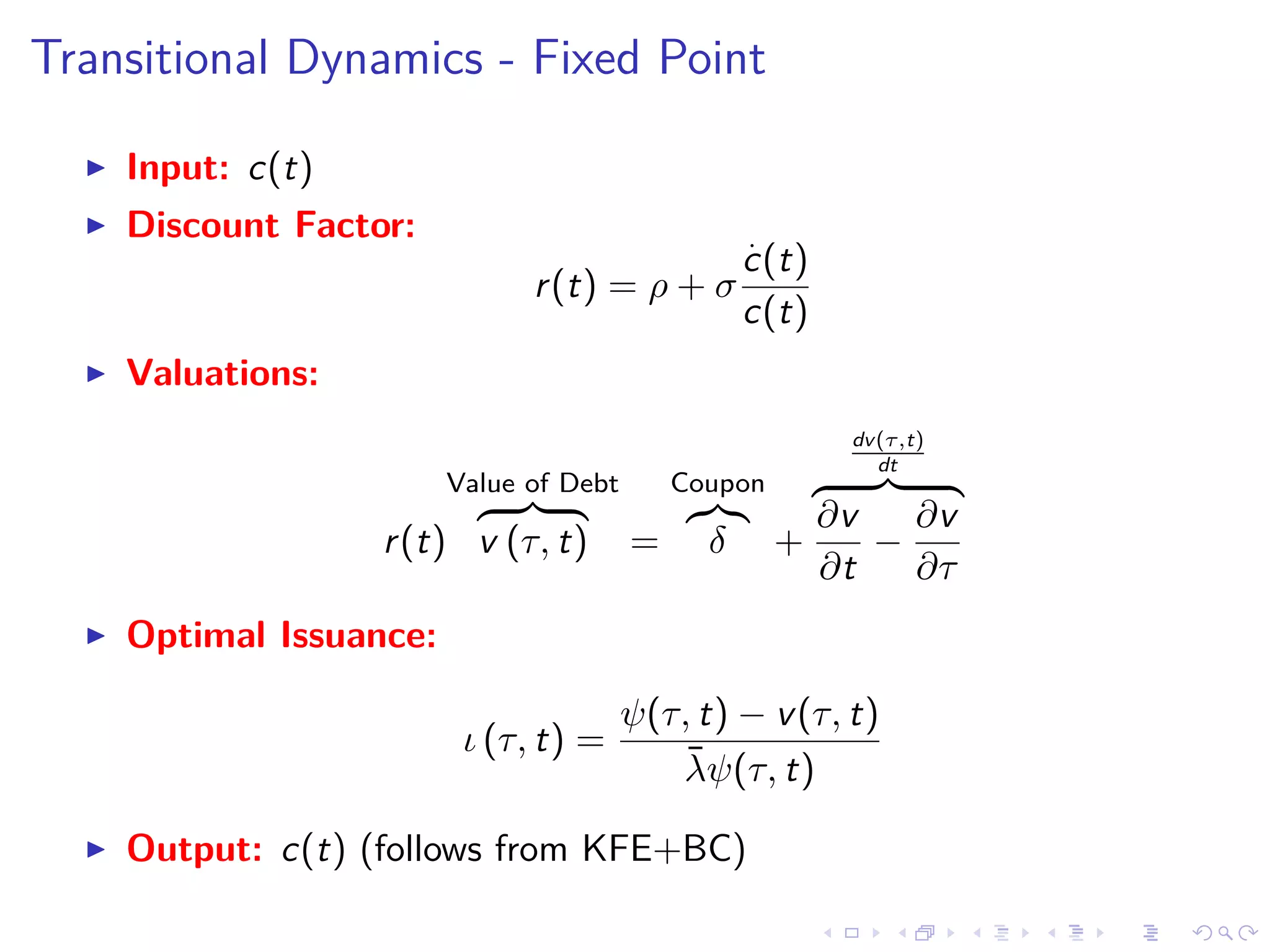
62. Transitional Dynamics - Fixed Point Algorithm in r(t)
1. Build:
r(t) = ρ − σ
˙c(t)
c(t)
2. Plug r(t) into value PDE:
r(t)v (τ, t) = −δ +
∂v
∂t
−
∂v
∂τ
3. Build issuances:
ι (τ, t) =
ψ(τ, t) + v(τ, t)
¯λ
4. Obtain f (t, τ):
f (τ, t) =
min{T,τ+t}
τ
ι(t + τ − s, s)ds + I[T > t + τ] · f (τ + t, 0)
5. c(t) given by
cout
(t) = y (t) − f (0, t) +
T
0
[q (τ, t, ι) ι (τ, t) − δf (τ, t)] dτ

63. Gateaux Derivative of V
dV
df
= lim
α→0
V (f + αh(τ,t)) − V (f )
α
where
h(τ,t)(˜τ,˜t) = Dirac function at (τ, t)
Back