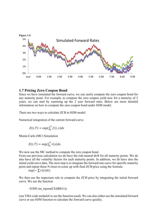
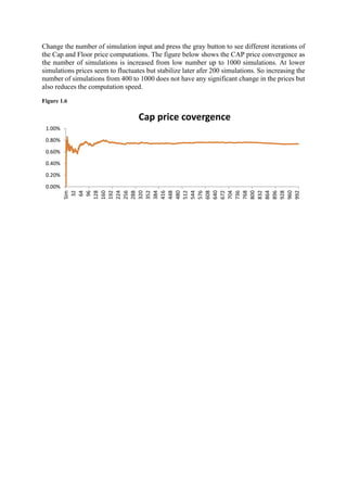
The document discusses implementing the Heath-Jarrow-Morton (HJM) model for modeling interest rate dynamics using Monte Carlo simulation. It describes:
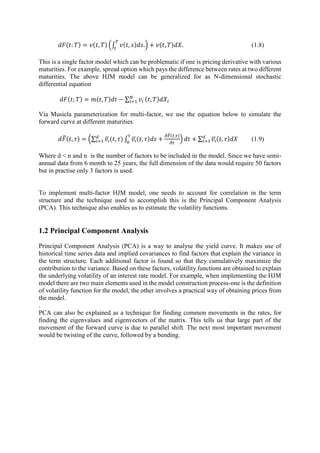
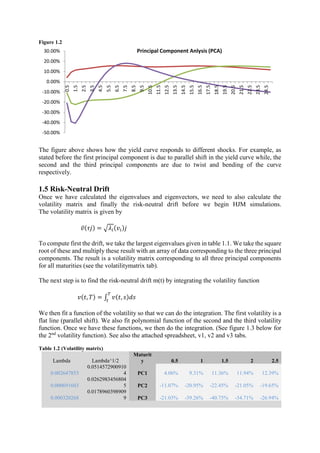
1) Using principal component analysis to analyze the yield curve and estimate volatility functions for a multi-factor HJM model from historical yield curve data.
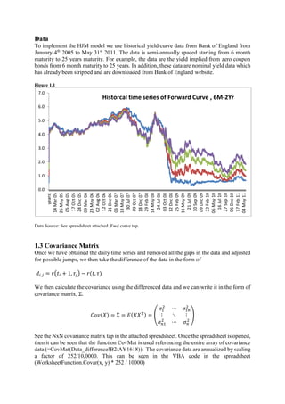
2) Calculating the covariance matrix from differenced historical yield curve data and factorizing it to obtain eigenvalues and eigenvectors via numerical methods.
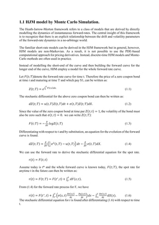
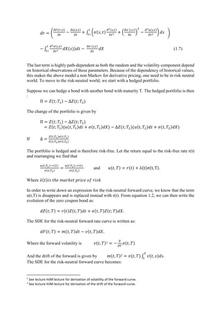
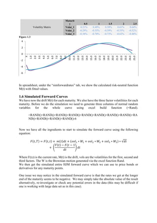
3) Deriving the stochastic differential equation for the risk-neutral forward rate curve under the HJM model using no-arbitrage arguments to obtain drift and volatility terms.