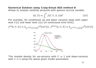
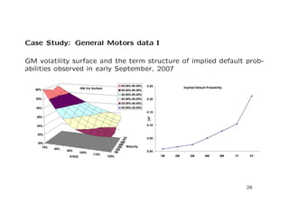
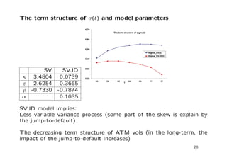
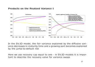
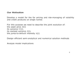
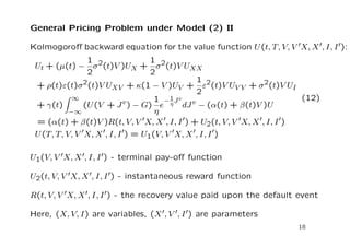
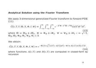
The document discusses a stochastic volatility model that incorporates jumps in volatility and the possibility of default. It describes the dynamics of the model and how it can be used to price volatility and credit derivatives. Analytical and numerical methods are presented for solving the pricing problem. As an example application, the model is fit to data on General Motors to analyze the implications.

1. Volatility derivatives and default risk
ARTUR SEPP
Merrill Lynch
Quant Congress London
November 14-15, 2007
1

2. Plan of the presentation
1) Heston stochastic volatility model with the term-structure of ATM
volatility and the jump-to-default: interaction between the realized
variance and the default risk
2) Analytical and numerical solution methods for the pricing problem
3) Case study: application of the model to the General Motors data,
implications
2

3. References
Theoretical and practical details for my presentation can be found in:
1) Sepp, A. (2008) Pricing Options on Realized Variance in the He-
ston Model with Jumps in Returns and Volatility, Journal of Compu-
tational Finance, Vol. 11, No. 4, pp. 33-70
http://ssrn.com/abstract=1408005
2) Sepp, A. (2007) Ane Models in Mathematical Finance: an An-
alytical Approach, PhD thesis, University of Tartu
http://math.ut.ee/~spartak/papers/seppthesis.pdf
3) Sepp, A. (2006) Extended CreditGrades Model with Stochastic
Volatility and Jumps, Wilmott Magazine, September, 50-60
http://ssrn.com/abstract=1412327
3

4. Financial Motivation
Volatility Products
Hedging against changes in the realized/implied volatility
Speculation and directional trading
Credit Default Swaps
Hedging against the default of the issuer
Speculation and directional trading
Volatility and Credit Products
The degree of correlation ?
Relative value analysis
4

5. Volatility Products I
The asset realized variance:
IN(t0; tN) =
AF
N
NX
n=1
ln
S(tn)
S(tn1)
!2
; (1)
S(tn) is the asset closing price observed at times t0 (inception); ::; tN
(maturity)
N is the number of observations
AF is annualization factor (typically, AF=252 - daily sampling)
Realized variance swap with payo function:
U(T; I) = IN(0; T) K2
fair
K2
fair - the fair variance which equates the value of the var swap at
the inception to zero
Call on the realized variance swap with payo function:
U(T; I) = max
IN(0; T) K2
fair; 0
5

6. Volatility Products II
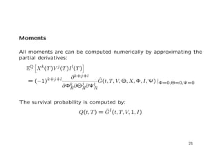
Forward-start call:
U(TF ; T) = max
S(T)
S(TF )
K; 0
!
where TF - forward start time, T - maturity
Forward-start variance swap:
U(TF ; T) = IN(TF ; T) K2
fair
Option on the future implied volatility (VIX-type option):
U(T; T) = max
q
E[IN(T; T +T)] K; 0
The values of these products are sensitive to the evolution of the
volatility surface
6

7. Credit Products
Credit default swap (CDS) - the protection against the default of
the reference name in exchange for quarterly coupon payments
Deep out-of-the money put option - tiny value under the log-
normal model unless a huge volatility parameter is used
The value of a deep OTM put is almost proportional to its strike and
the default probability up to its maturity
Forward-start options - would typically lose their value if the default
occurs up to the forward-start date
The value of the forward-start option is sensitive to the evolution of
the default probability curve
7

8. Our Motivation
Develop a model for the for pricing and risk-managing of volatility
and credit products on single names
For this purpose we need to describe the joint evolution of:
the asset price S(t)
its variance V (t),
its realized variance I(t),
the jump-to-default intensity (t)
Design ecient semi-analytical and numerical solution methods
Analyze model implications
8

9. Heston model with volatility jumps and jump-to-default I
We adopt the following joint dynamics under the pricing measure Q:
dS(t)
S(t)
q
V (t)dWs(t) dNd(t); S(0) = S0
= (t)dt+(t)
q
V (t)dWv(t)+JvdNv(t); V (0) = 1;
dV (t) = (1 V (t))dt+(t)
dI(t) = 2(t)V (t)dt; I(0) = I0;
(t) = (t)+

10. (t)V (t);
(2)
V (t) is normalized variance
(t) - is ATM-volatility
Nd(t) - Poisson process with intensity (t)
minf : Nd() = 1g is the default time
9

11. Heston model with volatility jumps and jump-to-default II
(t) = r(t) d(t)+(t) - the risk-neutral drift
(t) - the instantaneous correlation between Ws(t) and Wv(t)
Nv(t) - Poisson process with intensity
Jv - the exponential jump with mean
(t) - the vol-vol parameter
- the mean-reversion
10

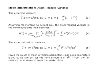
12. Model Interpretation: Asset Realized Variance
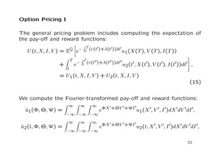
The expected variance:
V (T) := EQ[V (T)jV (0) = 1] = 1+
1 eT
(3)
Assuming for moment no default risk, the asset realized variance in
the continuous-time limit becomes:
I(T) = lim
N!1
X
tn2N
ln
S(tn)
S(tn1)
!2
=
Z T
0
2(t0)V (t0)dt0 (4)
The expected realized variance:
I(T) := EQ[I(T)jV (0) = 1] =
Z T
0
2(t0)V (t0)dt0 (5)
Given the values of mean-reversion parameters and jump parameters
and
, we can extract the term structure of 2(t) from the fair
variance curve observed from the market data
11

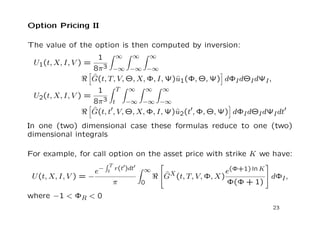
13. Model Interpretation: Jump-to-Default
The probability of survival up to time T:
Q(t; T) = EQ[ Tj t] = EQ[e
R T
t (t0)dt0
] (6)
The probability of defaulting up to time T is connected to the inte-
grated expected variance:
Qc(t; T) = EQ[ Tj t] = 1Q(t; T)
Z T
t
((t0)+

14. (t0)V (t0))dt0 (7)
Variation of the default intensity:
(t) =

15. 2 V (t) (8)
Parameter

16. can be extracted form the time series or from non-linear
CDS contracts
The term structure of parameter (t), is backed-out from the survival
probabilities implied CDS quotes
12

17. Recovery Assumption I
Should be speci

18. ed by the contract terms
Can be simpli

19. ed by the modeling purposes
Asset price: zero
Call option payo: zero
Put option payo: its strike
Forward-start call option payo: zero
Forward-start put option: zero if defaulted before the forward-
start date, its strike if defaulted between the forward-start date and
maturity
13

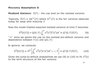
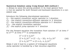
20. Recovery Assumption II
Realized Variance: ^I(T) - the cap level on the realized variance
Typically, ^I(T) = 3KV (T) where KV (T) is the fair variance observed
today for swap with maturity T
Now the model implied expected realized variance at time T becomes:
EQ[I(T)] Q(0; T)
Z T
0
2(t0)V (t0)dt0 +Qc(0; T)^I(T); (9)
since we ignore the cap on the realized pre-default variance and
dependence between V (t) and Q(t; T)
In general, we compute:
EQ[I(T)] = EQ
Z T
0
2(t0)V (t0)dt0 j T
#
+Qc(0; T)^I(T); (10)
Given the jump-to-default probabilities we use (9) or (10) to

21. t 2(t)
to the term structure of the fair variance
14

22. Model Interpretation: Volatility Jumps
Introduce the fat right tail to the density of the variance
Explain the positive skew observed in the VIX options
At the same time:
Decrease the (terminal) correlation between the spot and both the
implied variance and realized variance
Increase the variance of the realized variance while give little impact
on the asset (terminal) variance
As a result, calibrating the variance jumps to the deep skews is not
reasonable - we need to calibrate them to the volatility products
15

23. Convergence of Discretely Sampled Realized Variance to Con-
tinuous Time Limit, T = 1y, S0 = 1, V0 = 1, = 0:05, = 0:2,
= 2, = 1, = 0:8,
= 0:5, = 1
As the number of

24. xings decreases, the mean of the discrete sample
decreases while its variance increases
16

25. General Pricing Problem under Model (2) I
For calibration and pricing we need to model the joint evolution of
(X(t); V (t); I(t)) with X(t) = ln S(t)
Kolmogoro forward equation for the joint transition density function
G(t; T; V; V 0;X;X0; I; I0):
GT
((T)
1
2
2(T)V 0)G
X0
+
1
2
2(T)V 0G
X0X0
+
(T)(T)2(T)V 0G
X0V 0 +
(1 V 0)G
V 0 +
1
2
2(T)V 0G
V 0V 0
(T)V 0G
I0
(T)
Z 1
0
(G(V Jv) G)
1
1
e
Jv
dJv
((T)+

26. (T)V 0)G = 0;
G(t; t; V; V 0X;X0; I; I0) = (X0 X)(V 0 V )(I0 I);
(11)
Here, (X0; V 0; I0) are variables (future states of the world), (X; V; I)
are initial data
17

27. General Pricing Problem under Model (2) II
Kolmogoro backward equation for the value function U(t; T; V; V 0X;X0; I; I0):
Ut +((t)
1
2
2(t)V )UX +
1
2
2(t)V UXX
+(t)(t)2(t)V UXV +(1 V )UV +
1
2
2(t)V UV V +2(t)V UI
+
(t)
Z 1
1
(U(V +Jv) G)
1
1
e
Jv
dJv ((t)+

28. (t)V )U
= ((t)+

29. (t)V )R(t; V; V 0X;X0; I; I0)+U2(t; V; V 0X;X0; I; I0)
U(T; T; V; V 0X;X0; I; I0) = U1(V; V 0X;X0; I; I0)
(12)
U1(V; V 0X;X0; I; I0) - terminal pay-o function
U2(t; V; V 0X;X0; I; I0) - instantaneous reward function
R(t; V; V 0X;X0; I; I0) - the recovery value paid upon the default event
Here, (X; V; I) are variables, (X0; V 0; I0) are parameters
18

30. Analytical Solution using the Fourier Transform
We apply 3-dimensional generalized Fourier transform to forward PDE
(11):
bG
(t; T; V;;X;; I; ) =
Z 1
1
Z 1
1
Z 1
1
eX0V 0I0 GdX0dV 0dI0;
(13)
where = R + iI; = R + iI; = R + i I i =
p
1,
R;I;R;I; R; I 2 R
We obtain:
bG
(t; T; V;;X;; I; ) = e(X+
R T
t (r(t0)d(t0))dt0) I+A(t;T)+B(t;T )V ;
(14)
where functions A(t; T) and B(t; T) are computed in closed-form by
recursion
19

31. Marginal Transition Densities and Convergence
Asymptotic convergence rate is important to set-up the bounds for
quadrature and FFT inversion methods
We

32. rst recall that for the Black-Scholes model with constant V :
bG
X(t; T; V;;X) e1
22V02I
; jIj ! 1
For our model we obtain:
bG
X(t; T; V;;X) = bG(t; T; V; 0;X;; I; 0) e
((Tt)+2V0)(12)
jIj; jIj ! 1
bG
I(t; T; V; ; I) = bG
(t; T; V; 0;X; 0; I; ) e
2(Tt)+2V0
2
p
j Ij
; j Ij ! 1;
bG
2
2 ln jIj
V (t; T; V;) = bG
(t; T; V;;X; 0; I; 0) e
; jIj ! 1
x =
R T
0 x(t0)dt0 and stands for the leading term of the real part
In relative terms, the convergence is fast for bG
X, moderate for bG
I,
and slow for bG
V
20

33. Moments
All moments are can be computed numerically by approximating the
partial derivatives:
h
i
EQ
Xk(T)V j(T)Il(T)
= (1)k+j+l @k+j+l
@k
R@j
R@ l
R
bG
(t; T; V;;X;; I; ) j=0;=0; =0
The survival probability is computed by:
Q(t; T) = bG
I(t; T; V; 1; I)
21

34. Option Pricing I
The general pricing problem includes computing the expectation of
the pay-o and reward functions:
U(t;X; I; V ) = EQ
e
R T
t (r(t0)+(t0))dt0
u1(X(T); V (T); I(T))
+
Z T
t
e
R t0
t (r(t00)+(t00))dt00
u2(t0;X(t0); V (t0); I(t0))dt0
#
;
= U1(t;X; I; V )+U2(t;X; I; V )
(15)
We compute the Fourier-transformed pay-o and reward functions:
bu
1(;; ) =
Z 1
1
Z 1
1
Z 1
1
eX0+V 0+ I0
u1(X0; V 0; I0)dX0dV 0dI0;
bu
2(t;;; ) =
Z 1
1
Z 1
1
Z 1
1
eX0+V 0+ I0
u2(t;X0; V 0; I0)dX0dV 0dI0;
22

35. Option Pricing II
The value of the option is then computed by inversion:
U1(t;X; I; V ) =
1
83
Z 1
1
Z 1
1
Z 1
1
h
bG
(t; T; V;;X;; I; )bu
1(;; )
i
dIdId I;
U2(t;X; I; V ) =
1
83
Z T
t
Z 1
1
Z 1
1
Z 1
1
h
bG
(t; t0; V;;X;; I; )bu
2(t0;;; )
i
dIdId Idt0
In one (two) dimensional case these formulas reduce to one (two)
dimensional integrals
For example, for call option on the asset price with strike K we have:
U(t;X; I; V ) =
e
R T
t r(t0)dt0
Z 1
0
2
4bG
X(t; T; V;;X)
e(+1) lnK
(+1)
3
5 dI;
where 1 R 0
23

36. Numerical Solution using Craig-Sneyd ADI method I
Allows to solve the pricing problem in its most general form
Can be applied for both forward and backward equations in a con-
sistent way
Introduce the following discretesized operators:
LI - the explicit convection vector operator in I direction
LX - the implicit convection-diusion operator in X direction
LV - the implicit convection-diusion operator in V direction
CXV - the explicit correlation operator
JV - the explicit jump operator in V direction
For the forward equation the transition from solution Gn at time tn
to Gn+1 at time tn+1 is computed by:
G = (I +LI)Gn
(I +LX)G = (I LX 2LV +CXV )G
(I +LV )Gn+1 = (I +LV +JV )G
(16)
Steps 2 and 3 lead to a system of tridiagonal equations
Jump operator is handled by a fast recursive algorithm
24

37. Numerical Solution using Craig-Sneyd ADI method II
Allows to analyze volatility products with general accrual variable:
I(t; T) =
Z T
t
f(t0; V;X; I)dt0 (17)
For example, for conditional up and down variance swap with upper
level U(t) and lower level L(t) (in continuous time limit):
fup(t; V;X) = 1feX(t)U(t)g2(t)V (t); fdown(t; V;X) = 1feX(t)L(t)g2(t)V (t)
The implied density for up-variance with U = 1 and down-variance
with L = 1 using the above given model parameters
25

38. Case Study: General Motors data I
GM volatility surface and the term structure of implied default prob-
abilities observed in early September, 2007
26

39. Case Study: General Motors data II
For illustration we calibrate two models:
1) SV - the dynamics (2) without jump-to-default
2) SVJD - the dynamics (2) with jump-to-default
The term structure of (t) is backed-out from the ATM volatilities,
other parameters are kept constant, no volatility jumps
Jump-to-default intensity parameter is inferred from the term struc-
ture of implied probabilities for GM CDS (which is pretty
at),

40. = 0
27

41. The term structure of (t) and model parameters
SV SVJD
3.4804 0.0739
2.6254 0.3665
-0.7330 -0.7874
0.1035
SVJD model implies:
Less variable variance process (some part of the skew is explain by
the jump-to-default)
The decreasing term structure of ATM vols (in the long-term, the
impact of the jump-to-default increases)
28