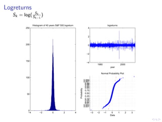
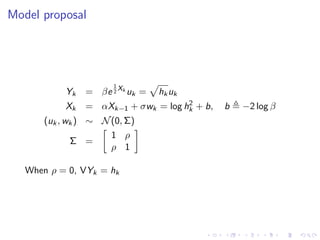
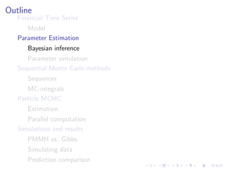
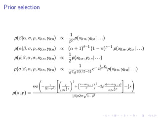
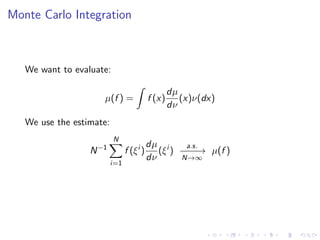
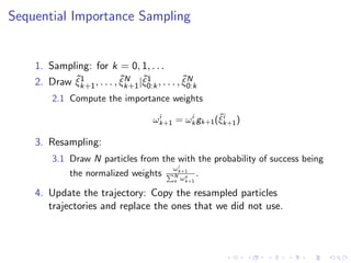
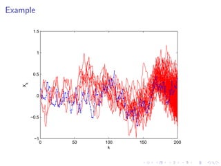
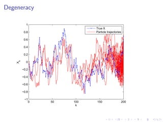
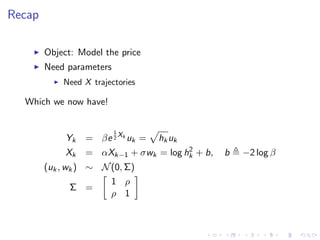
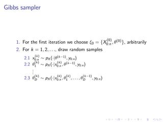
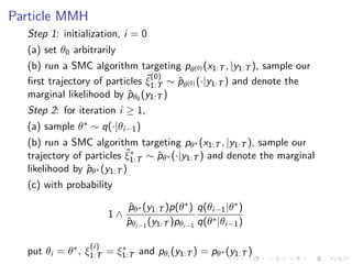
Bayesian Inference on a Stochastic Volatility model Using PMCMC methods

Bayesian Inference on a Stochastic Volatility
model Using PMCMC methods

Jonas Hallgren

August 1, 2011

Outline
Financial Time Series
Model
Parameter Estimation
Bayesian inference
Parameter simulation
Sequential Monte Carlo methods
Sequences
MC-integrals
Particle MCMC
Estimation
Parallel computation
Simulations and results
PMMH vs. Gibbs
Simulating data
Prediction comparison

Financial Time series
9 S&P500 Daily returns
x 10
12

10

8

6

4

2

0
2004 2006 2008 2010

Modeling

We want to model the price of an instrument in order to be able
to:
Price options
Evaluate future risks
Predict future prices

Logreturns
Sk = log( SSk )
k−1

Histogram of 40 years S&P 500 logreturn logreturns
250 4

2

200 0

−2

150
−4
1980 2000
year

Normal Probability Plot
100
0.999
0.997
0.99
0.98
0.95
0.90
Probability

0.75
50 0.50
0.25
0.10
0.05
0.02
0.01
0.003
0.001
0
−4 −2 0 2 4 −3 −2 −1 0 1 2 3
Data

Model proposal

1
Yk = βe 2 Xk uk = hk uk
2
Xk = αXk−1 + σwk = log hk + b, b −2 log β
(uk , wk ) ∼ N (0, Σ)
1 ρ
Σ =
ρ 1

When ρ = 0, VYk = hk

Prior selection

1
p(β|α, σ, ρ, x0:n , y0:n ) ∝ p(x0:n , y0:n | . . .)
β2
p(α|β, σ, ρ, x0:n , y0:n ) ∝ (α + 1)δ−1 (1 − α)γ−1 p(x0:n , y0:n | . . .)
1
p(ρ|β, α, σ, x0:n , y0:n ) ∝ p(x0:n , y0:n | . . .)
2
1 1
p(σ|β, α, ρ, x0:n , y0:n ) ∝ 2 σ 2(t/2−1)
e − 2σ2 S0 p(x0:n , y0:n | . . .)
σ
   
2
x−αxk−1 2 y (x−αxk−1 )
1 y − 1 x 
exp−  + −2ρ
2(1−ρ2 ) 1x σ 1x 2
βe 2 σβe 2
p(x, y ) = √
|β|σ2π 1−ρ2

Gibbs sampler

(0)
1. For the ﬁrst iteration we choose ξ0 = {X0:n , θ(0) }, arbitrarily
2. For k = 1, 2, . . ., draw random samples
(k)
2.1 x0:n ∼ pX (·|θ(k−1) , y0:n )
(k) (k)
2.2 θ1 ∼ pX (·|x0:n , θ(k−1) , y0:n )
.
.
.
(k) (k) (k) (k−1)
2.3 θD ∼ pX (·|x0:n , θ1 , . . . , θD , y0:n )

New problem: How do we sample θ and x?

Metropolis-Hastings sampler

Choose θ0 arbitrarily then for k = 0, ..., N
1. Simulate θ∗ ∼ q(·, θk−1 )
2. with probability
p(θ∗ )q(θ∗ , θk )
1∧
p(θk )q(θk , θ∗ )
set θk+1 = θ∗ , otherwise set θk+1 = θk .

SMC

φk p(xk |y0:k )

Propose:
´
˜
lk−1 (ξ, ξ)φk−1 (ξ)dξ
˜
φk (ξ) = ´ ´
˜ ˜
φk−1 (ξ) lk−1 (ξ, ξ)d ξdξ

Monte Carlo Integration

We want to evaluate:
ˆ
dµ
µ(f ) = f (x) (x)ν(dx)
dν
We use the estimate:
N
dµ i a.s.
N −1 f (ξ i ) (ξ ) − − → µ(f )
−−
dν N→∞
i=1

Sequential Importance Sampling

1. Sampling: for k = 0, 1, . . .
˜1 ˜N ˜1 ˜N
2. Draw ξk+1 , . . . , ξk+1 |ξ0:k , . . . , ξ0:k
2.1 Compute the importance weights
i i ˜i
ωk+1 = ωk gk+1 (ξk+1 )

3. Resampling:
3.1 Draw N particles from the with the probability of success being
i
ωk+1
the normalized weights N s .
s ωk+1

4. Update the trajectory: Copy the resampled particles
trajectories and replace the ones that we did not use.

Example

1.5

1

0.5
k
X

0

−0.5

−1
0 50 100 150 200
k

Degeneracy

1
True X
0.8 Particle trajectories

0.6

0.4

0.2
Xk

0

−0.2

−0.4

−0.6

−0.8

−1
0 50 100 150 200
k

Recap

Object: Model the price
Need parameters
Need X trajectories

Which we now have!

1
Yk = βe 2 Xk uk = hk uk
2
Xk = αXk−1 + σwk = log hk + b, b −2 log β
(uk , wk ) ∼ N (0, Σ)
1 ρ
Σ =
ρ 1

Gibbs sampler

(0)
1. For the ﬁrst iteration we choose ξ0 = {X0:n , θ(0) }, arbitrarily
2. For k = 1, 2, . . ., draw random samples
(k)
2.1 x0:n ∼ pX (·|θ(k−1) , y0:n )
(k) (k)
2.2 θ1 ∼ pX (·|x0:n , θ(k−1) , y0:n )
.
.
.
(k) (k) (k) (k−1)
2.3 θD ∼ pX (·|x0:n , θ1 , . . . , θD , y0:n )

Particle MMH
Step 1: initialization, i = 0
(a) set θ0 arbitrarily
(b) run a SMC algorithm targeting pθ(0) (x1:T , |y1:T ), sample our
˜(0)
ﬁrst trajectory of particles ξ1:T ∼ pθ(0) (·|y1:T ) and denote the
ˆ
marginal likelihood by pθ0 (y1:T )
ˆ
Step 2: for iteration i ≥ 1,
(a) sample θ∗ ∼ q(·|θi−1 )
(b) run a SMC algorithm targeting pθ∗ (x1:T , |y1:T ), sample our
˜∗
trajectory of particles ξ1:T ∼ pθ∗ (·|y1:T ) and denote the marginal
ˆ
likelihood by pθ∗ (y1:T )
ˆ
(c) with probability

pθ∗ (y1:T )p(θ∗ ) q(θi−1 |θ∗ )
ˆ
1∧
pθi−1 (y1:T )pθi−1 q(θ∗ |θi−1 )
ˆ

(i)
put θi = θ∗ , ξ1:T = ξ1:T and pθi (y1:T ) = pθ∗ (y1:T )
∗

UPPMMH

1:C
1. For t = 0, Choose τ1:N arbitrarily (preferably through an
PMMH-sampler)
2. For t = 1, 2, ..., M
2.1 Simulation step, takes time but does not decrease eﬃciency as
C increases: For γ = 1, 2, . . . , C
γ γ γ
2.1.1 Sample τNt ∼ r1:N·t (y , τt·N )
2.2 Merging step, assumed to take zero time to compute: Sample
a multidimensional, multinomial variable A1:C taking values in
t
1, . . . , C with equal probability.
2.3 for γ = 1, 2 . . . , C
γ
γ A
t
2.3.1 put τ1:N·t = τ1:N·t

3. Sample a multinomial variable Aout taking values in 1, . . . , C
t
out
out = τ At
with equal probability and put τ1:K 1:K

PRPMMH
1:C
1. For t = 0, Choose τ1:N arbitrarily (preferably through an
PMMH-sampler)
2. For t = 1, 2, ..., M
2.1 For γ = 1, 2, . . . , C
γ γ γ
2.1.1 Sample (ω γ , τNt ) ∼ r1:N·t (y , τt·N )
2.2 Normalize weights and resample
ω (γ)
2.2.1 For γ = 1, 2, . . . , C put ω (γ) =
¯ (j)
j ω
2.2.2 Sample a multidimensional, multinomial variable A1:C taking t
values in 1, . . . , C with probability (¯ (1) , ω (2) , . . . , ω (M) )
ω ¯ ¯
2.3 for γ = 1, 2 . . . , C
γ γ
γ A A
2.3.1 put τ1:N·t = (τ1:N·t , τNtt )
t

3. Sample a multinomial variable Aout taking values in 1, . . . , C
t
out Aout
t
with equal probability and put τ1:K = τ1:K

Implementation
X0 = randn(C,T); theta0 = randn(C,n_theta);
X(:,1) = X0; theta(:,1) = theta0;
for t = 2:M
% Simulationstep
parfor gamma = 2:C % Parallell for-loop
[X(gamma,Nt) theta(gamma,Nt) omega(gamma)] ...
= PMMH_SAMPLER(X(gamma,t), theta(gamma,t), N);
end
% Mergestep
A = randsample(1:C, C, true, omega/sum(omega))
X(:,1:N*t) = X(A,1:N*t);
theta(:,1:t) = theta(A,1:t);
end
A_out = randsample(1:C,1)
tau_out = [X(A_out,:); theta(A_out,:)];

Gibbs

4000 6000

3000
4000
2000
2000
1000

0 0
0 0.5 1 0.4 0.6 0.8 1
α β

3000 6000

2000 4000

1000 2000

0 0
−1 −0.5 0 0.5 1 0 0.1 0.2 0.3 0.4
ρ σ

PMMH

4000 10000

8000
3000
6000
2000
4000
1000
2000

0 0
0 0.5 1 0 0.5 1
α β

3000 6000

2000 4000

1000 2000

0 0
−1 −0.5 0 0.5 1 0 0.2 0.4 0.6 0.8
ρ σ

S&P500

1
Simulated
0.8 Real

0.6

0.4

0.2

0

−0.2

−0.4

−0.6

−0.8

−1
0 10 20 30 40 50 60 70 80 90 100

Risk measure comparison

VaR and ES answers two questions:
1. VaR: At least how large will a tail event that occurs with
some speciﬁc probability occur?
2. Given such a tail event, how large do we expect the loss to
be? Expressed in mathematical terms: ES EY · IY <VaR
Model VaR ES
Empirical −0.2581 −0.3766
SVOL −0.2781 − 0.2772 −0.3561 − 0.3550
SVOLρ=0 −0.2735 − 0.2728 −0.3484 − 0.3474

Prediction results
RMSE MAE
Dataset Model Qr PPV
(10−3 ) (10−3 )
GBP/USD SVOL 11.706 8.417 0.1753 0.55
GBP/USD SVOLρ=0 11.714 8.420 ∼ ∼
GBP/USD Long 11.714 8.421 −0.2821 ∼
BIDU SVOL 20.188 15.503 0.1302 0.53
BIDU SVOLρ=0 20.232 15.535 ∼ ∼
BIDU Long 20.231 15.531 −0.3031 ∼
S&P500 SVOL 252.94 175.72 0.0825 0.52
S&P500 SVOLρ=0 252.93 175.78 ∼ ∼
S&P500 Long 252.93 175.80 −0.4821 ∼
S&P500 Longµ 252.91 175.72 ∼ ∼
XBC /USD SVOL 5.5762 3.1417 0.2621 0.35
XBC /USD SVOLρ=0 5.5908 3.1347 ∼ ∼
XBC /USD Long 5.5920 3.1323 −0.0477 ∼

Conclusions

PMMH is nice.
Correlation is relevant in price behavior.
Predict risk, perhaps not price.

Bayesian Inference on a Stochastic Volatility model Using PMCMC methods

More Related Content

What's hot

Similar to Bayesian Inference on a Stochastic Volatility model Using PMCMC methods

Recently uploaded

Bayesian Inference on a Stochastic Volatility model Using PMCMC methods