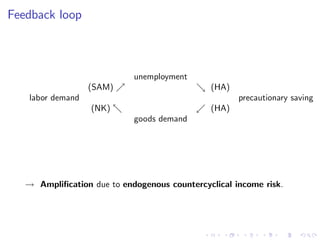
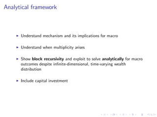
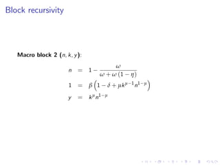
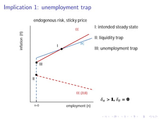
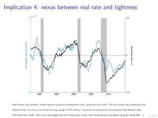
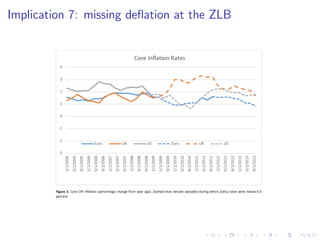
This document summarizes an analytical framework for studying macroeconomic fluctuations combining heterogeneous agent models (HANK) with search and matching frictions in the labor market (SAM). It shows that the interaction between endogenous income risk from SAM unemployment and precautionary savings from HANK can amplify business cycles. Specifically, it finds that this interaction can lead to an unemployment trap, cause a breakdown of the Taylor principle, amplify shock responses, and create a positive nexus between labor market tightness and the real interest rate due to time-varying unemployment risk. The framework is calibrated to match U.S. macro data and its implications are derived both analytically and quantitatively.

1. Macroeconomic Fluctuations with HANK &
SAM: an Analytical Approach
Morten O. Ravn (UCL,CEPR,ADEMU) and Vincent Sterk
(UCL,CEPR,ADEMU)
ADEMU/EUI confernce on Winners, Losers and Policy Reforms after
the Euro crisis
November 2017

2. Contribution
O¤er analytical framework to study macroeconomic ‡uctuations and
policy.
Ingredients:
I Heterogeneous Agents (HA)
I New Keynesian nominal rigidities (NK)
I Search And Matching (SAM).
Show that interaction between HANK & SAM has important
implications for macro.

3. Feedback loop
unemployment
(SAM) % & (HA)
labor demand precautionary saving
(NK) - . (HA)
goods demand
! Ampli…cation due to endogenous countercyclical income risk.

4. Analytical framework
I Understand mechanism and its implications for macro
I Understand when multiplicity arises
I Show block recursivity and exploit to solve analytically for macro
outcomes despite in…nite-dimensional, time-varying wealth
distribution
I Include capital investment

5. Large implications for macro outcomes
1. Emergence Unemployment Trap
2. Breakdown Taylor Principle
3. Ampli…cation Mechanism (Employment & Investment)
4. Tightness - Real Interest Rate Nexus
5. In‡ationary Impact Productivity Shocks
6. Sources of ZLB
7. Missing De‡ation at the ZLB
8. Overturn Supply Shock Paradox
9. Endogenous Risk Premia
! All derive from endogenous countercyclical risk due to
HANK+SAM

6. Literature
I HANK: Gali, Lopez-Salido and Valles (2004), Bilbiie (2008), Auclert
(2015), Bayer, Pham-Dao, Luetticke and Tjaden (2015), Beaudry,
Galizia and Portier (2014), Challe, Matheron, Ragot and
Rubio-Ramirez (2016), Heathcote and Perri (2015), Werning (2015),
Gornemann, Kuester and Nakajima (2016), Guerrieri and Lorenzoni
(2016), Kaplan, Moll and Violante (2016), Luetticke (2015), McKay,
Nakamura and Steinsson (2016), McKay and Reis (2016), Bilbiie
and Ragot (2016), Farhi and Werning (2017), Auclert and Rognlie
(2017), Hagedorn, Manovskii and Mitman (2017), Hedlund,
Mitman, Karahan and Ozkan (2017), Legrand and Ragot (2017),
Farhi and Werning (2017), etc. etc.
I HANK & SAM: Ravn and Sterk (2012), Challe, Matheron, Ragot
and Rubio-Ramirez (2014), Berger, Dew-Becker, Schmidt and
Takahasi (2016), Den Haan, Rendahl and Riegler (2015), Kekre
(2015), McKay and Reis (2016), Auclert and Rognlie (2017), Challe
(2017), etc. etc.

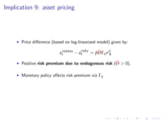
7. Preferences
I continuum of single-member households, indexed by i 2 [0, 1]
I utility:
Vi,t = Et
∞
∑
s=t
βs t
c1 σ
i,s 1
1 σ
ζni,s
!
,
I consumption:
ci,s =
Z
j
cj
i,s
1 1/γ
dj
1/(1 1/γ)
I employment status:
ni,s =
0 if not employed at date s
1 if employed at date s
I receive wi,s when employed, produce ϑ at home if not employed

8. Production technology
I production technology of …rm j:
yj,s = exp (As ) k
µ
j,s n
1 µ
j,s
nj,s = (1 ω)nj,s 1 + hj,s
kj,s = (1 δ)kj,s 1 + ij,s
I Firm owns stock of physical capital (kj ) employee capital (nj )
I TFP (As ) follows AR(1)

9. Matching technology
I timing: (i) job losses (ii) hiring (iii) production/consumption
I matching function:
M(es , vs ) = ψeα
s v1 α
s , α 2 (0, 1) , ψ > 0
I vacancies (vj,s 0) come at ‡ow cost κ
I job …nding rate: ηs = M(es ,vs )
es
= ψθ1 α
s
I job …lling rate: qs = M(es ,vs )
vs
= ψ
1
1 α η
α
α 1
s
I labor market tightness: θs
vs
es

10. Price, wages and nominal interest rate
I Firms face a quadratic cost of price adjustment as in Rotemberg
(1982), proportional to parameter φ.
I Firms own the capital stock. They discount the future with SDF
Λs,s+1 (to be discussed)
I Wages:
wi,s = w (η)
I Monetary policy:
Rs = max
(
R
Πs
Π
δπ
θs
θ
δθ
, 1
)

11. Assets & borrowing constraints
I Two assets: bonds (bi,s , zero net supply) and equity (xi,s , positive
net supply).
I Borrowing constraints:
bi,s {ws ni,s
xi,s 0

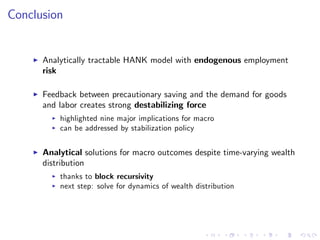
12. Budget constraint
ci,s + bi,s + xi,s = ni,s wi,s + (1 ni,s ) ϑ +
Rs 1
Πs
bi,s 1 +
(1 τi ) Rx,s
Πs
xi,s 1
Heterogeneous returns to equity due to individual-speci…c equity holding fee
τi 2 [0, 1]
I Benhabib, Bisin and Zhu (2011), Gabaix, Lasry, Lions and Moll (2016),
Fagereng, Guiso, Malacrino and Pistaferri (2016).
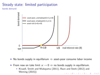
I special case: limited participation (τi 2 f0, 1g), Christiano, Eichenbaum
and Evans (1997)

13. Steady state: limited participation
equity demand
real return on equity (Rx)
equitydemand
0
Rx=1/β
supply
asset-poor, employed (τ=1,n=1)
asset-rich (τ=0,n=0)
asset-poor, unemployed (τ=1,n=0)
I Households with τi = 1 do not invest in equity and become
asset-poor
I Households with τi = 0 hold equity become asset-rich (assume rich
enough to drop out of labor force).

14. Steady state: limited participation
bonds demand
real interest rate (R)
bonddemand
0
R<1/β-ϗw 1/β
asset-poor, employed (τ=1,n=1)
asset-rich (τ=0,n=0)
asset-poor, unemployed (τ=1,n=0)
I No bonds supply in equilibrium ) asset-poor consume labor income
I From now on take limit { ! 0 ) no bonds supply in equilibrium.
I Krusell, Smith and Mukoyama (2011), Ravn and Sterk (2012) and
Werning (2015))

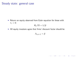
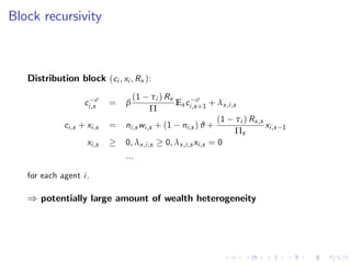
15. Steady state: general case
I Equity fee τi follows some distribution with support [0, 1].
I There is a threshold τ such that households with τi > τ do not
invest in equity and end up holding zero wealth in equilibrium
I ) ci,s = ni,s ws + (1 ni,s ) ϑ
I Let I = fi : τi > τ, ni,s = 1g be the set of households who never
invest in equity and are currently employed.
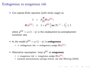
I Can show that, in equilibrium, these households are on their Euler
equation, i.e.
1 = β
R
Π
Es
ci,s
ci,s+1
σ
, i 2 I
β
R
Π
Es
ci,s
ci,s+1
σ
, i /2 I

16. Steady state: general case
I Return on equity observed from Euler equation for those with
τi = 0:
Rx /Π = 1/β
I All equity investors agree that …rms’discount factor should be
Λs,s+1 = β

17. Block recursivity
Macro block 1 (R, Π, η):
1 = β R
Π Θ(η) (EE)
1 γ + γmc(η) = φ(1 β)(Π 1)Π (PC)
R = maxfR Π/Π
δπ
(η/η)
δθ
1 α , 1g

18. Block recursivity
Macro block 1 (R, Π, η):
1 = β R
Π Θ(η) (EE)
1 γ + γmc(η) = φ(1 β)(Π 1)Π (PC)
R = maxfR Π/Π
δπ
(η/η)
δθ
1 α , 1g
where
Θ(η) 1 + ω (1 η)
h
(w (η) /ϑ) σ
1
i
1
mc(η)
w (η) +(κηα/(1 α)
λf )(1 β(1 ω)
1
β 1 + δ
η η, λf 0, λf η = 0

19. Block recursivity
Macro block 2 (n, k, y):
n = 1
ω
ω + ω (1 η)
1 = β 1 δ + µkµ 1
n1 µ
y = kµ
n1 µ

20. Block recursivity
Distribution block (ci , xi , Rx ):
c σ
i,s = β
(1 τi ) Rx
Π
Es c σ
i,s+1 + λx,i,s
ci,s + xi,s = ni,s wi,s + (1 ni,s ) ϑ +
(1 τi ) Rx,s
Πs
xi,s 1
xi,s 0, λx,i,s 0, λx,i,s xi,s = 0
...
for each agent i.
) potentially large amount of wealth heterogeneity

21. Endogenous vs exogenous risk
I Can express Euler equation (with sticky wage) as:
1 = β
R
Π
Θ(pEU
)
Θ(pEU
) 1 + pEU
h
(w/ϑ) σ
1
i
1
where pEU = ω (1 η) is the employment-to-unemployment
transition rate.
I In the model pEU = ω (1 η) is endogenous
I ) endogenous risk ) endogenous wedge Θ(pEU )
I Alternative assumption: treat pEU as exogenous.
I ) exogenous risk ) exogenous wedge Θ(pEU )
I constant precautionary savings motive, see also Werning (2015)

22. Steady states
3 cases:
I endogenous risk + ‡exible prices
I exogenous risk + sticky prices
I endogenous risk + sticky prices (baseline)

23. Steady states
I: intended steady state
II: liquidity trap
employment (n)
inflation(Π)
II
I
PC
EE (ZLB)
EE
ߜగ > 1, ߜఏ = 0
n=0
endogenous risk, flex price

24. Steady states
I: intended steady state
II: liquidity trap
employment (n)
inflation(Π)
I
II
EE
PC
EE (ZLB)
exogenous risk / full insurance, sticky price
n=0
ߜగ > 1, ߜఏ = 0

25. Implication 1: unemployment trap
I: intended steady state
II: liquidity trap
III: unemployment trap
inflation(Π)
employment (n)
EE
EE (ZLB)
PC
I
II
III
endogenous risk, sticky price
n=0
ߜగ > 1, ߜఏ = 0

26. Dynamics
I Consider local dynamics around intended steady state.
I For sake of simple formulas, assume δπ = 1
β > 1 (satis…es Taylor
principle), µ = 0 (no capital), and Λs,s+1 = β
I will all be relaxed
I Again, exploit block recursivity ) in…nite-dimensional,
time-varying wealth distribution in the background
I Log-linearize macro block

27. Dynamics
I Log-linearized Euler equation:
µbce,s + µβREsbce,s+1 = bRs Es bΠs+1 βR eΘEs bηs+1
| {z }
,
endogenous empl. risk
eΘ ωη (w (η) /ϑ) σ
1 0

28. Implication 2: breakdown Taylor principle
Equilibrium locally determinate if and only if:
φ
γ
|{z}
(
price rigidity
β2
R eΘ
| {z }
endog. risk
βδθ
1 α
| {z }
mon.policy
µβ 1 βR χ) <
κ
q
α
1 α
(1 β (1 ω)) +wχ
where χ
d ln w(η)
d ln η 0.
I Equilibrium always determinate if either φ = 0 (‡exible prices) or if
eΘ = 0 (full insurance or exogenous risk).
I More severe market incompleteness requires more aggressive
monetary policy to guarantee local determinacy around intended
steady state.

29. Implication 3: ampli…cation
I Solution for job …nding rate (sticky wage)
bηs = ΓηAs
Γη =
w κ
q β (1 ω) (1 ρ)
φγ 1β δθ
1 α ρβR eΘ + κ
q
α(1 ρβ(1 ω))
1 α
I Can show Γη > 0,
∂Γη
∂eΘ
> 0 and
∂Γη
∂eΘ∂φ
> 0
I ampli…cation due to interaction between endogenous risk and sticky
prices.
I lower productivity ) drop in vacancy posting ) lower goods
demand ) further drop in vacancy posting, etc.

30. Implication 3: ampli…cation
I Now include capital
I further ampli…cation or dampening?
I Also explore di¤erent assumptions on …rms’discount factors
I real interest rate vs subjective discount rate

31. Calibration
I Monthly model
Steady-state targets
u 0.05 unemployment rate
η 0.3 job …nding rate
κ
ψ3w 0.05 hiring cost as fraction of quarterly wage
6 avg. price duration (Calvo equivalent)
1 ϑ
w 0.15 income loss upon unemployment
Π 1 gross in‡ation rate
R12 1 0.03 annual net interest rate
k
12y 2 ratio capital to annual output

32. Calibration
Key parameter values
δπ 1.5 Taylor rule coe¢ cient in‡ation
δθ 0 Taylor rule coe¢ cient tightness
σ 2 coe¢ cient of risk aversion
χ 0 real wage ‡exibility parameter
δ 0.005 capital depreciation rate (monthly)
ω 0.02 job termination rate (monthly)
ρ 0.85 persistence technology shock
α 0.5 matching function elasticity
µ 0.3 production function elasticity

33. Implication 3: ampli…cation
Output response to TFP shock
0 10 20 30 40
0
1
2
3
4
5
A. WITHOUT CAPITAL
%
0 10 20 30 40
0
1
2
3
4
5
B. WITH CAPITAL
%
endogenous risk, sticky price
endogenous risk, flex price
exogenous risk, sticky price
TFP

34. Implication 4: nexus between real rate and tightness
bRr
s = (1 α) µχ + µχ + eΘ βRρ bθs
where bRr
s
bRs Es bΠs+1.
I Negative co-movement with exogenous risk or full insurance
(eΘ = 0). Positive co-movement between tightness and real
interest rate if eΘ large enough.
I Tight labor market ) low unemployment risk ) weak
precautionary savings motive ) high real interest rate

35. Implication 4: nexus between real rate and tightness
1990 1995 2000 2005 2010
-5
0
5
x 10
-3
realinterestrate(logpoints)
1990 1995 2000 2005 2010
-1.5
0
1.5
v-uratio(logpoints)
Real interest rate and labor market tightness (vacancy-unemployment ratio); deviations from trend. The real interest rate computed as the
Federal Funds rate minus a six-month moiving average of CPI in‡ation. Vacancies are measured as the composite Help Wanted index
from Barnichon (2010). Data series were logged and de-trended using a linear trend estimated over the period up to the end of 2007.

36. Implication 5: in‡ationary productivity shocks
Solution for in‡ation:
bΠs = ΓΠAs ,
where
ΓΠ =
β2
R eΘρ
βδθ
1 α
1 βρ
Γη
I Note: ΓΠ < 0 under complete markets (eΘ = 0).
I A positive productivity shock is in‡ationary if endogenous risk
channel su¢ ciently strong, i.e. if βR eΘρ > δθ
1 α
I Higher productivity ) higher employment ) weaker precautionary
savings motive ) higher goods demand ) in‡ationary pressure

37. Implication 5: in‡ationary productivity shocks
response to TFP0
0 5 10 15 20
-0.3
-0.2
-0.1
0
0.1
0.2
0.3
response to TFP1
0 5 10 15 20
-0.3
-0.2
-0.1
0
0.1
0.2
0.3
Notes: IRF of 400*log(cpit/cpit-1) to change in log TFP as estimated by Fernald (2016) using local projection. The sample starts in 1980
and we included 4 lags. TFP0 (TFP1) refers to Fernald estimate for Total Factor Productivity without (with) control for factor utilization.
Shaded areas denote error bands of two standard deviations.

38. Implication 6: sources of the ZLB
I If productivity shocks are in‡ationary, then a binding ZLB may arise
from a negative productivity shock, even if monetary policy
responds only to in‡ation.
I Log-linearized Euler equation:
µbce,s + µβREsbce,s+1 = bRs Es bΠs+1 βR eΘEs bηs+1
| {z }
,
endogenous empl. risk
I Wedge acts as endogenous discount factor shock, see also Werning
(2015)

39. Implication 7: missing de‡ation at the ZLB

40. Implication 7: missing de‡ation at the ZLB
Consider steady state with binding ZLB. Steady-state Euler equation:
1
Π
=
1
βΘ(η)
<
1
β
I Under complete markets (Θ(η) = 1) there must be de‡ation
(Π = β < 1)
I Under su¢ ciently strong increase in endogenous risk (Θ(η) > 1/β)
there is in‡ation at the ZLB (Π > 1)

41. Implication 8: supply shock paradox at the ZLB
I Endogenous risk can overturn the paradox that a positive
productivity shock creates an economic contraction at the ZLB
(Eggertsson, 2010):
I Assume ZLB persists with probability p.
I Slope (log-linearized) EE curve: d bΠs
dbηs
= µχ
p 1 βRp βR eΘ

42. Implication 8: supply shock paradox at the ZLB
inflationrate(Π)
job finding rate (η)
EE
PC’
B
exogenous risk
A
PC
inflationrate(Π)
job finding rate (η)
EE
PC’
B
endogenous risk
A
PC

43. Implication 9: asset pricing
I Two assets, both in zero net supply and available to everyone:
I zrisky
s which pays o¤ 1 + As+1 ρAs in period s + 1 (unit expected
payo¤).
I zriskless
s which pays o¤ 1 in period s + 1.
I Impose no-shortsale constraint on both assets (see also Krusell,
Mukoyama and Smith (2011)).

44. Implication 9: asset pricing
I Price di¤erence (based on log-linearized model) given by:
zriskless
s zrisky
s = βeΘΓησ2
A
I Positive risk premium due to endogenous risk (eΘ > 0).
I Monetary policy a¤ects risk premium via Γη

45. Conclusion
I Analytically tractable HANK model with endogenous employment
risk
I Feedback between precautionary saving and the demand for goods
and labor creates strong destabilizing force
I highlighted nine major implications for macro
I can be addressed by stabilization policy
I Analytical solutions for macro outcomes despite time-varying wealth
distribution
I thanks to block recursivity
I next step: solve for dynamics of wealth distribution

46. Appendix

47. Labor force participation in general case
I Given that households with τi = 0 withdraw from the labor force,
any household with τi > 0 will be in labor force. The Euler equation
for equity implies that:
c σ
i,s
Es c σ
i,s+1
= β
Rx
Π
(1 τi )
= (1 τi ) 1
which holds with strict inequality if τi > 0.
I Thus any household out of the labor force with τi > 0 will satisfy
ci,s+1
ci,s
< 1 i.e. have a strictly declining consumption pro…le. The
household eats into its savings.
I At some point, consumption of the household will be low that the
household will be back in the labor force.
I When back in the labor force, the precautionary motive kicks in,
which implies that Es ci,s+1 > ci,s .

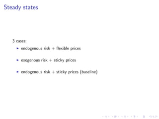
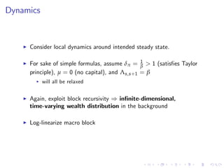
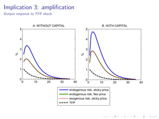
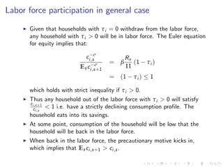
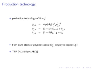
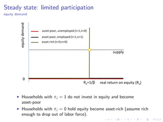
48. Role of …rms’discounting
Output response to TFP shock
0 10 20 30 40
0
1
2
3
4
5
A. WITHOUT CAPITAL
%
0 10 20 30 40
0
1
2
3
4
5
B. WITH CAPITAL
%
firms discount with subjective discount rate (1/)
firms discount with real interest rate (Es
[Rs
/s+1
])
TFP