Download to read offline

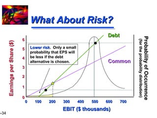
![16-5
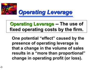
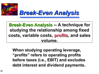
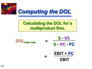
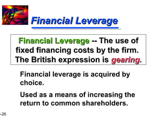
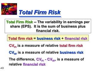
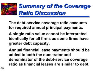
IImmppaacctt ooff OOppeerraattiinngg
LLeevveerraaggee oonn PPrrooffiittss
Now, subject each firm to a 5500%%
iinnccrreeaassee iinn ssaalleess for next year.
Which firm do you think will be more
““sseennssiittiivvee”” to the change in sales (i.e.,
show the largest percentage change in
operating profit, EBIT)?
[ ] FFiirrmm FF; [ ] FFiirrmm VV; [ ] FFiirrmm 22FF.](https://image.slidesharecdn.com/leverage-140910233646-phpapp01/85/Operating-and-Financial-Leverage-5-320.jpg)
![16-12
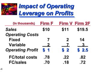
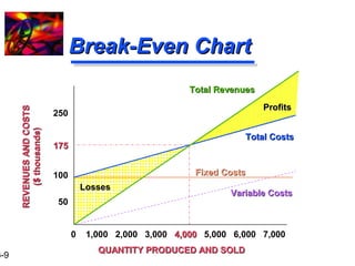
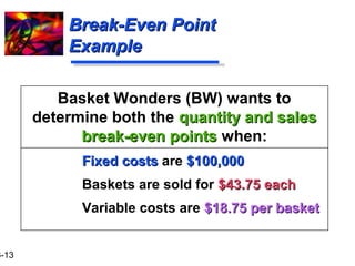
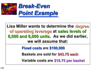
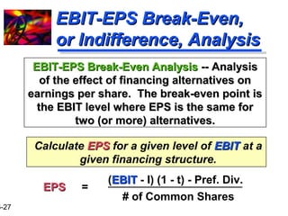
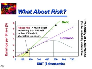
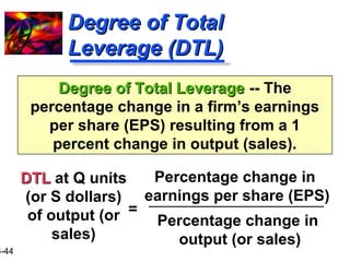
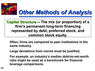
BBrreeaakk--EEvveenn ((SSaalleess)) PPooiinntt
How to find the sales break-even point:
SSBBEE = FFCC + (VVCCBBEE)
SSBBEE = FFCC + (QQBBEE )(VV)
or
SSBBEE
** = FFCC / [1 - (VVCC / S) ]
* Refer to text for derivation of the formula](https://image.slidesharecdn.com/leverage-140910233646-phpapp01/85/Operating-and-Financial-Leverage-12-320.jpg)

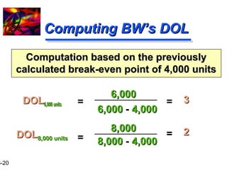
![16-37
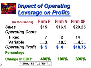
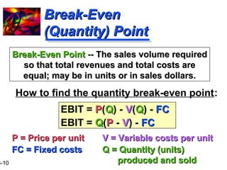
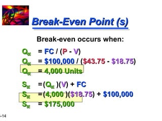
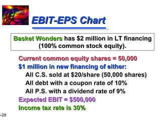
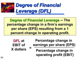
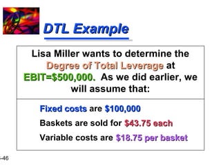
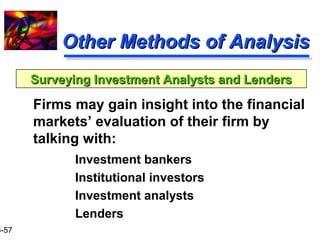
CCoommppuuttiinngg tthhee DDFFLL
DDFFLL EBIT of $X
CCaallccuullaattiinngg tthhee DDFFLL
= EBIT
EEBBIITT - II - [ PPDD / (1 - tt) ]
EEBBIITT == EEaarrnniinnggss bbeeffoorree iinntteerreesstt aanndd ttaaxxeess
II == IInntteerreesstt
PPDD == PPrreeffeerrrreedd ddiivviiddeennddss
tt == CCoorrppoorraattee ttaaxx rraattee](https://image.slidesharecdn.com/leverage-140910233646-phpapp01/85/Operating-and-Financial-Leverage-37-320.jpg)
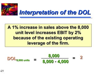
![16-38
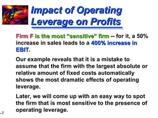
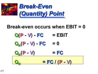
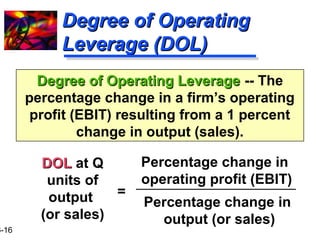
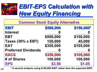
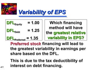
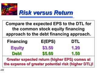
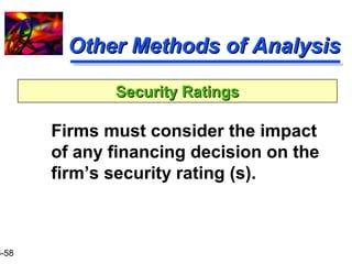
WWhhaatt iiss tthhee DDFFLL ffoorr EEaacchh
ooff tthhee FFiinnaanncciinngg CChhooiicceess??
CCaallccuullaattiinngg tthhee DDFFLL ffoorr NNEEWW eeqquuiittyy* aalltteerrnnaattiivvee
DDFFLL $$550000,,000000
= $500,000
$$550000,,000000 - 00 - [00 / (1 - 00)]
= 11..0000
* The calculation is based on the expected EBIT](https://image.slidesharecdn.com/leverage-140910233646-phpapp01/85/Operating-and-Financial-Leverage-38-320.jpg)
![16-39
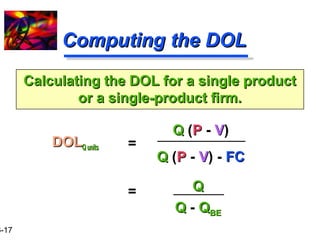
WWhhaatt iiss tthhee DDFFLL ffoorr EEaacchh
ooff tthhee FFiinnaanncciinngg CChhooiicceess??
CCaallccuullaattiinngg tthhee DDFFLL ffoorr NNEEWW ddeebbtt * aalltteerrnnaattiivvee
DDFFLL $$550000,,000000
= $500,000
{{ $$550000,,000000 - 110000,,000000
- [00 / (1 - 00)] }
= $$550000,,000000 / $400,000
= 11..2255
* The calculation is based on the expected EBIT](https://image.slidesharecdn.com/leverage-140910233646-phpapp01/85/Operating-and-Financial-Leverage-39-320.jpg)
![CCaallccuullaattiinngg tthhee DDFFLL ffoorr NNEEWW pprreeffeerrrreedd * aalltteerrnnaattiivvee
16-40
WWhhaatt iiss tthhee DDFFLL ffoorr EEaacchh
ooff tthhee FFiinnaanncciinngg CChhooiicceess??
DDFFLL $$550000,,000000
= $500,000
{{ $$550000,,000000 - 00
- [9900,,000000 / (1 - ..3300)] }
= $$550000,,000000 / $400,000
= 11..3355
* The calculation is based on the expected EBIT](https://image.slidesharecdn.com/leverage-140910233646-phpapp01/85/Operating-and-Financial-Leverage-40-320.jpg)

![16-45
CCoommppuuttiinngg tthhee DDTTLL
DDTTLL QQ uunniittss ((oorr SS ddoollllaarrss)) = ( DDOOLL QQ uunniittss ((oorr SS ddoollllaarrss)) )
DDTTLL S dollars
of sales
x ( DDFFLL EEBBIITT ooff XX ddoollllaarrss )
= EBIT + FC
EEBBIITT - II - [ PPDD / (1 - tt) ]
DDTTLL Q units
QQ (PP -- VV)
QQ (PP -- VV) - FC - II - [ PPDD / (1 - tt) ]
=](https://image.slidesharecdn.com/leverage-140910233646-phpapp01/85/Operating-and-Financial-Leverage-45-320.jpg)
![16-47
CCoommppuuttiinngg tthhee DDTTLL
ffoorr AAllll--EEqquuiittyy FFiinnaanncciinngg
DDTTLLSS ddoollllaarrss = (DDOOLL SS ddoollllaarrss) x (DDFFLLEEBBIITT ooff $$SS )
DDTTLLSS ddoollllaarrss = (11..22 ) x ( 11..00* ) = 11..2200
DDTTLL S dollars
of sales
=
$$550000,,000000 + $100,000
$$550000,,000000 - 00 - [ 00 / (1 - ..33) ]
= 11..2200
*Note: No financial leverage.](https://image.slidesharecdn.com/leverage-140910233646-phpapp01/85/Operating-and-Financial-Leverage-47-320.jpg)
![16-48
CCoommppuuttiinngg tthhee DDTTLL
ffoorr DDeebbtt FFiinnaanncciinngg
DDTTLLSS ddoollllaarrss = (DDOOLL SS ddoollllaarrss) x (DDFFLLEEBBIITT ooff $$SS )
DDTTLLSS ddoollllaarrss = (11..22 ) x ( 11..2255* ) = 11..5500
DDTTLL S dollars
of sales
=
$$550000,,000000 + $100,000
{ $$550000,,000000 - $$110000,,000000
- [ 00 / (1 - ..33) ] }
= 11..5500
*Note: Calculated on Slide 39.](https://image.slidesharecdn.com/leverage-140910233646-phpapp01/85/Operating-and-Financial-Leverage-48-320.jpg)
![16-52
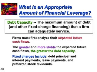
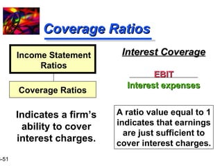
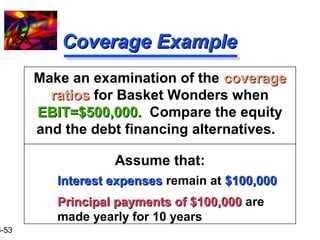
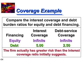
CCoovveerraaggee RRaattiiooss
DDeebbtt--sseerrvviiccee CCoovveerraaggee
EEBBIITT
{ IInntteerreesstt eexxppeennsseess +
[PPrriinncciippaall ppaayymmeennttss // ((11--tt)) ] }
Income Statement
Ratios
Coverage Ratios
Indicates a firm’s
ability to cover
interest expenses and
principal payments.
Allows us to examine the
ability of the firm to meet
all of its debt payments.
Failure to make principal
payments is also default.](https://image.slidesharecdn.com/leverage-140910233646-phpapp01/85/Operating-and-Financial-Leverage-52-320.jpg)

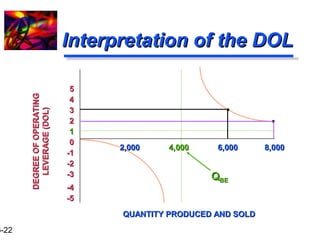
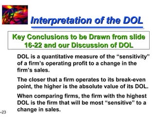
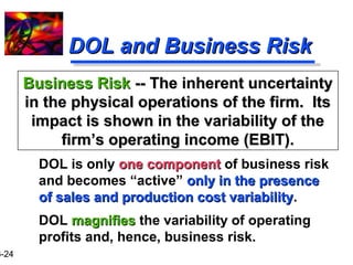
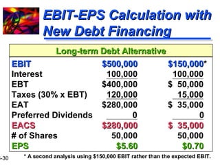
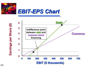
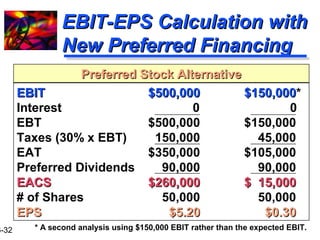
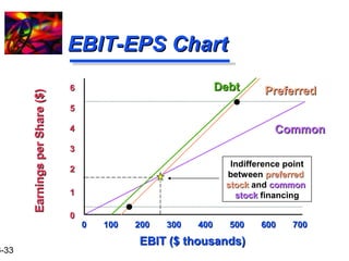
This document discusses operating leverage and financial leverage. It defines operating leverage as the use of fixed operating costs by a firm and financial leverage as the use of fixed financing costs. It then provides examples to illustrate how operating leverage can impact a firm's profits and how to calculate measures of operating leverage like the break-even point and degree of operating leverage (DOL). The DOL measures the percentage change in operating profit from a 1% change in sales. Firms closer to the break-even point have a higher DOL and are more sensitive to sales changes. Financial leverage is used to increase returns for common shareholders but also increases business risk.


![[wacc] weighted average cost of capital](https://cdn.slidesharecdn.com/ss_thumbnails/anuragmathur-210703072911-thumbnail.jpg?width=640&height=640&fit=bounds)