This document contains lecture notes on the design and analysis of algorithms. It covers topics like algorithm definition, complexity analysis, divide and conquer algorithms, greedy algorithms, dynamic programming, and NP-complete problems. The notes provide examples of algorithms like selection sort, towers of Hanoi, and generating permutations. Pseudocode is used to describe algorithms precisely yet readably.


![Design and Analysis of Algorithms
Dept. of CSE, SWEC, Hyderaba. Page 4
If <condition> then <statement>
If <condition> then <statement-1>
Else <statement-1>
Case statement:
Case
{
: <condition-1> : <statement-1>
.
.
.
: <condition-n> : <statement-n>
: else : <statement-n+1>
}
9. Input and output are done using the instructions read & write.
10. There is only one type of procedure:
Algorithm, the heading takes the form,
Algorithm Name (Parameter lists)
As an example, the following algorithm fields & returns the maximum of ‘n’
given
numbers:
1. algorithm Max(A,n)
2. // A is an array of size n
3. {
4. Result := A[1];
5. for I:= 2 to n do
6. if A[I] > Result then
7. Result :=A[I];
8. return Result;
9. }](https://image.slidesharecdn.com/daanotes-231027021902-07b9e3d5/85/DAA-Notes-pdf-6-320.jpg)
![Design and Analysis of Algorithms
Dept. of CSE, SWEC, Hyderaba. Page 5
In this algorithm (named Max), A & n are procedure parameters. Result & I are
Local variables.
Next we present 2 examples to illustrate the process of translation problem into
an
algorithm.
Selection Sort:
• Suppose we Must devise an algorithm that sorts a collection of n>=1
elements of arbitrary type.
• A Simple solution given by the following.
• ( From those elements that are currently unsorted ,find the smallest & place
it next in the sorted list.)
Algorithm:
1. For i:= 1 to n do
2. {
3. Examine a[I] to a[n] and suppose the smallest element is at a[j];
4. Interchange a[I] and a[j];
5. }
Finding the smallest element (sat a[j]) and interchanging it with a[ i ]
• We can solve the latter problem using the code,
t := a[i];
a[i]:=a[j];
a[j]:=t;
• The first subtask can be solved by assuming the minimum is a[ I ];checking
a[I] with a[I+1],a[I+2]…….,and whenever a smaller element is found,
regarding it as the new minimum. a[n] is compared with the current
minimum.
• Putting all these observations together, we get the algorithm Selection sort.](https://image.slidesharecdn.com/daanotes-231027021902-07b9e3d5/85/DAA-Notes-pdf-7-320.jpg)
![Design and Analysis of Algorithms
Dept. of CSE, SWEC, Hyderaba. Page 6
Theorem:
Algorithm selection sort(a,n) correctly sorts a set of n>=1 elements .The result
remains is a a[1:n] such that a[1] <= a[2] ….<=a[n].
Selection Sort:
Selection Sort begins by finding the least element in the list. This element is moved to
the front. Then the least element among the remaining element is found out and put into
second position. This procedure is repeated till the entire list has been studied.
Example:
LIST L = 3,5,4,1,2
1 is selected , 1,5,4,3,2 2 is selected,
1,2,4,3,5
3 is selected, 1,2,3,4,5
4 is selected, 1,2,3,4,5
Proof:
• We first note that any I, say I=q, following the execution of lines 6 to 9,it
is the case that a[q] Þ a[r],q<r<=n.
• Also observe that when ‘i’ becomes greater than q, a[1:q] is unchanged.
Hence, following the last execution of these lines (i.e. I=n).We have a[1]
<= a[2] <=……a[n].
• We observe this point that the upper limit of the for loop in the line 4 can
be changed to n-1 without damaging the correctness of the algorithm.
Algorithm:
1. Algorithm selection sort (a,n)
2. // Sort the array a[1:n] into non-decreasing order.
3.{
4. for I:=1 to n do
5. {
6. j:=I;
7. for k:=i+1 to n do
8. if (a[k]<a[j])](https://image.slidesharecdn.com/daanotes-231027021902-07b9e3d5/85/DAA-Notes-pdf-8-320.jpg)
![Design and Analysis of Algorithms
Dept. of CSE, SWEC, Hyderaba. Page 7
9. t:=a[I];
10. a[I]:=a[j];
11. a[j]:=t;
12. }
13. }
Recursive Algorithms:
• A Recursive function is a function that is defined in terms of itself.
• Similarly, an algorithm is said to be recursive if the same algorithm is invoked in
the body.
• An algorithm that calls itself is Direct Recursive.
• Algorithm ‘A’ is said to be Indirect Recursive if it calls another algorithm which
in turns calls ‘A’.
• The Recursive mechanism, are externally powerful, but even more importantly,
many times they can express an otherwise complex process very clearly. Or these
reasons we introduce recursion here.
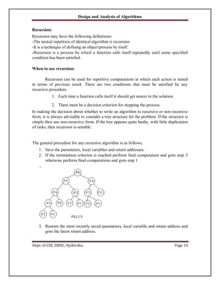
• The following 2 examples show how to develop a recursive algorithms.
In the first, we consider the Towers of Hanoi problem, and in
the second, we generate all possible permutations of a list of
characters.
Tower A Tower B Tower C
• It is Fashioned after the ancient tower of Brahma ritual.
1. Towers of Hanoi:
.
.
.](https://image.slidesharecdn.com/daanotes-231027021902-07b9e3d5/85/DAA-Notes-pdf-9-320.jpg)


![Design and Analysis of Algorithms
Dept. of CSE, SWEC, Hyderaba. Page 10
1.A fixed part that is independent of the characteristics (eg:number,size)of the inputs
and outputs.
The part typically includes the instruction space (ie. Space for the code), space
for simple variable and fixed-size component variables (also called aggregate) space
for constants, and so on.
2. A variable part that consists of the space needed by component variables whose
size is dependent on the particular problem instance being solved, the space
needed by referenced variables (to the extent that is depends on instance
characteristics), and the recursion stack space.
• The space requirement s(p) of any algorithm p may therefore be
written as,
S(P) = c+ Sp(Instance characteristics)
Where ‘c’ is a constant.
Example 2:
Algorithm sum(a,n)
{
s=0.0;
for I=1 to n do s=
s+a[I];
return s;
}
• The problem instances for this algorithm are characterized by n,the
number of elements to be summed. The space needed d by ‘n’ is one
word, since it is of type integer.
• The space needed by ‘a’a is the space needed by variables of tyepe
array of floating point numbers.
• This is atleast ‘n’ words, since ‘a’ must be large enough to hold the ‘n’
elements to be summed.
• So,we obtain Ssum(n)>=(n+s)
[ n for a[],one each for n,I a& s]
Time Complexity:
The time T(p) taken by a program P is the sum of the compile time and the
run time(execution time)](https://image.slidesharecdn.com/daanotes-231027021902-07b9e3d5/85/DAA-Notes-pdf-12-320.jpg)
![Design and Analysis of Algorithms
Dept. of CSE, SWEC, Hyderaba. Page 11
The compile time does not depend on the instance characteristics. Also we
may assume that a compiled program will be run several times without
recompilation .This rum time is denoted by tp(instance characteristics).
The number of steps any problem statemn t is assigned depends on the kind
of statement.
For example, comments 0 steps.
Assignment statements 1 steps.
[Which does not involve any calls to other algorithms]
Interactive statement such as for, while & repeat-until Control part of the statement.
1. We introduce a variable, count into the program statement to increment count with
initial value 0.Statement to increment count by the appropriate amount are
introduced into the program.
This is done so that each time a statement in the original program is executes
count is incremented by the step count of that statement.
Algorithm:
Algorithm sum(a,n)
{ s= 0.0; count
=
count+1;
for I=1 to
n do
{
count =count+1;
s=s+a[I];
count=count+1;
} count=count+1;
count=count+1; return s;
}
If the count is zero to start with, then it will be 2n+3 on termination. So each
invocation of sum execute a total of 2n+3 steps.](https://image.slidesharecdn.com/daanotes-231027021902-07b9e3d5/85/DAA-Notes-pdf-13-320.jpg)
![Design and Analysis of Algorithms
Dept. of CSE, SWEC, Hyderaba. Page 12
2. The second method to determine the step count of an algorithm is to build
a table in which we list the total number of steps contributes by each
statement.
First determine the number of steps per execution (s/e) of the statement and the
total number of times (ie., frequency) each statement is executed.
By combining these two quantities, the total contribution of all statements, the
step count for the entire algorithm is obtained.
Statement S/e Frequency Total
1. Algorithm Sum(a,n)
2.{
3. S=0.0;
4. for I=1 to n do
5. s=s+a[I];
6. return s;
7. }
0
0
1
1
1
1
0
-
-
1
n+1
n
1
-
0
0
1
n+1
n 1
0
Total 2n+3
AVERAGE –CASE ANALYSIS
• Most of the time, average-case analysis are performed under the more or less
realistic assumption that all instances of any given size are equally likely.
• For sorting problems, it is simple to assume also that all the elements to be
sorted are distinct.
• Suppose we have ‘n’ distinct elements to sort by insertion and all n!
permutation of these elements are equally likely.
• To determine the time taken on a average by the algorithm ,we could add the
times required to sort each of the possible permutations ,and then divide by n!
the answer thus obtained.
• An alternative approach, easier in this case is to analyze directly the time
required by the algorithm, reasoning probabilistically as we proceed.
• For any I,2≤ I≤n, consider the sub array, T[1….i].](https://image.slidesharecdn.com/daanotes-231027021902-07b9e3d5/85/DAA-Notes-pdf-14-320.jpg)
![Design and Analysis of Algorithms
Dept. of CSE, SWEC, Hyderaba. Page 13
• The partial rank of T[I] is defined as the position it would occupy if the sub
array were sorted.
• For Example, the partial rank of T[4] in [3,6,2,5,1,7,4] in 3 because T[1….4]
once sorted is [2,3,5,6].
• Clearly the partial rank of T[I] does not depend on the order of the element in
• Sub array T[1…I-1].
Analysis
Best case:
This analysis constrains on the input, other than size. Resulting in the fasters possible run
time
Worst case:
This analysis constrains on the input, other than size. Resulting in the fasters
possible run time
Average case:
This type of analysis results in average running time over every type of input.
Complexity:
Complexity refers to the rate at which the storage time grows as a function of
the problem size
Asymptotic analysis:
Expressing the complexity in term of its relationship to know function.
This type analysis is called asymptotic analysis.
Asymptotic notation:
Big ‘oh’: the function f(n)=O(g(n)) iff there exist positive constants c and no such that
f(n)≤c*g(n) for all n, n ≥ no.
Omega: the function f(n)=Ω(g(n)) iff there exist positive constants c and no such that f(n)
≥ c*g(n) for all n, n ≥ no.
Theta: the function f(n)=ө(g(n)) iff there exist positive constants c1,c2 and no such that
c1 g(n) ≤ f(n) ≤ c2 g(n) for all n, n ≥ no.](https://image.slidesharecdn.com/daanotes-231027021902-07b9e3d5/85/DAA-Notes-pdf-15-320.jpg)


![Design and Analysis of Algorithms
Dept. of CSE, SWEC, Hyderaba. Page 18
• The pattern is now obvious.
T(2k
) = 3k
20
+ 3k-1
21
+ 3k-2
22
+…+31
2k-1
+ 30
2k
.
= ∑ 3k-i
2i
= 3k
∑ (2/3)i
= 3k
* [(1 – (2/3)k + 1
) / (1 – (2/3)]
= 3k+1
– 2k+1
Proposition: (Geometric Series)
Let Sn be the sum of the first n terms of the geometric series a, ar,
ar2
….Then Sn = a(1-rn
)/(1-r), except in the special case when r = 1; when Sn =
an.
= 3k
* [ (1 – (2/3) k+1
) / (1 – (2/3))]
= 3k
* [((3 k+1
– 2 k+1
)/ 3 k+1
) / ((3 – 2) / 3)]
3 k+1
– 2k+1
3
= 3k
* -----------------
* ---- 3
k+1
1
3 k+1
– 2k+
1
= 3k
* ---------------
-- 3k+1-1
= 3k+1
– 2k+1
* It is easy to check this formula against our earlier tabulation.
EG : 2](https://image.slidesharecdn.com/daanotes-231027021902-07b9e3d5/85/DAA-Notes-pdf-20-320.jpg)


![Design and Analysis of Algorithms
Dept. of CSE, SWEC, Hyderaba. Page 22
when n=0, f0 = C1 + C2 = 0
when n=1, f1 = C1r1 + C2r2 = 1
C1 + C2 = 0 (1)
C1r1 + C2r2 = 1 (2)
From equation (1)
C1 = -C2
Substitute C1 in equation(2)
-C2r1 + C2r2 = 1
C2[r2 – r1] = 1
Substitute r1 and r2 values
1 - √5 1 - √5
C2 --------- - --------- = 1
2 2
1 – √5 – 1 – √5
C2 --------------------- = 1
2
-C2 * 2√5
-------------- = 1
2
– √5C2 = 1
C1 = 1/√5 C2 = -1/√5
Thus,
1 1 + √5 n
-1 1
- √5 n
fn = ---- --------- +
---- -------- √5 2
√5 2
1 1 + √5 n
1 – √5 n
= ---- --------- - ---------
√5 2 2](https://image.slidesharecdn.com/daanotes-231027021902-07b9e3d5/85/DAA-Notes-pdf-24-320.jpg)
![Design and Analysis of Algorithms
Dept. of CSE, SWEC, Hyderaba. Page 24
(2) * 2 2C1 + 2C2 = 2t0
2C1 + 3C2 = (3 + 2t0)
-------------------------------
-C2 = -3
C2 = 3
Sub C2 = 3 in eqn (2)
C1 + C2 = t0
C1 + 3 = t0
C1 = t0 – 3
Therefore tn = (t0-3)2n
+ 3. 3n
= Max[O[(t0 – 3) 2n
], O[3.3n
]]
= Max[O(2n
), O(3n
)] constants
= O[3n
]
Example :(2)
tn – 2t n-1 = (n + 5)3n
, n ≥ 1 (A)
This is Inhomogeneous
In this case, b=3, p(n) = n+5, degree = 1
So, the characteristic polynomial is,
(x-2)(x-3)2
= 0
The roots are,
r1 = 2, r2 = 3, r3 = 3
The general equation, tn
= C1r1
n
+ C2r2
n
+ C3nr3
n
(1)
when n=0, t0 = C1 + C2 (2)
when n=1, t1 = 2C1 + 3C2 + 3C3 (3)
substituting n=1 in eqn(A),
t1 –
2t0 = 6 . 3](https://image.slidesharecdn.com/daanotes-231027021902-07b9e3d5/85/DAA-Notes-pdf-26-320.jpg)
![Design and Analysis of Algorithms
Dept. of CSE, SWEC, Hyderaba. Page 25
t1 – 2t0 = 18
t1 = 18 + 2t0
substituting t1 value in eqn(3)
2C1 + 3C2 + 3C3 = 18 + 2t0
(4) C1 + C2 + = t0
(2)
Sub. n=2 in eqn(1)
4C1 + 9C2 + 18C3 = t2 (5)
sub n=2 in eqn (A)
t2 – 2t1 = 7. 9
t2 = 63 + 2t1
= 63 + 2[18 +
2t0] t2 = 63 +
36 +4t0 t2 =
99 +4t0
sub. t2 value in eqn(3), 4C1
+9C2 + 18C3 = 99 + 4t0
(5)
solve eqn (2),(4) & (5)
n=0, C1 + C2 = t0
(2) n=1, 2C1 + 3C2 + 3C3 = 18 +
2t0 (4) n=2, 4C1 + 9C2 + 18C3
= 99 + 4t0 (5)
(4) * 6 12C1 + 18C2 +18C3 = 108 + 2t0 (4)
(5) 4C1 + 9C2 + 18C3 = 99 + 4t0 (5)
------------------------------------------------
8C1 + 9C2 = 9 + 8t0 (6)
(2) * 8 8C1 + 8C2 = 8t0 (2)
(6) 8C1 + 9C2 = 9 +8t0 (6)
--------------------------
-C2 = -9
C2 = 9](https://image.slidesharecdn.com/daanotes-231027021902-07b9e3d5/85/DAA-Notes-pdf-27-320.jpg)
![Design and Analysis of Algorithms
Dept. of CSE, SWEC, Hyderaba. Page 26
Sub, C2 = 9 in eqn(2)
C1 + C2 = t0
C1 + 9 = t0
C1 = t0-9
Sub C1 & C2 in eqn (4)
2C1 + 3C2 + 3C3 = 18 + 2t0
2(t0-9) + 3(9) + 3C3 = 18 + 2t0
2t0 – 18 + 27 + 3C3 = 18 + 2t0
2t0 + 9 + 3C3 = 18 + 2t0
3C3 = 18 – 9 + 2t0 – 2t0
3C3 = 9
C3 = 9/3
C3 = 3
Sub. C1, C2, C3, r1, r2, r3 values in
eqn (1) tn = C12n
+ C23n
+
C3.n.3n
= (t0 – 9)2n
+ 9.3n
+ 3.n.3n
= Max[O[(t0-9),2n
], O[9.3n
], O[3.n.3n
]]
= Max[O(2n
), O(3n
),
O(n3n
)] tn = O[n3n
]
Example: (3)
Consider the recurrence,
1
if n=0 tn =
4t n-1 – 2n
otherwise
tn – 4t n-1 = -2n (A)
In this case , c=2, p(n) = -1, degree =0
(x-4)(x-2) = 0
The roots are, r1 = 4, r2 = 2](https://image.slidesharecdn.com/daanotes-231027021902-07b9e3d5/85/DAA-Notes-pdf-28-320.jpg)
![Design and Analysis of Algorithms
Dept. of CSE, SWEC, Hyderaba. Page 27
The general
solution ,
tn = C1r1
n
+ C2r2
n
tn = C14n
+ C22n
(1)
when n=0, in (1) C1 + C2 = 1 (2)
when n=1, in (1) 4C1 + 2C2 = t1 (3)
sub n=1 in (A),
tn – 4t n-1 = -2n
t1 – 4t0 = -2 t1 =
4t0 – 2 [since t0 = 1]
t1 = 2
sub t1 value in eqn (3)
4C1 + 2C2 = 4t0 – 2 (3)
(2) * 4 4C1 + 4C2 = 4
----------------------------
-2C2 = 4t0 - 6
= 4(1) - 6
= -2
C2 = 1
-2C2 = 4t0 - 6
2C2 = 6 – 4t0
C2 = 3 – 2t0
3 – 2(1) = 1
C2 = 1
Sub. C2 value in eqn(2),
C1 + C2 = 1
C1 + (3-2t0) = 1
C1 + 3 – 2t0 = 1
C1 = 1 – 3 + 2t0
C1 = 2t0 - 2
= 2(1) –
2 = 0 C1 = 0](https://image.slidesharecdn.com/daanotes-231027021902-07b9e3d5/85/DAA-Notes-pdf-29-320.jpg)
![Design and Analysis of Algorithms
Dept. of CSE, SWEC, Hyderaba. Page 28
Sub C1 & C2 value in
eqn (1) tn = C14n
+
C22n
= Max[O(2t0 – 2).4n
, O(3 – 2t0).2n
]
= Max[O(2n
)]
tn = O(2n
)
Example : (4)
0
if n=0 tn =
2t n-1 + n +2n
otherwise
tn – 2t n-1 = n + 2n
(A)
There are two polynomials.
For n; b=1, p(n), degree = 1
For 2n; b=2, p(n) = 1, degree =0
The characteristic polynomial is,
(x-2)(x-1)2
(x-2) = 0
The roots are, r1 = 2, r2 = 2, r3 = 1,
r4 = 1. So, the general solution,
tn = C1r1
n
+ C2nr2
n
+ C3r3
n
+ C4 n
r4
n
sub r1, r2, r3 in the above eqn
tn = 2n
C1 + 2n
C2 n + C3 . 1n
+ C4 .n.1n
(1)
sub. n=0 C1 + C3 = 0
(2) sub. n=1 2C1 + 2C2 + C3 + C4 = t1
(3)
sub. n=1 in eqn (A)
tn -2t n-1 = n + 2n
t1 – 2t0 = 1 + 2 t1](https://image.slidesharecdn.com/daanotes-231027021902-07b9e3d5/85/DAA-Notes-pdf-30-320.jpg)
![Design and Analysis of Algorithms
Dept. of CSE, SWEC, Hyderaba. Page 29
– 2t0 = 3 t1
= 3 [since t0 = 0]
sub. n=2 in eqn (1)
22
C1 + 2. 22
.C2 + C3 + 2.C4 = t2
4C1 + 8C2 + C3 + 2C4 = t2
sub n=2 in eqn (A)
t2 – 2t1 = 2 + 22
t2 – 2t1 =
2 + 4 t2
– 2t1 = 6
t2 = 6 + 2t1
t2 = 6 + 2.3
t2 = 6 + 6
t2 = 12
4C1 + 8C2 + C3 + 2C4 = 12 (4)
sub n=3 in eqn (!)
23
C1 + 3.23
.C2 + C3 + 3C4 = t3
3C1 + 24C2 + C3 + 3C4 = t3
sub n=3 in eqn (A)
t3 – 2t2 =
3 + 23
t3
– 2t2 = 3 + 8
t3 – 2(12) =
11 t3 – 24
= 11
t3 = 11 + 24
t3 = 35
8C1 + 24C2 + C3 + 3C4 = 35 (5)
n=0, solve; C1 + C3 = 0 (2)
n=1,(2), (3), (4)&(5) 2C1 + 2C2 + C3 + C4 = 3 (3)
n=2, 4C1 + 8C2 + C3 + 2C4 = 12 (4)
n=3, 8C1 + 24C2 + C3 + 3C4 = 35 (5)](https://image.slidesharecdn.com/daanotes-231027021902-07b9e3d5/85/DAA-Notes-pdf-31-320.jpg)

![Design and Analysis of Algorithms
Dept. of CSE, SWEC, Hyderaba. Page 31
* This is achieved by introducing new recurrence ti, define by ti = T(2i
) *
This transformation is useful because n/2 becomes (2i
)/2 = 2 i-1
* In other words, our original recurrence in which T(n) is defined as a
function of T(n/2) given way to one in which ti is defined as a
function of t i-1, precisely the type of recurrence we have learned to
solve.
ti = T(2i
) = 3T(2 i-
1
) + 2i
ti = 3t i-1 +
2i
ti – 3t i-1 = 2i
(A)
In this case,
b = 2, p(n) = 1, degree = 0
So, the characteristic equation,
(x – 3)(x – 2) = 0
The roots are, r1 = 3, r2 = 2.
The general equation,
tn = C1 r1
i
+ C2 r2
i
sub. r1 & r2: tn = 3n
C1 +
C2 2n
tn =
C1 3i
+ C2 2i
We use the fact that, T(2i
) = ti & thus T(n) = tlogn when n= 2i
to obtain,
T(n) = C1. 3 log
2
n
+ C2. 2log
2
n
T(n) = C1 . nlog
2
3
+ C2.n [i = logn]
When ‘n’ is a power of 2, which is sufficient to conclude that,
T(n) = O(n log3
) ‘n’ is a power of 2
Example: (2)
Consider the recurrence,
T(n) = 4T(n/2) + n2
(A)
Where ‘n’ is a power of 2, n ≥ 2.](https://image.slidesharecdn.com/daanotes-231027021902-07b9e3d5/85/DAA-Notes-pdf-33-320.jpg)
![Design and Analysis of Algorithms
Dept. of CSE, SWEC, Hyderaba. Page 32
ti = T(2i
) = 4T(2 i-1
) + (2i
)2
ti = 4t i-1 + 4i
ti – 4t i-1 = 4i
In this eqn,
b = 4, P(n) = 1, degree = 0
The characteristic polynomial,
(x – 4)(x – 4) = 0
The roots are, r1 = 4, r2 = 4.
So, the general equation, ti = C14i
+ C24i
.i [since i = logn]
= C1 4 log n
+ C2. 4 logn
. logn [since 2i
= n]
= C1 . n log 4 + C2. n log4.nlog1
T(n) = O(n log4
) ‘n’ is the power of 2.
EXAMPLE : 3
T(n) = 2T(n/2) + n logn
When ‘n’ is a power of 2, n ≥ 2
ti = T(2i
) = 2T(2i
/2) + 2i
.i [since 2i
= n; i =logn] ti
– 2t i-1 = i. 2i
In this case,
b = 2, P(n) = i, degree = 1
(x – 2)(x – 2)2
= 0
The roots are, r1 = 2, r2 = 2, r3 = 2
The general solution is,
tn = C12i
+ C2. 2i
. i + C3. i2
.](https://image.slidesharecdn.com/daanotes-231027021902-07b9e3d5/85/DAA-Notes-pdf-34-320.jpg)


![Design and Analysis of Algorithms
Dept. of CSE, SWEC, Hyderaba. Page 38
approximate mid entry is located and its key value is examined. If the mid value is greater
than X, then the list is chopped off at the (mid-1)th
location. Now the list gets reduced to
half the original list. The middle entry of the left-reduced list is examined in a similar
manner. This procedure is repeated until the item is found or the list has no more
elements. On the other hand, if the mid value is lesser than X, then the list is chopped off
at (mid+1)th
location. The middle entry of the right-reduced list is examined and the
procedure is continued until desired key is found or the search interval is exhausted.
The algorithm for binary search is as follows,
Algorithm : binary search
Input : A, vector of n elements
K, search element
Output : low –index of k
Method : low=1,high=n
While(low<=high-1)
{
mid=(low+high)/2
if(k<a[mid])
high=mid
else
low=mid
if end
}
if(k=A[low])
{
write("search successful")
write(k is at location low)
exit(); } else write
(search
unsuccessful);
if end;
algorithm
ends.
SORTING
One of the major applications in computer science is the sorting of information in
a table. Sorting algorithms arrange items in a set according to a predefined ordering
relation. The most common types of data are string information and numerical](https://image.slidesharecdn.com/daanotes-231027021902-07b9e3d5/85/DAA-Notes-pdf-40-320.jpg)
![Design and Analysis of Algorithms
Dept. of CSE, SWEC, Hyderaba. Page 39
information. The ordering relation for numeric data simply involves arranging items in
sequence from smallest to largest and from largest to smallest, which is called ascending
and descending order respectively.
The items in a set arranged in non-decreasing order are {7,11,13,16,16,19,23}. The items
in a set arranged in descending order is of the form {23,19,16,16,13,11,7}
Similarly for string information, {a, abacus, above, be, become, beyond}is in ascending
order and { beyond, become, be, above, abacus, a}is in descending order.
There are numerous methods available for sorting information. But, not even one of them
is best for all applications. Performance of the methods depends on parameters like, size
of the data set, degree of relative order already present in the data etc.
Selection sort :
The idea in selection sort is to find the smallest value and place it in an order, then
find the next smallest and place in the right order. This process is continued till the entire
table is sorted.
Consider the unsorted
array, a[1] a[2] a[8]
20 35 18 8 14 41 3 39
The resulting array should be
a[1] a[2] a[8]
3 8 14 18 20 35 39 41
One way to sort the unsorted array would be to perform the following steps:
• Find the smallest element in the unsorted array
• Place the smallest element in position of a[1]
i.e., the smallest element in the unsorted array is 3 so exchange the values of a[1]
and a[7]. The array now becomes,
a[1] a[2] a[8]
3 35 18 8 14 41 20 39](https://image.slidesharecdn.com/daanotes-231027021902-07b9e3d5/85/DAA-Notes-pdf-41-320.jpg)
![Design and Analysis of Algorithms
Dept. of CSE, SWEC, Hyderaba. Page 40
Now find the smallest from a[2] to a[8] , i.e., 8 so exchange the values of a[2] and
a[4] which results with the array shown below,
a[1] a[2] a[8]
3 8 18 35 14 41 20 39
Repeat this process until the entire array is sorted. The changes undergone by the array is
shown in fig 2.2.The number of moves with this technique is always of the order O(n).
Bubble sort:
Bubble Sort is an elementary sorting algorithm. It works by repeatedly exchanging
adjacent elements, if necessary. When no exchanges are required, the file is sorted.
BUBBLESORT (A)
for i ← 1 to length [A] do
for j ← length [A] downto i+1 do
If A[A]
Exchange A[j] ↔ A[j-1]
< A[j-1] then
Here the number
1 + 2 + 3 + . . . + (n-1) = n(n-1)/2 = O(n2
)
of comparison made
Another well-known sorting method is bubble sort. It differs from the selection
sort in that instead of finding the smallest record and then performing an interchange two
records are interchanged immediately upon discovering that they are of out of order.](https://image.slidesharecdn.com/daanotes-231027021902-07b9e3d5/85/DAA-Notes-pdf-42-320.jpg)
![Design and Analysis of Algorithms
Dept. of CSE, SWEC, Hyderaba. Page 41
When this approach is used there are at most n-1 passes required. During the first pass
k1and k2 are compared, and if they are out of order, then records R1 AND R2 are
interchanged; this process is repeated for records R2 and R3, R3 and R4 and so on .this
method will cause with small keys to bubble up. After the first pass the record with the
largest key will be in the nth position. On each successive pass, the records with the next
largest key will be placed in the position n-1, n-2 …2 respectively, thereby resulting in a
sorted table.
After each pass through the table, a check can be made to determine whether any
interchanges were made during that pass. If no interchanges occurred then the table must
be sorted and no further passes are required.
Insertion sort :
Insertion sort is a straight forward method that is useful for small collection of
data. The idea here is to obtain the complete solution by inserting an element from the
unordered part into the partially ordered solution extending it by one element. Selecting
an element from the unordered list could be simple if the first element of that list is
selected.
a[1] a[2] a[8]
20 35 18 8 14 41 3 39
Initially the whole array is unordered. So select the minimum and put it in place of
a[1] to act as sentinel. Now the array is of the form,
a[1] a[2] a[8]
Now we have one element in the sorted list
and the remaining elements are in the unordered set. Select the next element to be
inserted. If the selected element is less than the preceding element move the preceding
element by one position and insert the smaller element.
In the above array the next element to be inserted is x=35, but the preceding element is 3
which is less than x. Hence, take the next element for insertion i.e., 18. 18 is less than 35,
so move 35 one position ahead and place 18 at that place. The resulting array will be,
a[1] a[2] a[8]
3 18 35 8 14 41 20 39
3 35 18 8 14 41 20 39](https://image.slidesharecdn.com/daanotes-231027021902-07b9e3d5/85/DAA-Notes-pdf-43-320.jpg)
![Design and Analysis of Algorithms
Dept. of CSE, SWEC, Hyderaba. Page 42
Now the element to be inserted is 8. 8 is less than 35 and 8 is also less than 18 so
move 35 and 18 one position right and place 8 at a[2]. This process is carried till the
sorted array is obtained.
The changes undergone are shown in fig 2.3.
One of the disadvantages of the insertion sort method is the amount of movement of data.
In the worst case, the number of moves is of the order O(n2
). For lengthy records it is
quite time consuming.
Heaps and Heap sort:
A heap is a complete binary tree with the property that the value at each node is
atleast as large as the value at its children.
The definition of a max heap implies that one of the largest elements is at the root of the
heap. If the elements are distinct then the root contains the largest item. A max heap can
be implemented using an array an[ ].
To insert an element into the heap, one adds it "at the bottom" of the heap and
then compares it with its parent, grandparent, great grandparent and so on, until it is less
than or equal to one of these values. Algorithm insert describes this process in detail.
Algorithm Insert(a,n)
{
// Insert a[n] into the heap which is stored in a[1:n-1]](https://image.slidesharecdn.com/daanotes-231027021902-07b9e3d5/85/DAA-Notes-pdf-44-320.jpg)
![Design and Analysis of Algorithms
Dept. of CSE, SWEC, Hyderaba. Page 43
I=n; item=a[n]; while( (I>n)
and (a[ I!/2 ] < item)) do
{
a[I] = a[I/2];
I=I/2
; }
a[I]=
item;
retur
n
(true
);
}
The figure shows one example of how insert would insert a new value into an
existing heap of five elements. It is clear from the algorithm and the figure that the time
for insert can vary. In the best case the new elements are correctly positioned initially and](https://image.slidesharecdn.com/daanotes-231027021902-07b9e3d5/85/DAA-Notes-pdf-45-320.jpg)
![Design and Analysis of Algorithms
Dept. of CSE, SWEC, Hyderaba. Page 44
no new values need to be rearranged. In the worst case the number of executions of the
while loop is proportional to the number of levels in the heap. Thus if there are n
elements in the heap, inserting new elements takes O(log n) time in the worst case.
To delete the maximum key from the max heap, we use an algorithm called
Adjust. Adjust takes as input the array a[ ] and integer I and n. It regards a[1..n] as a
complete binary tree. If the subtrees rooted at 2I and 2I+1 are max heaps, then adjust will
rearrange elements of a[ ] such that the tree rooted at I is also a max heap. The maximum
elements from the max heap a[1..n] can be deleted by deleting the root of the
corresponding complete binary tree. The last element of the array, i.e. a[n], is copied to
the root, and finally we call Adjust(a,1,n-1).
Algorithm Adjust(a,I,n)
{
j=
2I
;
ite
m
=a
[I]
;
while (j<=n) do
{
if ((j<=n) and (a[j]< a[j+1]))
then j=j+1;
//compare left and right child and let j be the
right //child
if ( item >= a[I]) then
break; // a position
for item is found
a[i/2]=a[j]; j=2I; }
a[j/2]=item;
}
Algorithm Delmac(a,n,x)
// Delete the maximum from the heap a[1..n] and store it in x
{
if (n=0) then
{
write(‘heap is empty");](https://image.slidesharecdn.com/daanotes-231027021902-07b9e3d5/85/DAA-Notes-pdf-46-320.jpg)
![Design and Analysis of Algorithms
Dept. of CSE, SWEC, Hyderaba. Page 45
return (false);
} x=a[1]; a[1]=a[n];
Adjust(a,1,n-1);
Return(true);
}
Note that the worst case run time of adjust is also proportional to the height of the
tree. Therefore if there are n elements in the heap, deleting the maximum can be done in
O(log n) time.
To sort n elements, it suffices to make n insertions followed by n deletions from a
heap since insertion and deletion take O(log n) time each in the worst case this sorting
algorithm has a complexity of O(n log n).
Algorithm sort(a,n)
{
for i=1 to n do
Insert(a,i);
for i= n to 1 step –1 do
{
Delmax(a,i,x);
a[i]=x;
}
}](https://image.slidesharecdn.com/daanotes-231027021902-07b9e3d5/85/DAA-Notes-pdf-47-320.jpg)


![Design and Analysis of Algorithms
Dept. of CSE, SWEC, Hyderaba. Page 48
= 2[2T(n/2/2)+n/2]+n
= [4T(n/4)+n]+n
= 4T(n/4)+2n
= 4[2T(n/4/2)+n/4]+2n
= 4[2T(n/8)+n/4]+2n
= 8T(n/8)+n+2n
= 8T(n/8)+3n
*
*
*
• In general, we see that T(n)=2^iT(n/2^i )+in., for any log n >=I>=1.
T(n) =2^log n T(n/2^log n) + n log n
Corresponding to the choice of i=log n
Thus, T(n) = 2^log n T(n/2^log n) + n log n
= n. T(n/n) + n log n
= n. T(1) + n log n [since, log 1=0, 2^0=1]
= 2n + n log n
BINARY SEARCH
1. Algorithm Bin search(a,n,x)
2. // Given an array a[1:n] of elements in non-decreasing 3. //order,
n>=0,determine whether ‘x’ is present and
4. // if so, return ‘j’ such that x=a[j]; else return 0.
5. {
6. low:=1; high:=n;
7. while (low<=high) do
8. {
9. mid:=[(low+high)/2];
10. if (x<a[mid]) then high; 11. else if(x>a[mid]) then
low=mid+1;
12. else return mid;
13. }
14. return 0;](https://image.slidesharecdn.com/daanotes-231027021902-07b9e3d5/85/DAA-Notes-pdf-50-320.jpg)
![Design and Analysis of Algorithms
Dept. of CSE, SWEC, Hyderaba. Page 49
15. }
• Algorithm, describes this binary search method, where Binsrch has 4I/ps a[], I , l
& x.
• It is initially invoked as Binsrch (a,1,n,x) • A non-recursive version of Binsrch is
given below.
• This Binsearch has 3 i/ps a,n, & x.
• The while loop continues processing as long as there are more elements left to
check.
• At the conclusion of the procedure 0 is returned if x is not present, or ‘j’ is
returned, such that a[j]=x.
• We observe that low & high are integer Variables such that each time through the
loop either x is found or low is increased by at least one or high is decreased at
least one.
Thus we have 2 sequences of integers approaching each other and eventually low
becomes > than high & causes termination in a finite no. of steps if ‘x’ is not present.
Example:
1) Let us select the 14 entries.
-15,-6,0,7,9,23,54,82,101,112,125,131,142,151.
Place them in a[1:14], and simulate the steps Binsearch goes through as it searches for
different values of ‘x’.
Only the variables, low, high & mid need to be traced as we simulate the algorithm.
We try the following values for x: 151, -14 and 9.
for 2 successful searches &
1 unsuccessful search.
• Table. Shows the traces of Bin search on these 3 steps.
X=151 low high mid
1 14 7
8 14 11
12 14 13
14 14 14
Found
x=-14 low high mid
1 14 7](https://image.slidesharecdn.com/daanotes-231027021902-07b9e3d5/85/DAA-Notes-pdf-51-320.jpg)
![Design and Analysis of Algorithms
Dept. of CSE, SWEC, Hyderaba. Page 50
1 6 3
1 2 1
2 2 2
2 1 Not found
x=9 low high mid
1 14 7
1 6 3
4 6 5
Found
Theorem: Algorithm Binsearch(a,n,x) works correctly.
Proof:
We assume that all statements work as expected and that comparisons such as x>a[mid]
are appropriately carried out.
• Initially low =1, high= n,n>=0, and a[1]<=a[2]<=……..<=a[n].
• If n=0, the while loop is not entered and is returned.
Otherwise we observe that each time thro’ the loop the possible elements to be
checked of or equality with x and a[low], a[low+1],……..,a[mid],……a[high].
• If x=a[mid], then the algorithm terminates successfully.
• Otherwise, the range is narrowed by either increasing low to (mid+1) or
decreasing high to (mid-1).
• Clearly, this narrowing of the range does not affect the outcome of the search.
• If low becomes > than high, then ‘x’ is not present & hence the loop is exited.
Maximum and Minimum:
• Let us consider another simple problem that can be solved by the divide-
andconquer technique.
• The problem is to find the maximum and minimum items in a set of ‘n’ elements.
• In analyzing the time complexity of this algorithm, we once again concentrate on
the no. of element comparisons.](https://image.slidesharecdn.com/daanotes-231027021902-07b9e3d5/85/DAA-Notes-pdf-52-320.jpg)
![Design and Analysis of Algorithms
Dept. of CSE, SWEC, Hyderaba. Page 51
• More importantly, when the elements in a[1:n] are polynomials, vectors, very
large numbers, or strings of character, the cost of an element comparison is much
higher than the cost of the other operations.
• Hence, the time is determined mainly by the total cost of the element comparison.
1. Algorithm straight MaxMin(a,n,max,min)
2. // set max to the maximum & min to the minimum of a[1:n]
3. {
4. max:=min:=a[1];
5. for I:=2 to n do
6. {
7. if(a[I]>max) then max:=a[I];
8. if(a[I]<min) then min:=a[I];
9. }
10. }
Algorithm: Straight forward Maximum & Minimum
• Straight MaxMin requires 2(n-1) element comparison in the best, average & worst
cases.
• An immediate improvement is possible by realizing that the comparison a[I]<min
is necessary only when a[I]>max is false.
Hence we can replace the contents of the for loop by,
If(a[I]>max) then max:=a[I];
Else if (a[I]<min) then min:=a[I];
• Now the best case occurs when the elements are in increasing order. The no.
of element comparison is (n-1).
• The worst case occurs when the elements are in decreasing order. The no. of
elements comparison is 2(n-1)
• The average no. of element comparison is < than 2(n-1)
• On the average a[I] is > than max half the time, and so, the avg. no. of
comparison is 3n/2-1.](https://image.slidesharecdn.com/daanotes-231027021902-07b9e3d5/85/DAA-Notes-pdf-53-320.jpg)
![Design and Analysis of Algorithms
Dept. of CSE, SWEC, Hyderaba. Page 52
• A divide- and conquer algorithm for this problem would proceed as follows:
Let P=(n, a[I] ,……,a[j]) denote an arbitrary instance of the problem.
Here ‘n’ is the no. of elements in the list (a[I],….,a[j]) and we are interested in
finding the maximum and minimum of the list.
• If the list has more than 2 elements, P has to be divided into smaller instances.
• For example , we might divide ‘P’ into the 2
instances,
P1=([n/2],a[1],……..a[n/2]) & P2= (n-[n/2],a[[n/2]+1],…..,a[n])
• After having divided ‘P’ into 2 smaller sub problems, we can solve them by
recursively invoking the same divide-and-conquer algorithm.
Algorithm: Recursively Finding the Maximum & Minimum
1. Algorithm MaxMin (I,j,max,min)
2. //a[1:n] is a global array, parameters I & j
3. //are integers, 1<=I<=j<=n.The effect is to 4. //set max & min to the largest &
smallest value
5. //in a[I:j], respectively.
6. {
7. if(I=j) then max:= min:= a[I];
8. else if (I=j-1) then // Another case of small(p)
9. {
10. if (a[I]<a[j]) then
11. {
12. max:=a[j];
13. min:=a[I];
14. } else
15. {
16. max:=a[I];
17. min:=a[j];
18. }
19. }
20. else
21. {](https://image.slidesharecdn.com/daanotes-231027021902-07b9e3d5/85/DAA-Notes-pdf-54-320.jpg)
![Design and Analysis of Algorithms
Dept. of CSE, SWEC, Hyderaba. Page 53
22. // if P is not small, divide P into subproblems.
23. // find where to split the set mid:=[(I+j)/2];
24. //solve the subproblems
25. MaxMin(I,mid,max.min);
26. MaxMin(mid+1,j,max1,min1);
27. //combine the solution
28. if (max<max1) then max=max1;
29. if(min>min1) then min = min1;
30. }
31. }
• The procedure is initially invoked by the statement,
MaxMin(1,n,x,y)
• Suppose we simulate MaxMin on the following 9 elements
A: [1] [2] [3] [4] [5] [6] [7] [8] [9]
22 13 -5 -8 15 60 17 31 47
• A good way of keeping track of recursive calls is to build a tree by adding a node
each time a new call is made.
• For this Algorithm, each node has 4 items of information: I, j, max & imin.
• Examining fig: we see that the root node contains 1 & 9 as the values of I &j
corresponding to the initial call to MaxMin.
• This execution produces 2 new calls to MaxMin, where I & j have the values 1, 5
& 6, 9 respectively & thus split the set into 2 subsets of approximately the same
size.
• From the tree, we can immediately see the maximum depth of recursion is 4.
(including the 1st
call)
• The include no.s in the upper left corner of each node represent the order in which
max & min are assigned values.
No. of element Comparison:
• If T(n) represents this no., then the resulting recurrence relations is
T(n)={ T([n/2]+T[n/2]+2 n>2
n=2
0 n=1
When ‘n’ is a power of 2, n=2^k for some +ve integer ‘k’, then
T(n) = 2T(n/2) +2](https://image.slidesharecdn.com/daanotes-231027021902-07b9e3d5/85/DAA-Notes-pdf-55-320.jpg)
![Design and Analysis of Algorithms
Dept. of CSE, SWEC, Hyderaba. Page 54
= 2(2T(n/4)+2)+2
= 4T(n/4)+4+2
*
*
= 2^k-1T(2)+
= 2^k-1+2^k-2
= 2^k/2+2^k-2
= n/2+n-2
= (n+2n)/2)-2
T(n)=(3n/2)-2
*Note that (3n/3)-3 is the best-average, and worst-case no. of comparisons when ‘n’
is a power of 2.
MERGE SORT
• As another example divide-and-conquer, we investigate a sorting algorithm that
has the nice property that is the worst case its complexity is O(n log n)
• This algorithm is called merge sort
• We assume throughout that the elements are to be sorted in non-decreasing order.
• Given a sequence of ‘n’ elements a[1],…,a[n] the general idea is to imagine then
split into 2 sets a[1],…..,a[n/2] and a[[n/2]+1],….a[n].
• Each set is individually sorted, and the resulting sorted sequences are merged to
produce a single sorted sequence of ‘n’ elements.
• Thus, we have another ideal example of the divide-and-conquer strategy in which
the splitting is into 2 equal-sized sets & the combining operation is the merging of
2 sorted sets into one.
Algorithm For Merge Sort:
1. Algorithm MergeSort(low,high)
2. //a[low:high] is a global array to be sorted
3. //Small(P) is true if there is only one element 4. //to sort. In this case the list is
already sorted.
5. {
6. if (low<high) then //if there are more than one element
7. {
8. //Divide P into subproblems
9. //find where to split the set](https://image.slidesharecdn.com/daanotes-231027021902-07b9e3d5/85/DAA-Notes-pdf-56-320.jpg)
![Design and Analysis of Algorithms
Dept. of CSE, SWEC, Hyderaba. Page 55
10. mid = [(low+high)/2]; 11. //solve the subproblems.
12. mergesort (low,mid);
13. mergesort(mid+1,high);
14. //combine the solutions .
15. merge(low,mid,high);
16. }
17. }
Algorithm: Merging 2 sorted subarrays using auxiliary storage.
1. Algorithm merge(low,mid,high)
2. //a[low:high] is a global array containing
3. //two sorted subsets in a[low:mid]
4. //and in a[mid+1:high].The goal is to merge these 2 sets into
5. //a single set residing in a[low:high].b[] is an auxiliary global array.
6. {
7. h=low; I=low; j=mid+1;
8. while ((h<=mid) and (j<=high)) do
9. {
10. if (a[h]<=a[j]) then
11. {
12. b[I]=a[h];
13. h = h+1;
14. }
15. else
16. {
17. b[I]= a[j];
18. j=j+1;
19. }
20. I=I+1;
21. }
22. if (h>mid) then
23. for k=j to high do
24. {
25. b[I]=a[k];
26. I=I+1;
27. }
28. else
29. for k=h to mid do](https://image.slidesharecdn.com/daanotes-231027021902-07b9e3d5/85/DAA-Notes-pdf-57-320.jpg)
![Design and Analysis of Algorithms
Dept. of CSE, SWEC, Hyderaba. Page 56
30. {
31. b[I]=a[k];
32. I=I+1;
33. }
34. for k=low to high do a[k] = b[k];
35. }
• Consider the array of 10 elements a[1:10] =(310, 285, 179, 652, 351, 423, 861,
254, 450, 520)
• Algorithm Mergesort begins by splitting a[] into 2 sub arrays each of size five
(a[1:5] and a[6:10]).
• The elements in a[1:5] are then split into 2 sub arrays of size 3 (a[1:3] ) and
2(a[4:5])
• Then the items in a a[1:3] are split into sub arrays of size 2 a[1:2] & one(a[3:3])
• The 2 values in a[1:2} are split to find time into one-element sub arrays, and now
the merging begins.
(310| 285| 179| 652, 351| 423, 861, 254, 450, 520)
Where vertical bars indicate the boundaries of sub arrays.
Elements a[I] and a[2] are merged to yield,
(285, 310|179|652, 351| 423, 861, 254, 450, 520)
Then a[3] is merged with a[1:2] and
(179, 285, 310| 652, 351| 423, 861, 254, 450, 520)
Next, elements a[4] & a[5] are merged.
(179, 285, 310| 351, 652 | 423, 861, 254, 450, 520)
And then a[1:3] & a[4:5]
(179, 285, 310, 351, 652| 423, 861, 254, 450, 520)
Repeated recursive calls are invoked producing the following sub arrays.
(179, 285, 310, 351, 652| 423| 861| 254| 450, 520)
Elements a[6] &a[7] are merged.](https://image.slidesharecdn.com/daanotes-231027021902-07b9e3d5/85/DAA-Notes-pdf-58-320.jpg)
![Design and Analysis of Algorithms
Dept. of CSE, SWEC, Hyderaba. Page 57
Then a[8] is merged with a[6:7]
(179, 285, 310, 351, 652| 254,423, 861| 450, 520)
Next a[9] &a[10] are merged, and then a[6:8] & a[9:10]
(179, 285, 310, 351, 652| 254, 423, 450, 520, 861 )
At this point there are 2 sorted sub arrays & the final merge produces the fully
sorted result.
(179, 254, 285, 310, 351, 423, 450, 520, 652, 861)
• If the time for the merging operations is proportional to ‘n’, then the computing time
for merge sort is described by the recurrence relation.
T(n) = { a n=1,’a’ a constant
2T(n/2)+cn n>1,’c’ a constant.
When ‘n’ is a power of 2, n= 2^k, we can solve this equation by successive
substitution.
T(n) =2(2T(n/4) +cn/2) +cn
= 4T(n/4)+2cn
= 4(2T(n/8)+cn/4)+2cn
*
*
= 2^k T(1)+kCn.
= an + cn log n.
It is easy to see that if s^k<n<=2^k+1, then T(n)<=T(2^k+1). Therefore,
T(n)=O(n log n)
QUICK SORT
• The divide-and-conquer approach can be used to arrive at an efficient sorting
method different from merge sort.
• In merge sort, the file a[1:n] was divided at its midpoint into sub arrays which
were independently sorted & later merged.](https://image.slidesharecdn.com/daanotes-231027021902-07b9e3d5/85/DAA-Notes-pdf-59-320.jpg)
![Design and Analysis of Algorithms
Dept. of CSE, SWEC, Hyderaba. Page 58
• In Quick sort, the division into 2 sub arrays is made so that the sorted sub arrays
do not need to be merged later.
• This is accomplished by rearranging the elements in a[1:n] such that a[I]<=a[j] for
all I between 1 & n and all j between (m+1) & n for some m, 1<=m<=n.
• Thus the elements in a[1:m] & a[m+1:n] can be independently sorted.
• No merge is needed. This rearranging is referred to as partitioning.
• Function partition of Algorithm accomplishes an in-place partitioning of the
elements of a[m:p-1]
• It is assumed that a[p]>=a[m] and that a[m] is the partitioning element. If m=1 &
p-1=n, then a[n+1] must be defined and must be greater than or equal to all
elements in a[1:n]
• The assumption that a[m] is the partition element is merely for convenience, other
choices for the partitioning element than the first item in the set are better in
practice.
• The function interchange (a,I,j) exchanges a[I] with a[j].
Algorithm: Partition the array a[m:p-1] about a[m]
1. Algorithm Partition(a,m,p)
2. //within a[m],a[m+1],…..,a[p-1] the elements
3. // are rearranged in such a manner that if
4. //initially t=a[m],then after completion
5. //a[q]=t for some q between m and
6. //p-1,a[k]<=t for m<=k<q, and 7. //a[k]>=t for q<k<p. q is returned
8. //Set a[p]=infinite.
9. {
10. v=a[m];I=m;j=p;
11. repeat
12. {
13. repeat
14. I=I+1;
15. until(a[I]>=v);](https://image.slidesharecdn.com/daanotes-231027021902-07b9e3d5/85/DAA-Notes-pdf-60-320.jpg)
![Design and Analysis of Algorithms
Dept. of CSE, SWEC, Hyderaba. Page 59
16. repeat
17. j=j-1;
18. until(a[j]<=v);
19. if (I<j) then interchange(a,i.j);
20. }until(I>=j);
21. a[m]=a[j]; a[j]=v;
22. retun j;
23. }
1. Algorithm Interchange(a,I,j)
2. //Exchange a[I] with a[j]
3. {
4. p=a[I];
5. a[I]=a[j];
6. a[j]=p;
7. }
Algorithm: Sorting by Partitioning
1. Algorithm Quicksort(p,q)
2. //Sort the elements a[p],….a[q] which resides
3. //is the global array a[1:n] into ascending
4. //order; a[n+1] is considered to be defined
5. // and must be >= all the elements in a[1:n]
6. {
7. if(p<q) then // If there are more than one element
8. {
9. // divide p into 2 subproblems
10. j=partition(a,p,q+1);
11. //’j’ is the position of the partitioning element.
12. //solve the subproblems.
13. quicksort(p,j-1);
14. quicksort(j+1,q);
15. //There is no need for combining solution.
16. }
17. }
Record Program: Quick Sort](https://image.slidesharecdn.com/daanotes-231027021902-07b9e3d5/85/DAA-Notes-pdf-61-320.jpg)
![Design and Analysis of Algorithms
Dept. of CSE, SWEC, Hyderaba. Page 60
#include <stdio.h>
#include
<conio.h> int
a[20]; main() {
int n,I;
clrscr();
printf(“QUICK SORT”); printf(“n
Enter the no. of elements “);
scanf(“%d”,&n); printf(“nEnter the
array elements”); for(I=0;I<n;I++)
scanf(“%d”,&a[I]); quicksort(0,n-1);
printf(“nThe array elements are”);
for(I=0;I<n;I++) printf(“n%d”,a[I]);
getch(); }
quicksort(int p, int q)
{
int j;
if(p,q)
{ j=partition(p,q+
1); quicksort(p,j-
1);
quicksort(j+1,q);
}
}
Partition(int m, int p)
{
int v,I,j; v=a[m];
i=m; j=p; do
{ do
i=i+1;
while(a[i]<v); if
(i<j)
interchange(I,j); }
while (I<j); a[m]=a[j];
a[j]=v; return j; }
Interchange(int I, int j)
{](https://image.slidesharecdn.com/daanotes-231027021902-07b9e3d5/85/DAA-Notes-pdf-62-320.jpg)
![Design and Analysis of Algorithms
Dept. of CSE, SWEC, Hyderaba. Page 61
int p;
p= a[I];
a[I]=a[j];
a[j]=p;
}
Output:
Enter the no. of elements 5
Enter the array elements
3
8
1
5
2
The sorted elements are,
1
2
3
5
8
STRASSON’S MATRIX MULTIPLICAION
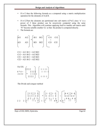
• Let A and B be the 2 n*n Matrix. The product matrix C=AB is calculated by using
the formula,
C (i ,j )= A(i,k) B(k,j) for all ‘i’ and and j between 1 and n.
• The time complexity for the matrix Multiplication is O(n^3).
• Divide and conquer method suggest another way to compute the product of n*n
matrix.
• We assume that N is a power of 2 .In the case N is not a power of 2 ,then enough
rows and columns of zero can be added to both A and B .SO that the resulting
dimension are the powers of two.](https://image.slidesharecdn.com/daanotes-231027021902-07b9e3d5/85/DAA-Notes-pdf-63-320.jpg)


![Design and Analysis of Algorithms
Dept. of CSE, SWEC, Hyderabad Page 65
UNIT-III
GREEDY METHOD:
Greedy Method:
The greedy method is perhaps (maybe or possible) the most straight forward design
technique, used to determine a feasible solution that may or may not be optimal.
Feasible solution:- Most problems have n inputs and its solution contains a subset of
inputs that satisfies a given constraint(condition). Any subset that satisfies the constraint
is called feasible solution.
Optimal solution: To find a feasible solution that either maximizes or minimizes a given
objective function. A feasible solution that does this is called optimal solution.
The greedy method suggests that an algorithm works in stages, considering one input at a
time. At each stage, a decision is made regarding whether a particular input is in an
optimal solution.
Greedy algorithms neither postpone nor revise the decisions (ie., no back tracking).
Example: Kruskal’s minimal spanning tree. Select an edge from a sorted list, check,
decide, and never visit it again.
Application of Greedy Method:
Job sequencing with deadline
0/1 knapsack problem
Minimum cost spanning trees
Single source shortest path problem.
Algorithm for Greedy method
Algorithm Greedy(a,n)
//a[1:n] contains the n inputs.
{
Solution :=0;
For i=1 to n do
{
X:=select(a);
If Feasible(solution, x) then
Solution :=Union(solution,x);
}
Return solution;](https://image.slidesharecdn.com/daanotes-231027021902-07b9e3d5/85/DAA-Notes-pdf-67-320.jpg)
![Design and Analysis of Algorithms
Dept. of CSE, SWEC, Hyderabad Page 66
}
Selection Function, that selects an input from a[] and removes it. The selected input’s
value is assigned to x.
Feasible Boolean-valued function that determines whether x can be included into the
solution vector.
Union function that combines x with solution and updates the objective function.
Knapsack problem
The knapsack problem or rucksack (bag) problem is a problem in combinatorial
optimization: Given a set of items, each with a mass and a value, determine the number
of each item to include in a collection so that the total weight is less than or equal to a
given limit and the total value is as large as possible
There are two versions of the problems
1. 0/1 knapsack problem
2. Fractional Knapsack problem
a. Bounded Knapsack problem.
b. Unbounded Knapsack problem.
Solutions to knapsack problems
Brute-force approach:-Solve the problem with a straight farward algorithm
Greedy Algorithm:- Keep taking most valuable items until maximum weight is
reached or taking the largest value of eac item by calculating vi=valuei/Sizei
Dynamic Programming:- Solve each sub problem once and store their solutions
in an array.
0/1 knapsack problem:](https://image.slidesharecdn.com/daanotes-231027021902-07b9e3d5/85/DAA-Notes-pdf-68-320.jpg)
![Design and Analysis of Algorithms
Dept. of CSE, SWEC, Hyderabad Page 67
Let there be items, to where has a value and weight . The maximum
weight that we can carry in the bag is W. It is common to assume that all values and
weights are nonnegative. To simplify the representation, we also assume that the items
are listed in increasing order of weight.
Maximize subject to
Maximize the sum of the values of the items in the knapsack so that the sum of the weights must
be less than the knapsack's capacity.
Greedy algorithm for knapsack
Algorithm GreedyKnapsack(m,n)
// p[i:n] and [1:n] contain the profits and weights respectively
// if the n-objects ordered such that p[i]/w[i]>=p[i+1]/w[i+1], m size of knapsack
and x[1:n] the solution vector
{
For i:=1 to n do x[i]:=0.0
U:=m;
For i:=1 to n do
{
if(w[i]>U) then break;
x[i]:=1.0;
U:=U-w[i];
}
If(i<=n) then x[i]:=U/w[i];
}
Ex: - Consider 3 objects whose profits and weights are defined as
(P1, P2, P3) = ( 25, 24, 15 )
W1, W2, W3) = ( 18, 15, 10 )
n=3number of objects
m=20Bag capacity
Consider a knapsack of capacity 20. Determine the optimum strategy for placing the
objects in to the knapsack. The problem can be solved by the greedy approach where in
the inputs are arranged according to selection process (greedy strategy) and solve the
problem in stages. The various greedy strategies for the problem could be as follows.
(x1, x2, x3) ∑ xiwi ∑ xipi](https://image.slidesharecdn.com/daanotes-231027021902-07b9e3d5/85/DAA-Notes-pdf-69-320.jpg)


![Design and Analysis of Algorithms
Dept. of CSE, SWEC, Hyderabad Page 70
algorithm js(d, j, n)
//d dead line, jsubset of jobs ,n total number of jobs
// d[i]≥1 1 ≤ i ≤ n are the dead lines,
// the jobs are ordered such that p[1]≥p[2]≥---≥p[n]
//j[i] is the ith job in the optimal solution 1 ≤ i ≤ k, k subset range
{
d[0]=j[0]=0;
j[1]=1;
k=1;
for i=2 to n do{
r=k;
while((d[j[r]]>d[i]) and [d[j[r]]≠r)) do
r=r-1;
if((d[j[r]]≤d[i]) and (d[i]> r)) then
{
for q:=k to (r+1) setp-1 do j[q+1]= j[q];
j[r+1]=i;
k=k+1;
}
}
return k;
}
Note: The size of sub set j must be less than equal to maximum deadline in given list.
Single Source Shortest Paths:
Graphs can be used to represent the highway structure of a state or country with
vertices representing cities and edges representing sections of highway.
The edges have assigned weights which may be either the distance between the 2
cities connected by the edge or the average time to drive along that section of
highway.
For example if A motorist wishing to drive from city A to B then we must answer
the following questions
o Is there a path from A to B
o If there is more than one path from A to B which is the shortest path
The length of a path is defined to be the sum of the weights of the edges on that
path.](https://image.slidesharecdn.com/daanotes-231027021902-07b9e3d5/85/DAA-Notes-pdf-72-320.jpg)

![Design and Analysis of Algorithms
Dept. of CSE, SWEC, Hyderabad Page 72
As an optimization measure we can use the sum of the lengths of all paths so far
generated.
If we have already constructed ‘i’ shortest paths, then using this optimization
measure, the next path to be constructed should be the next shortest minimum
length path.
The greedy way to generate the shortest paths from Vo to the remaining vertices
is to generate these paths in non-decreasing order of path length.
For this 1st
, a shortest path of the nearest vertex is generated. Then a shortest path
to the 2nd
nearest vertex is generated and so on.
Algorithm for finding Shortest Path
Algorithm ShortestPath(v, cost, dist, n)
//dist[j], 1≤j≤n, is set to the length of the shortest path from vertex v to vertex j in graph g
with n-vertices.
// dist[v] is zero
{
for i=1 to n do{
s[i]=false;
dist[i]=cost[v,i];
}
s[v]=true;
dist[v]:=0.0; // put v in s
for num=2 to n do{
// determine n-1 paths from v
choose u form among those vertices not in s such that dist[u] is minimum.
s[u]=true; // put u in s
for (each w adjacent to u with s[w]=false) do
if(dist[w]>(dist[u]+cost[u, w])) then
dist[w]=dist[u]+cost[u, w];
}
}
Minimum Cost Spanning Tree:](https://image.slidesharecdn.com/daanotes-231027021902-07b9e3d5/85/DAA-Notes-pdf-74-320.jpg)


![Design and Analysis of Algorithms
Dept. of CSE, SWEC, Hyderabad Page 81
A dynamic programming formulation for a k-stage graph problem is
obtained by first noticing that every s to t path is the result of a
sequence of k – 2 decisions. The ith decision involves determining
which vertex in vi+1, 1 < i < k - 2, is to be on the path. Let c (i, j) be the
cost of the path from source to destination. Then using the forward
approach, we obtain:
cost (i, j) = min {c (j, l) + cost (i + 1, l)}
l c Vi + 1
<j, l> c E
ALGORITHM:
Algorithm Fgraph (G, k, n, p)
// The input is a k-stage graph G = (V, E) with
n vertices // indexed in order or stages. E is a
set of edges and c [i, j] // is the cost of (i, j). p
[1 : k] is a minimum cost path.
{ co
s
t
[
n
]
:
=
0
.
0
;
for j:= n - 1 to 1 step – 1 do
{ // compute cost [j]
let r be a vertex such that (j, r) is
an edge of G and c [j, r] + cost
[r] is minimum; cost [j] := c](https://image.slidesharecdn.com/daanotes-231027021902-07b9e3d5/85/DAA-Notes-pdf-83-320.jpg)
![Design and Analysis of Algorithms
Dept. of CSE, SWEC, Hyderabad Page 82
[
j
,
r
]
+
c
o
s
t
[
r
]
;
d
[
j
]
:
=
r
:
}
p [1] := 1; p [k] := n; // Find a minimum cost path. for j := 2
to k - 1 do p [j] := d [p [j - 1]];}
The multistage graph problem can also be solved using the backward
approach. Let bp(i, j) be a minimum cost path from vertex s to j vertex in Vi.
Let Bcost(i, j) be the cost of bp(i,
j). From the backward approach we obtain:](https://image.slidesharecdn.com/daanotes-231027021902-07b9e3d5/85/DAA-Notes-pdf-84-320.jpg)
![Design and Analysis of Algorithms
Dept. of CSE, SWEC, Hyderabad Page 83
Bcost (i, j) = min { Bcost (i
–1, l) + c (l,
j)} l e Vi - 1
<l, j> e E
Algorithm Bgraph (G, k, n, p)
// Same function as Fgraph {
Bcost [1] := 0.0; for j := 2 to n do { / / C o m p u t e
B c o s t [ j ] .
Let r be such that (r, j) is an edge of
G and Bcost [r] + c [r, j] is minimum;
Bcost [j] :=
Bcost [r] + c
[r, j]; D [j] :=
r;
} //find a minimum cost path p [1] := 1; p [k] := n;
for j:= k - 1 to 2 do p [j] := d [p [j + 1]];
}
Complexity Analysis:
The complexity analysis of the algorithm is fairly straightforward. Here, if G
has ~E~ edges, then the time for the first for loop is CJ ( V~ +~E ).
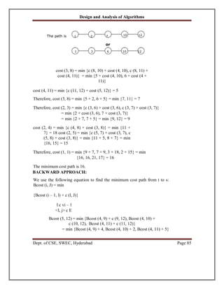
EXAMPLE 1:
Find the minimum cost path from s to t in the multistage graph of five stages
shown below. Do this first using forward approach and then using backward
approach.
FORWARD APPROACH:
We use the following equation to find the minimum cost path
from s to t: cost (i, j) = min {c (j, l) + cost (i + 1, l)}
l c Vi + 1
<j, l> c E](https://image.slidesharecdn.com/daanotes-231027021902-07b9e3d5/85/DAA-Notes-pdf-85-320.jpg)


![Design and Analysis of Algorithms
Dept. of CSE, SWEC, Hyderabad Page 90
k and from k to j must be shortest paths from i to k and k to j,
respectively. Otherwise, the i to j path is not of minimum length. So, the
principle of optimality holds. Let Ak
(i, j) represent the length of a
shortest path from i to j going through no vertex of index greater than k,
we obtain:
Ak (i, j) = {min {min {Ak-1
(i, k) + Ak-1
(k, j)}, c (i, j)} 1<k< n
Algorithm All Paths (Cost, A, n)
// cost [1:n, 1:n] is the cost adjacency matrix
of a graph which // n vertices; A [I, j] is the
cost of a shortest path from vertex // i to
vertex j. cost [i, i] = 0.0, for 1 < i < n.
{ for i := 1 to
n do
for
j:= 1
to n
do
A [i, j] := cost [i, j]; // copy cost into A.
for k := 1 to n
do for
i := 1
to n
do for
j := 1
to n
do
A [i, j] := min (A [i, j], A [i, k] + A [k, j]);
}
Complexity Analysis: A Dynamic programming algorithm based on this
recurrence involves in calculating n+1 matrices, each of size n x n.
Therefore, the algorithm has a complexity of O (n3
).
Example 1:](https://image.slidesharecdn.com/daanotes-231027021902-07b9e3d5/85/DAA-Notes-pdf-92-320.jpg)


![Design and Analysis of Algorithms
Dept. of CSE, SWEC, Hyderabad Page 93
A3 (1, 1) = min {A2
(1, 3) + A2
(3, 1), c (1,
A3 (1, 2) = min {A2
(1, 3) + A2
(3, 2), c (1,
A3 (1, 3) = min {A2
(1, 3) + A2
(3, 3), c (1, A3
(2, 1) = min {A2
(2, 3) + A2
(3, 1), c (2,
A3 (2, 2) = min {A2
(2, 3) + A2
(3, 2), c (2,
A3 (2, 3) = min {A2
(2, 3) + A2
(3, 3), c (2, A3
(3, 1) = min {A2
(3, 3) + A2
(3, 1), c (3,
A3 (3, 2) = min {A2
(3, 3) + A2
(3, 2), c (3,
1)} = min {(6 + 3), 0} = 0
2)} = min {(6 + 7), 4} = 4
3)} = min {(6 + 0), 6} = 6
1)} = min {(2 + 3), 6} = 5
2)} = min {(2 + 7), 0} = 0
3)} = min {(2 + 0), 2} = 2
1)} = min {(0 + 3), 3} = 3
2)} = min {(0 + 7), 7} = 7
107
A3 (3, 3) = min {A2
(3, 3) + A2
(3, 3), c (3, 3)} = min {(0 + 0), 0} = 0
A(3) = ~ 0
~ ~
5~~ 3
4
0
7
6 ~
~
2~
0
~]
TRAVELLING SALESPERSON PROBLEM
Let G = (V, E) be a directed graph with edge costs Cij. The variable cij is defined such
that cij > 0 for all I and j and cij = a if < i, j> o E. Let |V| = n and assume n > 1. A tour
of G is a directed simple cycle that includes every vertex in V. The cost of a tour is the
sum of the cost of the edges on the tour. The traveling sales person problem is to find a
tour of minimum cost. The tour is to be a simple path that starts and ends at vertex 1.
Let g (i, S) be the length of shortest path starting at vertex i, going through all vertices
in S, and terminating at vertex 1. The function g (1, V – {1}) is the length of an optimal
salesperson tour. From the principal of optimality it follows that:
g(1, V - {1 }) = 2 ~ k ~ n ~c1k ~ g ~ k, V ~ ~ 1, k ~~ -- 1
~
min
-- 2
Generalizing equation 1, we obtain (for i o S)
g ( i, S ) = min{ci j j ES
The Equation can be solved for g (1, V – 1}) if we know g (k, V – {1, k})
for all choices of k.](https://image.slidesharecdn.com/daanotes-231027021902-07b9e3d5/85/DAA-Notes-pdf-95-320.jpg)
![Design and Analysis of Algorithms
Dept. of CSE, SWEC, Hyderabad Page 94
Complexity Analysis:
For each value of |S| there + g (
i, S
-{
j } ) } are n – 1 choices for i. The number of distinct
sets S of
size k not including 1 and i is I k ~
~
~ .
n - 2
~
~
~ ~
Hence, the total number of g (i, S)’s to be computed before computing g (1, V – {1}) is:
~ n - 2 ~
~ ~n ~1~ ~
~ k ~
k ~ 0 ~ ~
To calculate this sum, we use the binominal theorem:
[((n - 2) ((n - 2) ((n - 2) ((n - 2)1 n - 1 (n – 1) 111 11+ ii iI+
ii iI+ - - - - ~ ~~
~~ 0 ) ~ 1 ) ~ 2 ) ~(n ~ 2
)~~
According to the binominal theorem:
[((n - 2) ((n - 2) ((n - 2 ((n - 2)1
il 11+ ii iI+ ii ~~~ ~ ~ ~ ~ ~ ~~ ~~~ = 2n - 2
~~ 0 ~ ~ 1 ~ ~ 2 ~ ~(n - 2))]
Therefore,
n - 1 ~ n _ 2'
~ ( n _ 1~ ~~ ~k = (n - 1) 2n ~ 2
k ~ 0 ~ ~
This is Φ (n 2n-2
), so there are exponential number of calculate. Calculating one g (i, S)
require finding the minimum of at most n quantities. Therefore, the entire algorithm is
Φ (n2
2n-2
). This is better than enumerating all n! different tours to find the best one. So,
we have traded on exponential growth for a much smaller exponential growth.
The most serious drawback of this dynamic programming solution is the space needed,
which is O (n 2n
). This is too large even for modest values of n.
Example 1:](https://image.slidesharecdn.com/daanotes-231027021902-07b9e3d5/85/DAA-Notes-pdf-96-320.jpg)
![Design and Analysis of Algorithms
Dept. of CSE, SWEC, Hyderabad Page 95
For the following graph find minimum cost tour for the traveling
salesperson problem:
r0 10 15 2
~ 10
~
The cost adjacency matrix = ~
0 9 12~
5 13 0 ~ ~6 8 9 0 1]
~
Let us start the tour from vertex 1:
g (1, V – {1}) = min {c1k + g (k, V – {1, K})}
2<k<n
More generally writing:
- (1)
g (i, s) = min {cij + g (J, s – {J})} - (2)
Clearly, g (i, T) = ci1 , 1 ≤ i ≤ n. So,
g (2, T) = C21
= 5 g (3, T) = C31 = 6
g (4, ~) = C41 = 8
Using equation – (2)
we obtain:
g (1, {2, 3, 4}) = min {c12 + g (2, {3,
4}, c13 + g (3, {2, 4}), c14 + g (4, {2, 3})}
g (2, {3, 4}) = min {c23 + g (3, {4}), c24 + g (4, {3})}
= min {9 + g (3, {4}), 10 + g (4, {3})} g (3,
{4}) = min {c34 + g (4, T)} = 12 + 8 = 20 g
(4, {3}) = min {c43 + g (3, ~)} = 9 + 6 = 15
Therefore, g (2, {3, 4}) = min {9 + 20, 10 +
1 2
3 4](https://image.slidesharecdn.com/daanotes-231027021902-07b9e3d5/85/DAA-Notes-pdf-97-320.jpg)


![Design and Analysis of Algorithms
Dept. of CSE, SWEC, Hyderabad Page 101
0 2, 0, 0 3, 0, 0 1, 0, 0 1, 0, 0, 1, 0, 0
1 8, 8, 1 7, 7, 2 3, 3, 3 3, 3, 4
2 12, 19, 1 9, 12, 2 5, 8, 3
3 14, 25, 2 11, 19, 2
4 16, 32, 2
This computation is carried out row-wise from row 0 to row 4. Initially, W (i, i) = Q (i)
and C (i, i) = 0 and R (i, i) = 0, 0 < i < 4.
Solving for C (0, n):
First, computing all C (i, j) such that j - i = 1; j = i + 1 and as 0 < i < 4; i = 0, 1, 2 and
3; i < k ≤ J. Start with i = 0; so j = 1; as i < k ≤ j, so the possible value for k = 1
W (0, 1) = P (1) + Q (1) + W (0, 0) = 3 + 3 + 2 = 8
C (0, 1) = W (0, 1) + min {C (0, 0) + C (1, 1)} = 8
R (0, 1) = 1 (value of 'K' that is minimum in the above equation).
Next with i = 1; so j = 2; as i < k ≤ j, so the possible value for k = 2
W (1, 2) = P (2) + Q (2) + W (1, 1) = 3 + 1 + 3 = 7
C (1, 2) = W (1, 2) + min {C (1, 1) + C (2, 2)} = 7
R (1, 2) = 2
Next with i = 2; so j = 3; as i < k ≤ j, so the possible value for k = 3
W (2, 3) = P (3) + Q (3) + W (2, 2) = 1 + 1 + 1 = 3
C (2, 3) = W (2, 3) + min {C (2, 2) + C (3, 3)} = 3 + [(0 + 0)] = 3 ft
(2, 3) = 3
Next with i = 3; so j = 4; as i < k ≤ j, so the possible value for k = 4
W (3, 4) = P (4) + Q (4) + W (3, 3) = 1 + 1 + 1 = 3
C (3, 4) = W (3, 4) + min {[C (3, 3) + C (4, 4)]} = 3 + [(0 + 0)] = 3 ft
(3, 4) = 4
Second, Computing all C (i, j) such that j - i = 2; j = i + 2 and as 0 < i < 3; i = 0, 1, 2; i
< k ≤ J. Start with i = 0; so j = 2; as i < k ≤ J, so the possible values for k = 1 and 2.
W (0, 2) = P (2) + Q (2) + W (0, 1) = 3 + 1 + 8 = 12](https://image.slidesharecdn.com/daanotes-231027021902-07b9e3d5/85/DAA-Notes-pdf-103-320.jpg)
![Design and Analysis of Algorithms
Dept. of CSE, SWEC, Hyderabad Page 102
C (0, 2) = W (0, 2) + min {(C (0, 0) + C (1, 2)), (C (0, 1) + C (2, 2))} = 12
+ min {(0 + 7, 8 + 0)} = 19
ft (0, 2) = 1
Next, with i = 1; so j = 3; as i < k ≤ j, so the possible value for k = 2 and 3.
W (1, 3) = P (3) + Q (3) + W (1, 2) = 1 + 1+ 7 = 9
C (1, 3) = W (1, 3) + min {[C (1, 1) + C (2, 3)], [C (1, 3) 2) + C (3, 3)]}
= W (1, + min {(0 + 3), (7 + 0)} = 9 + 3 = 12
ft (1, 3) = 2
Next, with i = 2; so j = 4; as i < k ≤ j, so the possible value for k = 3 and 4.
W (2, 4) = P (4) + Q (4) + W (2, 3) = 1 + 1 + 3 = 5
C (2, 4) = W (2, 4) + min {[C (2, 2) + C (3, 4)], [C (2, 3) + C (4, 4)]
= 5 + min {(0 + 3), (3 + 0)} = 5 + 3 = 8
ft (2, 4) = 3
Third, Computing all C (i, j) such that J - i = 3; j = i + 3 and as 0 < i < 2; i = 0, 1; i < k
≤ J. Start with i = 0; so j = 3; as i < k ≤ j, so the possible values for k = 1, 2 and 3.
W (0, 3) = P (3) + Q (3) + W (0, 2) = 1 + 1 =
+ 12 = 14
C (0, 3) W (0, 3) + min {[C (0, 0) + C (1,
3)], [C (0,
1) + C (2,
3)],
[C (0, 2) + C (3, =
3)]}
14 + min {(0 + 12), (8 + 3), (19 = 2 + 0)} = 14 + 11 = 25
ft (0, 3)
Start with i = 1; so j = 4; as i < k ≤ j, so the possible values for k = 2, 3 and
4.
W (1, 4) = P (4) + Q (4) + W (1, 3) = 1 + 1 + 9 = 11 = W 2)
C (1, 4) (1, 4) + min {[C (1, 1) + C (2, 4)], [C (1, + C (3, 4)],
= 11 + min {(0 + 8), (7 + 3), (12 + 0)} = 11 [C (1, 3) + C (4, 4)]} = 2 + 8 = 19
ft (1, 4)
Fourth, Computing all C (i, j) such that j - i = 4; j = i + 4 and as 0 < i < 1; i = 0; i < k ≤
J.
Start with i = 0; so j = 4; as i < k ≤ j, so the possible values for k = 1, 2, 3 and 4.](https://image.slidesharecdn.com/daanotes-231027021902-07b9e3d5/85/DAA-Notes-pdf-104-320.jpg)
![Design and Analysis of Algorithms
Dept. of CSE, SWEC, Hyderabad Page 103
W (0, 4) = P (4) + Q (4) + W (0, 3) = 1 + 1 + 14 = 16
C (0, 4) = W (0, 4) + min {[C (0, 0) + C (1, 4)], [C (0, 1) + C (2, 4)],
[C (0, 2) + C (3, 4)], [C (0, 3) + C (4, 4)]}
= 16 + min [0 + 19, 8 + 8, 19+3, 25+0] = 16 + 16 = 32 ft (0,
4) = 2
From the table we see that C (0, 4) = 32 is the minimum cost of a binary search tree for
(a1, a2, a3, a4). The root of the tree 'T04' is 'a2'.
Hence the left sub tree is 'T01' and right sub tree is T24. The root of 'T01' is 'a1' and the
root of 'T24' is a3.
The left and right sub trees for 'T01' are 'T00' and 'T11' respectively. The root of T01 is
'a1'
The left and right sub trees for T24 are T22 and T34 respectively.
The root of T24 is 'a3'.
The root of T22 is null
The root of T34 is a4.
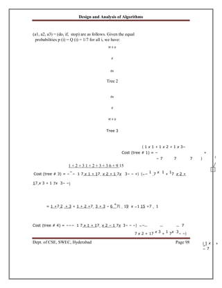
Example 2:
Consider four elements a1, a2, a3 and a4 with Q0 = 1/8, Q1 = 3/16, Q2 = Q3 = Q4 =
1/16 and p1 = 1/4, p2 = 1/8, p3 = p4 =1/16. Construct an optimal binary search tree.
Solving for C (0, n):
First, computing all C (i, j) such that j - i = 1; j = i + 1 and as 0 < i < 4; i = 0, 1, 2 and
3; i
< k ≤ J. Start with i = 0; so j = 1; as i < k ≤ j, so the possible value for k = 1
W (0, 1) = P (1) + Q (1) + W (0, 0) = 4 + 3 + 2 = 9
a2
T 04
a1 a3
T 01 T 24
T 00 T 11 T 22 T 34
a4
do read
if
while](https://image.slidesharecdn.com/daanotes-231027021902-07b9e3d5/85/DAA-Notes-pdf-105-320.jpg)
![Design and Analysis of Algorithms
Dept. of CSE, SWEC, Hyderabad Page 104
C (0, 1) = W (0, 1) + min {C (0, 0) + C (1, 1)} = 9 + [(0 + 0)] = 9 ft
(0, 1) = 1 (value of 'K' that is minimum in the above equation).
Next with i = 1; so j = 2; as i < k ≤ j, so the possible value for k = 2
W (1, 2) = P (2) + Q (2) + W (1, 1) = 2 + 1 + 3 = 6
C (1, 2) = W (1, 2) + min {C (1, 1) + C (2, 2)} = 6 + [(0 + 0)] = 6 ft
(1, 2) = 2
Next with i = 2; so j = 3; as i < k ≤ j, so the possible value for k = 3
+ 1 = 3
W (2, 3) = P (3) + Q (3) + W (2, 2) = 1 + 1 3)} = 3 + [(0 + 0)] = 3 C (2,
3) = W (2, 3) + min {C (2, 2) + C (3, ft (2, 3) = 3
Next with i = 3; so j = 4; as i < k ≤ j, so the possible value for k = 4
W (3, 4) = P (4) + Q (4) + W (3, 3) = 1 + 1 + 1 = 3
C (3, 4) = W (3, 4) + min {[C (3, 3) + C (4, 4)]} = 3 + [(0 + 0)] = 3 ft
(3, 4) = 4
Second, Computing all C (i, j) such that j - i = 2; j = i + 2 and as 0 < i < 3; i = 0, 1, 2;
i < k ≤ J
Start with i = 0; so j = 2; as i < k ≤ j, so the possible values for k = 1 and 2.
W (0, 2) = P (2) + Q (2) + W (0, 1) = 2 + 1 + 9 = 12
C (0, 2) = W (0, 2) + min {(C (0, 0) + C (1, 2)), (C (0, 1) + C (2, 2))} =
12 + min {(0 + 6, 9 + 0)} = 12 + 6 = 18 ft (0, 2) = 1
Next, with i = 1; so j = 3; as i < k ≤ j, so the possible value for k = 2 and 3.
W (1, 3) = P (3) + Q (3) + W (1, 2) = 1 + 1+ 6 = 8
C (1, 3) = W (1, 3) + min {[C (1, 1) + C (2, 3)], [C (1, 2) + C (3, 3)]}
= W (1, 3) + min {(0 + 3), (6 + 0)} = 8 + 3 = 11
ft (1, 3) = 2
Next, with i = 2; so j = 4; as i < k ≤ j, so the possible value for k = 3 and 4.
W (2, 4) = P (4) + Q (4) + W (2, 3) = 1 + 1 + 3 = 5
C (2, 4) = W (2, 4) + min {[C (2, 2) + C (3, 4)], [C (2, 3) + C (4, 4)]
= 5 + min {(0 + 3), (3 + 0)} = 5 + 3 = 8
ft (2, 4) = 3](https://image.slidesharecdn.com/daanotes-231027021902-07b9e3d5/85/DAA-Notes-pdf-106-320.jpg)
![Design and Analysis of Algorithms
Dept. of CSE, SWEC, Hyderabad Page 105
Third, Computing all C (i, j) such that J - i = 3; j = i + 3 and as 0 < i < 2; i = 0, 1; i < k
≤ J. Start with i = 0; so j = 3; as i < k ≤ j, so the possible values for k = 1, 2 and 3.
W (0, 3) = P (3) + Q (3) + W (0, 2) = 1 + 1 + 12 = 14
C (0, 3) = W (0, 3) + min {[C (0, 0) + C (1, 3)], [C (0, 1) + C (2, 3)], [C (0,
2) + C (3, 3)]}
= 14 + min {(0 + 11), (9 + 3), (18 + 0)} = 14 + 11 = 25 ft (0,
3) = 1
Start with i = 1; so j = 4; as i < k ≤ j, so the possible values for k = 2, 3 and
4.
W (1, 4) = P (4) + Q (4) + W (1, 3) = 1 + 1 + 8 = 10 = W 2)
C (1, 4) (1, 4) + min {[C (1, 1) + C (2, 4)], [C (1, + C (3, 4)],
= 10 + min {(0 + 8), (6 + 3), (11 + 0)} = 10 [C (1, 3) + C (4, 4)]} = 2 + 8 = 18
ft (1, 4)
Fourth, Computing all C (i, j) such that J - i = 4; j = i + 4 and as 0 < i < 1; i = 0; i <
k ≤ J. Start with i = 0; so j = 4; as i < k ≤ j, so the possible values for k = 1, 2, 3 and
4.
W (0, 4) = P (4) + Q (4) + W (0, 3) = 1 + 1 + 14 = 16
C (0, 4) = W (0, 4) + min {[C (0, 0) + C (1, 4)], [C (0, 1) + C (2, 4)],
[C (0, 2) + C (3, 4)], [C (0, 3) + C (4, 4)]}
= 16 + min [0 + 18, 9 + 8, 18 + 3, 25 + 0] = 16 + 17 = 33 R (0, 4)
= 2
Table for recording W (i, j), C (i, j) and R (i, j)
Column
Row
0 1 2 3 4
0 2, 0, 0 1, 0, 0 1, 0, 0 1, 0, 0, 1, 0, 0
1 9, 9, 1 6, 6, 2 3, 3, 3 3, 3, 4
2 12, 18, 1 8, 11, 2 5, 8, 3
3 14, 25, 2 11, 18, 2](https://image.slidesharecdn.com/daanotes-231027021902-07b9e3d5/85/DAA-Notes-pdf-107-320.jpg)


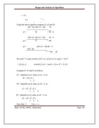


![Design and Analysis of Algorithms
Dept. of CSE, SWEC, Hyderabad Page 118
One or more sequences of choices may or may not lead to a solution.
Many types of maze problem can be solved with backtracking.
Example@ 2 (text book):
Sorting the array of integers in a[1:n] is a problem whose solution is expressible by an n-
tuple
xi is the index in ‘a’ of the ith
smallest element.
The criterion function ‘P’ is the inequality a[xi]≤ a[xi+1] for 1≤ i ≤ n
Si is finite and includes the integers 1 through n.
misize of set Si
m=m1m2m3---mn n tuples that possible candidates for satisfying the function P.
With brute force approach would be to form all these n-tuples, evaluate (judge) each one
with P and save those which yield the optimum.
By using backtrack algorithm; yield the same answer with far fewer than ‘m’ trails.
Many of the problems we solve using backtracking requires that all the solutions satisfy a
complex set of constraints.
For any problem these constraints can be divided into two categories:
Explicit constraints.
Implicit constraints.
Explicit constraints: Explicit constraints are rules that restrict each xi to take on values
only from a given set.
Example: xi ≥ 0 or si={all non negative real numbers}
Xi=0 or 1 or Si={0, 1}
li ≤ xi ≤ ui or si={a: li ≤ a ≤ ui }
The explicit constraint depends on the particular instance I of the problem being solved.
All tuples that satisfy the explicit constraints define a possible solution space for I.](https://image.slidesharecdn.com/daanotes-231027021902-07b9e3d5/85/DAA-Notes-pdf-120-320.jpg)


![Design and Analysis of Algorithms
Dept. of CSE, SWEC, Hyderabad Page 122
if(x[j]=i or Abs(x[j]-i)=Abs(j-k)))
then return false
return true
}
{
X[k]:=I;
if(k==n) then write (x[1:n]);
else NQueens(k+1, n);
}
}}
Sum of Subsets Problem:](https://image.slidesharecdn.com/daanotes-231027021902-07b9e3d5/85/DAA-Notes-pdf-124-320.jpg)

![Design and Analysis of Algorithms
Dept. of CSE, SWEC, Hyderabad Page 124
The equation cannot lead to solution.
Recursive backtracking algorithm for sum of subsets problem
Algorithm SumOfSub(s, k, r)
{
X[k]=1
If(S+w[k]=m) then write(x[1: ]); // subset found.
Else if (S+w[k] + w{k+1] ≤ M)
Then SumOfSub(S+w[k], k+1, r-w[k]);
if ((S+r - w{k] ≥ M) and (S+w[k+1] ≤M) ) then
{
X[k]=0;
SumOfSub(S, k+1, r-w[k]);
}
}](https://image.slidesharecdn.com/daanotes-231027021902-07b9e3d5/85/DAA-Notes-pdf-126-320.jpg)

![Design and Analysis of Algorithms
Dept. of CSE, SWEC, Hyderabad Page 126
A graph is said to be planar iff it can be drawn in a plane (flat) in such a way that
no two edges cross each other.
M-Colorability decision problem is the 4-color problem for planar graphs.
Given any map, can the regions be colored in such a way that no two adjacent
regions have the same color yet only 4-colors are needed?
To solve this problem, graphs are very useful, because a map can easily be
transformed into a graph.
Each region of the map becomes a node, and if two regions are adjacent, then the
corresponding nodes are joined by an edge.
o Example:
o
The above map requires 4 colors.
Many years, it was known that 5-colors were required to color this map.
After several hundred years, this problem was solved by a group of
mathematicians with the help of a computer. They show that 4-colors are
sufficient.
Suppose we represent a graph by its adjacency matrix G[1:n, 1:n]
Ex:](https://image.slidesharecdn.com/daanotes-231027021902-07b9e3d5/85/DAA-Notes-pdf-128-320.jpg)
![Design and Analysis of Algorithms
Dept. of CSE, SWEC, Hyderabad Page 127
Here G[i, j]=1 if (i, j) is an edge of G, and G[i, j]=0 otherwise.
Colors are represented by the integers 1, 2,---m and the solutions are given by the n-tuple
(x1, x2,---xn)
xi Color of node i.
State Space Tree for
n=3 nodes
m=3colors
1st
node coloured in 3-ways
2nd
node coloured in 3-ways
3rd
node coloured in 3-ways
So we can colour in the graph in 27 possibilities of colouring.](https://image.slidesharecdn.com/daanotes-231027021902-07b9e3d5/85/DAA-Notes-pdf-129-320.jpg)
![Design and Analysis of Algorithms
Dept. of CSE, SWEC, Hyderabad Page 128
Finding all m-coloring of a graph Getting next color
Algorithm mColoring(k){
// g(1:n, 1:n) boolean adjacency matrix.
// kindex (node) of the next vertex to
color.
repeat{
nextvalue(k); // assign to x[k] a legal
color.
if(x[k]=0) then return; // no new color
possible
if(k=n) then write(x[1: n];
else mcoloring(k+1);
}
until(false)
}
Algorithm NextValue(k){
//x[1],x[2],---x[k-1] have been assigned
integer values in the range [1, m]
repeat {
x[k]=(x[k]+1)mod (m+1); //next highest
color
if(x[k]=0) then return; // all colors have
been used.
for j=1 to n do
{
if ((g[k,j]≠0) and (x[k]=x[j]))
then break;
}
if(j=n+1) then return; //new color found
} until(false)
}
Previous paper example:
Adjacency matrix is](https://image.slidesharecdn.com/daanotes-231027021902-07b9e3d5/85/DAA-Notes-pdf-130-320.jpg)

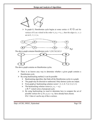
![Design and Analysis of Algorithms
Dept. of CSE, SWEC, Hyderabad Page 131
By using “NextValue” algorithm the recursive backtracking scheme to find all
Hamiltoman cycles.
This algorithm is started by 1st
initializing the adjacency matrix G[1:n, 1:n] then setting
x[2:n] to zero & x[1] to 1, and then executing Hamiltonian (2)
Generating Next Vertex Finding all Hamiltonian Cycles
Algorithm NextValue(k)
{
// x[1: k-1] is path of k-1 distinct
vertices.
// if x[k]=0, then no vertex has yet been
assigned to x[k]
Repeat{
X[k]=(x[k]+1) mod (n+1); //Next vertex
If(x[k]=0) then return;
If(G[x[k-1], x[k]]≠0) then
{
For j:=1 to k-1 do if(x[j]=x[k]) then
break;
//Check for distinctness
If(j=k) then //if true , then vertex is
distinct
If((k<n) or (k=n) and G[x[n], x[1]]≠0))
Then return ;
}
}
Until (false);
}
Algorithm Hamiltonian(k)
{
Repeat{
NextValue(k); //assign a legal next value to
x[k]
If(x[k]=0) then return;
If(k=n) then write(x[1:n]);
Else Hamiltonian(k+1);
} until(false)
}](https://image.slidesharecdn.com/daanotes-231027021902-07b9e3d5/85/DAA-Notes-pdf-133-320.jpg)


![Design and Analysis of Algorithms
Dept. of CSE, SWEC, Hyderabad Page 137
A row (column) is said to be reduced iff it contains at least one zero & remaining entries are
non negative.
A matrix is reduced iff every row & column is reduced.
Given the following cost matrix:
[
𝑖𝑛𝑓 20 30 10 11
15 𝑖𝑛𝑓 16 4 2
3 5 𝑖𝑛𝑓 2 4
19 6 18 𝑖𝑛𝑓 3
16 4 7 16 𝑖𝑛𝑓 ]
The TSP starts from node 1: Node 1
Reduced Matrix: To get the lower bound of the path starting at node 1
Row # 1: reduce by 10
[
𝑖𝑛𝑓 10 20 0 1
15 𝑖𝑛𝑓 16 4 2
3 5 𝑖𝑛𝑓 2 4
19 6 18 𝑖𝑛𝑓 3
16 4 7 16 𝑖𝑛𝑓 ]
Row #2: reduce 2
[
𝑖𝑛𝑓 10 20 0 1
13 𝑖𝑛𝑓 14 2 0
3 5 𝑖𝑛𝑓 2 4
19 6 18 𝑖𝑛𝑓 3
16 4 7 16 𝑖𝑛𝑓 ]
Row #3: reduce by 2
[
𝑖𝑛𝑓 10 20 0 1
13 𝑖𝑛𝑓 14 2 0
1 3 𝑖𝑛𝑓 0 2
19 6 18 𝑖𝑛𝑓 3
16 4 7 16 𝑖𝑛𝑓 ]
Row # 4: Reduce by 3:
[
𝑖𝑛𝑓 10 20 0 1
13 𝑖𝑛𝑓 14 2 0
1 3 𝑖𝑛𝑓 0 2
16 3 15 𝑖𝑛𝑓 0
16 4 7 16 𝑖𝑛𝑓 ]
Row # 5: Reduce by 4
[
𝑖𝑛𝑓 10 20 0 1
13 𝑖𝑛𝑓 14 2 0
1 3 𝑖𝑛𝑓 0 2
16 3 15 𝑖𝑛𝑓 0
12 0 3 12 𝑖𝑛𝑓 ]
Column 1: Reduce by 1
[
𝑖𝑛𝑓 10 20 0 1
12 𝑖𝑛𝑓 14 2 0
0 3 𝑖𝑛𝑓 0 2
15 3 15 𝑖𝑛𝑓 0
11 0 3 12 𝑖𝑛𝑓 ]](https://image.slidesharecdn.com/daanotes-231027021902-07b9e3d5/85/DAA-Notes-pdf-139-320.jpg)
![Design and Analysis of Algorithms
Dept. of CSE, SWEC, Hyderabad Page 138
Column 2: It is reduced. Column 3: Reduce by 3 Column 4: It is reduced.
Column 5: It is reduced.
The reduced cost is: RCL = 25
So the cost of node 1 is: Cost (1) = 25
The reduced matrix is:
Choose to go to vertex 2: Node 2
- Cost of edge <1,2> is: A(1,2) = 10
- Set row #1 = inf since we are choosing edge <1,2>
- Set column # 2 = inf since we are choosing edge <1,2>
- Set A(2,1) = inf
- The resulting cost matrix is:
[
𝑖𝑛𝑓 𝑖𝑛𝑓 𝑖𝑛𝑓 𝑖𝑛𝑓 𝑖𝑛𝑓
𝑖𝑛𝑓 𝑖𝑛𝑓 11 2 0
0 𝑖𝑛𝑓 𝑖𝑛𝑓 0 2
15 𝑖𝑛𝑓 12 𝑖𝑛𝑓 0
11 𝑖𝑛𝑓 0 12 𝑖𝑛𝑓 ]
- The matrix is reduced:
- RCL = 0
- The cost of node 2 (Considering vertex 2 from vertex 1) is:
Cost(2) = cost(1) + A(1,2) = 25 + 10 = 35
Choose to go to vertex 3: Node 3
- Cost of edge <1,3> is: A(1,3) = 17 (In the reduced matrix
- Set row #1 = inf since we are starting from node 1
- Set column # 3 = inf since we are choosing edge <1,3>
- Set A(3,1) = inf
- The resulting cost matrix is:](https://image.slidesharecdn.com/daanotes-231027021902-07b9e3d5/85/DAA-Notes-pdf-140-320.jpg)
![Design and Analysis of Algorithms
Dept. of CSE, SWEC, Hyderabad Page 139
[
𝑖𝑛𝑓 𝑖𝑛𝑓 𝑖𝑛𝑓 𝑖𝑛𝑓 𝑖𝑛𝑓
12 𝑖𝑛𝑓 𝑖𝑛𝑓 2 0
𝑖𝑛𝑓 3 𝑖𝑛𝑓 0 2
15 3 𝑖𝑛𝑓 𝑖𝑛𝑓 0
11 0 𝑖𝑛𝑓 12 𝑖𝑛𝑓 ]
Reduce the matrix: Rows are reduced
The columns are reduced except for column # 1:
Reduce column 1 by 11:
[
𝑖𝑛𝑓 𝑖𝑛𝑓 𝑖𝑛𝑓 𝑖𝑛𝑓 𝑖𝑛𝑓
1 𝑖𝑛𝑓 𝑖𝑛𝑓 2 0
𝑖𝑛𝑓 3 𝑖𝑛𝑓 0 2
4 3 𝑖𝑛𝑓 𝑖𝑛𝑓 0
0 0 𝑖𝑛𝑓 12 𝑖𝑛𝑓 ]
The lower bound is: RCL = 11
The cost of going through node 3 is:
cost(3) = cost(1) + RCL + A(1,3) = 25 + 11 + 17 = 53
Choose to go to vertex 4: Node 4
Remember that the cost matrix is the one that was reduced at the starting vertex 1
Cost of edge <1,4> is: A(1,4) = 0
Set row #1 = inf since we are starting from node 1
Set column # 4 = inf since we are choosing edge <1,4>
Set A(4,1) = inf
The resulting cost matrix is:
[
𝑖𝑛𝑓 𝑖𝑛𝑓 𝑖𝑛𝑓 𝑖𝑛𝑓 𝑖𝑛𝑓
12 𝑖𝑛𝑓 11 𝑖𝑛𝑓 0
0 3 𝑖𝑛𝑓 𝑖𝑛𝑓 2
𝑖𝑛𝑓 3 12 𝑖𝑛𝑓 0
11 0 0 𝑖𝑛𝑓 𝑖𝑛𝑓 ]
Reduce the matrix: Rows are reduced
Columns are reduced
The lower bound is: RCL = 0
The cost of going through node 4 is:
cost(4) = cost(1) + RCL + A(1,4) = 25 + 0 + 0 = 25](https://image.slidesharecdn.com/daanotes-231027021902-07b9e3d5/85/DAA-Notes-pdf-141-320.jpg)
![Design and Analysis of Algorithms
Dept. of CSE, SWEC, Hyderabad Page 140
Choose to go to vertex 5: Node 5
- Remember that the cost matrix is the one that was reduced at starting vertex 1
- Cost of edge <1,5> is: A(1,5) = 1
- Set row #1 = inf since we are starting from node 1
- Set column # 5 = inf since we are choosing edge <1,5>
- Set A(5,1) = inf
- The resulting cost matrix is:
[
𝑖𝑛𝑓 𝑖𝑛𝑓 𝑖𝑛𝑓 𝑖𝑛𝑓 𝑖𝑛𝑓
12 𝑖𝑛𝑓 11 2 𝑖𝑛𝑓
0 3 𝑖𝑛𝑓 0 𝑖𝑛𝑓
15 3 12 𝑖𝑛𝑓 𝑖𝑛𝑓
𝑖𝑛𝑓 0 0 12 𝑖𝑛𝑓 ]
Reduce the matrix:
Reduce rows:
Reduce row #2: Reduce by 2
[
𝑖𝑛𝑓 𝑖𝑛𝑓 𝑖𝑛𝑓 𝑖𝑛𝑓 𝑖𝑛𝑓
10 𝑖𝑛𝑓 9 0 𝑖𝑛𝑓
0 3 𝑖𝑛𝑓 0 𝑖𝑛𝑓
15 3 12 𝑖𝑛𝑓 𝑖𝑛𝑓
𝑖𝑛𝑓 0 0 12 𝑖𝑛𝑓 ]
Reduce row #4: Reduce by 3
[
𝑖𝑛𝑓 𝑖𝑛𝑓 𝑖𝑛𝑓 𝑖𝑛𝑓 𝑖𝑛𝑓
10 𝑖𝑛𝑓 9 0 𝑖𝑛𝑓
0 3 𝑖𝑛𝑓 0 𝑖𝑛𝑓
12 0 9 𝑖𝑛𝑓 𝑖𝑛𝑓
𝑖𝑛𝑓 0 0 12 𝑖𝑛𝑓 ]
Columns are reduced
The lower bound is: RCL = 2 + 3 = 5
The cost of going through node 5 is:
cost(5) = cost(1) + RCL + A(1,5) = 25 + 5 + 1 = 31](https://image.slidesharecdn.com/daanotes-231027021902-07b9e3d5/85/DAA-Notes-pdf-142-320.jpg)
![Design and Analysis of Algorithms
Dept. of CSE, SWEC, Hyderabad Page 141
In summary:
So the live nodes we have so far are:
2: cost(2) = 35, path: 1->2
3: cost(3) = 53, path: 1->3
4: cost(4) = 25, path: 1->4
5: cost(5) = 31, path: 1->5
Explore the node with the lowest cost: Node 4 has a cost of 25
Vertices to be explored from node 4: 2, 3, and 5
Now we are starting from the cost matrix at node 4 is:
Choose to go to vertex 2: Node 6 (path is 1->4->2)
Cost of edge <4,2> is: A(4,2) = 3
Set row #4 = inf since we are considering edge <4,2>
Set column # 2 = inf since we are considering edge <4,2>
Set A(2,1) = inf
The resulting cost matrix is:
[
𝑖𝑛𝑓 𝑖𝑛𝑓 𝑖𝑛𝑓 𝑖𝑛𝑓 𝑖𝑛𝑓
𝑖𝑛𝑓 𝑖𝑛𝑓 11 𝑖𝑛𝑓 0
0 𝑖𝑛𝑓 𝑖𝑛𝑓 𝑖𝑛𝑓 2
𝑖𝑛𝑓 𝑖𝑛𝑓 𝑖𝑛𝑓 𝑖𝑛𝑓 𝑖𝑛𝑓
11 𝑖𝑛𝑓 0 𝑖𝑛𝑓 𝑖𝑛𝑓 ]
Reduce the matrix: Rows are reduced
Columns are reduced
The lower bound is: RCL = 0
The cost of going through node 2 is:
cost(6) = cost(4) + RCL + A(4,2) = 25 + 0 + 3 = 28](https://image.slidesharecdn.com/daanotes-231027021902-07b9e3d5/85/DAA-Notes-pdf-143-320.jpg)
![Design and Analysis of Algorithms
Dept. of CSE, SWEC, Hyderabad Page 142
Choose to go to vertex 3: Node 7 ( path is 1->4->3 )
Cost of edge <4,3> is: A(4,3) = 12
Set row #4 = inf since we are considering edge <4,3>
Set column # 3 = inf since we are considering edge <4,3>
Set A(3,1) = inf
The resulting cost matrix is:
[
𝑖𝑛𝑓 𝑖𝑛𝑓 𝑖𝑛𝑓 𝑖𝑛𝑓 𝑖𝑛𝑓
12 𝑖𝑛𝑓 𝑖𝑛𝑓 𝑖𝑛𝑓 0
𝑖𝑛𝑓 3 𝑖𝑛𝑓 𝑖𝑛𝑓 2
𝑖𝑛𝑓 𝑖𝑛𝑓 𝑖𝑛𝑓 𝑖𝑛𝑓 𝑖𝑛𝑓
11 0 𝑖𝑛𝑓 𝑖𝑛𝑓 𝑖𝑛𝑓 ]
Reduce the matrix:
Reduce row #3: by 2:
[
𝑖𝑛𝑓 𝑖𝑛𝑓 𝑖𝑛𝑓 𝑖𝑛𝑓 𝑖𝑛𝑓
12 𝑖𝑛𝑓 𝑖𝑛𝑓 𝑖𝑛𝑓 0
𝑖𝑛𝑓 1 𝑖𝑛𝑓 𝑖𝑛𝑓 0
𝑖𝑛𝑓 𝑖𝑛𝑓 𝑖𝑛𝑓 𝑖𝑛𝑓 𝑖𝑛𝑓
11 0 𝑖𝑛𝑓 𝑖𝑛𝑓 𝑖𝑛𝑓 ]
Reduce column # 1: by 11
[
𝑖𝑛𝑓 𝑖𝑛𝑓 𝑖𝑛𝑓 𝑖𝑛𝑓 𝑖𝑛𝑓
1 𝑖𝑛𝑓 𝑖𝑛𝑓 𝑖𝑛𝑓 0
𝑖𝑛𝑓 1 𝑖𝑛𝑓 𝑖𝑛𝑓 0
𝑖𝑛𝑓 𝑖𝑛𝑓 𝑖𝑛𝑓 𝑖𝑛𝑓 𝑖𝑛𝑓
0 0 𝑖𝑛𝑓 𝑖𝑛𝑓 𝑖𝑛𝑓 ]
The lower bound is: RCL = 13
So the RCL of node 7 (Considering vertex 3 from vertex 4) is:
Cost(7) = cost(4) + RCL + A(4,3) = 25 + 13 + 12 = 50](https://image.slidesharecdn.com/daanotes-231027021902-07b9e3d5/85/DAA-Notes-pdf-144-320.jpg)
![Design and Analysis of Algorithms
Dept. of CSE, SWEC, Hyderabad Page 143
Choose to go to vertex 5: Node 8 ( path is 1->4->5 )
Cost of edge <4,5> is: A(4,5) = 0
Set row #4 = inf since we are considering edge <4,5>
Set column # 5 = inf since we are considering edge <4,5>
Set A(5,1) = inf
The resulting cost matrix is:
[
𝑖𝑛𝑓 𝑖𝑛𝑓 𝑖𝑛𝑓 𝑖𝑛𝑓 𝑖𝑛𝑓
12 𝑖𝑛𝑓 11 𝑖𝑛𝑓 𝑖𝑛𝑓
0 3 𝑖𝑛𝑓 𝑖𝑛𝑓 𝑖𝑛𝑓
𝑖𝑛𝑓 𝑖𝑛𝑓 𝑖𝑛𝑓 𝑖𝑛𝑓 𝑖𝑛𝑓
𝑖𝑛𝑓 0 0 𝑖𝑛𝑓 𝑖𝑛𝑓 ]
Reduce the matrix:
Reduced row 2: by 11
[
𝑖𝑛𝑓 𝑖𝑛𝑓 𝑖𝑛𝑓 𝑖𝑛𝑓 𝑖𝑛𝑓
1 𝑖𝑛𝑓 0 𝑖𝑛𝑓 𝑖𝑛𝑓
0 3 𝑖𝑛𝑓 𝑖𝑛𝑓 𝑖𝑛𝑓
𝑖𝑛𝑓 𝑖𝑛𝑓 𝑖𝑛𝑓 𝑖𝑛𝑓 𝑖𝑛𝑓
𝑖𝑛𝑓 0 0 𝑖𝑛𝑓 𝑖𝑛𝑓 ]
Columns are reduced
The lower bound is: RCL = 11
So the cost of node 8 (Considering vertex 5 from vertex 4) is:
Cost(8) = cost(4) + RCL + A(4,5) = 25 + 11 + 0 = 36
In summary: So the live nodes we have so far are:
2: cost(2) = 35, path: 1->2
3: cost(3) = 53, path: 1->3
5: cost(5) = 31, path: 1->5
6: cost(6) = 28, path: 1->4->2
7: cost(7) = 50, path: 1->4->3
8: cost(8) = 36, path: 1->4->5
Explore the node with the lowest cost: Node 6 has a cost of 28
Vertices to be explored from node 6: 3 and 5](https://image.slidesharecdn.com/daanotes-231027021902-07b9e3d5/85/DAA-Notes-pdf-145-320.jpg)
![Design and Analysis of Algorithms
Dept. of CSE, SWEC, Hyderabad Page 144
Now we are starting from the cost matrix at node 6 is:
Choose to go to vertex 3: Node 9 ( path is 1->4->2->3 )
Cost of edge <2,3> is: A(2,3) = 11
Set row #2 = inf since we are considering edge <2,3>
Set column # 3 = inf since we are considering edge <2,3>
Set A(3,1) = inf
The resulting cost matrix is:
[
𝑖𝑛𝑓 𝑖𝑛𝑓 𝑖𝑛𝑓 𝑖𝑛𝑓 𝑖𝑛𝑓
𝑖𝑛𝑓 𝑖𝑛𝑓 𝑖𝑛𝑓 𝑖𝑛𝑓 𝑖𝑛𝑓
𝑖𝑛𝑓 𝑖𝑛𝑓 𝑖𝑛𝑓 𝑖𝑛𝑓 2
𝑖𝑛𝑓 𝑖𝑛𝑓 𝑖𝑛𝑓 𝑖𝑛𝑓 𝑖𝑛𝑓
11 𝑖𝑛𝑓 𝑖𝑛𝑓 𝑖𝑛𝑓 𝑖𝑛𝑓 ]
Reduce the matrix: Reduce row #3: by 2
[
𝑖𝑛𝑓 𝑖𝑛𝑓 𝑖𝑛𝑓 𝑖𝑛𝑓 𝑖𝑛𝑓
𝑖𝑛𝑓 𝑖𝑛𝑓 𝑖𝑛𝑓 𝑖𝑛𝑓 𝑖𝑛𝑓
𝑖𝑛𝑓 𝑖𝑛𝑓 𝑖𝑛𝑓 𝑖𝑛𝑓 0
𝑖𝑛𝑓 𝑖𝑛𝑓 𝑖𝑛𝑓 𝑖𝑛𝑓 𝑖𝑛𝑓
11 𝑖𝑛𝑓 𝑖𝑛𝑓 𝑖𝑛𝑓 𝑖𝑛𝑓 ]
Reduce column # 1: by 11
[
𝑖𝑛𝑓 𝑖𝑛𝑓 𝑖𝑛𝑓 𝑖𝑛𝑓 𝑖𝑛𝑓
𝑖𝑛𝑓 𝑖𝑛𝑓 𝑖𝑛𝑓 𝑖𝑛𝑓 𝑖𝑛𝑓
𝑖𝑛𝑓 𝑖𝑛𝑓 𝑖𝑛𝑓 𝑖𝑛𝑓 0
𝑖𝑛𝑓 𝑖𝑛𝑓 𝑖𝑛𝑓 𝑖𝑛𝑓 𝑖𝑛𝑓
0 𝑖𝑛𝑓 𝑖𝑛𝑓 𝑖𝑛𝑓 𝑖𝑛𝑓 ]
The lower bound is: RCL = 2 +11 = 13
So the cost of node 9 (Considering vertex 3 from vertex 2) is:
Cost(9) = cost(6) + RCL + A(2,3) = 28 + 13 + 11 = 52](https://image.slidesharecdn.com/daanotes-231027021902-07b9e3d5/85/DAA-Notes-pdf-146-320.jpg)

![Design and Analysis of Algorithms
Dept. of CSE, SWEC, Hyderabad Page 146
Choose to go to vertex 5: Node 10 ( path is 1->4->2->5 )
Cost of edge <2,5> is: A(2,5) = 0
Set row #2 = inf since we are considering edge <2,3>
Set column # 3 = inf since we are considering edge <2,3>
Set A(5,1) = inf
The resulting cost matrix is:
[
𝑖𝑛𝑓 𝑖𝑛𝑓 𝑖𝑛𝑓 𝑖𝑛𝑓 𝑖𝑛𝑓
𝑖𝑛𝑓 𝑖𝑛𝑓 𝑖𝑛𝑓 𝑖𝑛𝑓 𝑖𝑛𝑓
0 𝑖𝑛𝑓 𝑖𝑛𝑓 𝑖𝑛𝑓 𝑖𝑛𝑓
𝑖𝑛𝑓 𝑖𝑛𝑓 𝑖𝑛𝑓 𝑖𝑛𝑓 𝑖𝑛𝑓
𝑖𝑛𝑓 𝑖𝑛𝑓 0 𝑖𝑛𝑓 𝑖𝑛𝑓 ]
Reduce the matrix: Rows reduced
Columns reduced
The lower bound is: RCL = 0
So the cost of node 10 (Considering vertex 5 from vertex 2) is:
Cost(10) = cost(6) + RCL + A(2,3) = 28 + 0 + 0 = 28
In summary: So the live nodes we have so far are:
2: cost(2) = 35, path: 1->2
3: cost(3) = 53, path: 1->3
5: cost(5) = 31, path: 1->5
7: cost(7) = 50, path: 1->4->3
8: cost(8) = 36, path: 1->4->5
9: cost(9) = 52, path: 1->4->2->3
10: cost(2) = 28, path: 1->4->2->5
Explore the node with the lowest cost: Node 10 has a cost of 28
Vertices to be explored from node 10: 3
Now we are starting from the cost matrix at node 10 is:](https://image.slidesharecdn.com/daanotes-231027021902-07b9e3d5/85/DAA-Notes-pdf-148-320.jpg)
![Design and Analysis of Algorithms
Dept. of CSE, SWEC, Hyderabad Page 147
Choose to go to vertex 3: Node 11 ( path is 1->4->2->5->3 )
Cost of edge <5,3> is: A(5,3) = 0
Set row #5 = inf since we are considering edge <5,3>
Set column # 3 = inf since we are considering edge <5,3>
Set A(3,1) = inf
The resulting cost matrix is:
[
𝑖𝑛𝑓 𝑖𝑛𝑓 𝑖𝑛𝑓 𝑖𝑛𝑓 𝑖𝑛𝑓
𝑖𝑛𝑓 𝑖𝑛𝑓 𝑖𝑛𝑓 𝑖𝑛𝑓 𝑖𝑛𝑓
𝑖𝑛𝑓 𝑖𝑛𝑓 𝑖𝑛𝑓 𝑖𝑛𝑓 𝑖𝑛𝑓
𝑖𝑛𝑓 𝑖𝑛𝑓 𝑖𝑛𝑓 𝑖𝑛𝑓 𝑖𝑛𝑓
𝑖𝑛𝑓 𝑖𝑛𝑓 𝑖𝑛𝑓 𝑖𝑛𝑓 𝑖𝑛𝑓 ]
Reduce the matrix: Rows reduced
Columns reduced
The lower bound is: RCL = 0
So the cost of node 11 (Considering vertex 5 from vertex 3) is:
Cost(11) = cost(10) + RCL + A(5,3) = 28 + 0 + 0 = 28
State Space Tree:](https://image.slidesharecdn.com/daanotes-231027021902-07b9e3d5/85/DAA-Notes-pdf-149-320.jpg)
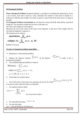
![Design and Analysis of Algorithms
Dept. of CSE, SWEC, Hyderabad Page 149
Define two functions ĉ(x) and u(x) such that for every node x,
ĉ(x) ≤ c(x) ≤ u(x)
Computing c
ˆ(·) and u(·)
Algorithm ubound ( cp, cw, k, m )
{
// Input: cp: Current profit total
// Input: cw: Current weight total
// Input: k: Index of last removed item
// Input: m: Knapsack capacity
b=cp; c=cw;
for i:=k+1 to n do{
if(c+w[i] ≤ m) then {
c:=c+w[i]; b=b-p[i];
}
}
return b;
}](https://image.slidesharecdn.com/daanotes-231027021902-07b9e3d5/85/DAA-Notes-pdf-151-320.jpg)

![Design and Analysis of Algorithms
Dept. of CSE, SWEC, Hyderabad Page 151
There are two classes of non-polynomial time problems
1. NP-Hard
2. NP-Complete
NP Complete Problem: A problem that is NP-Complete can solved in polynomial time if and only if
(iff) all other NP-Complete problems can also be solved in polynomial time.
NP-Hard: Problem can be solved in polynomial time then all NP-Complete problems can be solved in
polynomial time.
All NP-Complete problems are NP-Hard but some NP-Hard problems are not know to be
NPComplete.
Nondeterministic Algorithms:
Algorithms with the property that the result of every operation is uniquely defined are termed as
deterministic algorithms. Such algorithms agree with the way programs are executed on a computer.
Algorithms which contain operations whose outcomes are not uniquely defined but are limited to
specified set of possibilities. Such algorithms are called nondeterministic algorithms.
The machine executing such operations is allowed to choose any one of these outcomes subject to a
termination condition to be defined later.
To specify nondeterministic algorithms, there are 3 new functions.
Choice(S) arbitrarily chooses one of the elements of sets S
Failure () Signals an Unsuccessful completion Success ()
Signals a successful completion.
Example for Non Deterministic algorithms:
Algorithm Search(x){
//Problem is to search an element x
//output J, such that A[J]=x; or J=0 if x is not in A
J:=Choice(1,n); if( A[J]:=x) then {
Write(J);
Success();
}
else{ write(0);
failure();
}
Whenever there is a set of choices
that leads to a successful completion
then one such set of choices is
always made and the algorithm
terminates.
A Nondeterministic algorithm
terminates unsuccessfully if and
only if (iff) there exists no set of
choices leading to a successful
signal.](https://image.slidesharecdn.com/daanotes-231027021902-07b9e3d5/85/DAA-Notes-pdf-153-320.jpg)
![Design and Analysis of Algorithms
Dept. of CSE, SWEC, Hyderabad Page 152
Nondeterministic Knapsack algorithm
Algorithm DKP(p, w, n, m, r, x){
W:=0; P:=0; for i:=1 to n
do{ x[i]:=choice(0, 1);
W:=W+x[i]*w[i];
P:=P+x[i]*p[i];
}
if( (W>m) or (P<r) ) then Failure(); else
Success();
}
p given Profits w given
Weights
n Number of elements (number of p or w)
m Weight of bag limit
P Final Profit
W Final weight
The Classes NP-Hard & NP-Complete:
For measuring the complexity of an algorithm, we use the input length as the parameter. For example,
An algorithm A is of polynomial complexity p() such that the computing time of A is O(p(n)) for
every input of size n.
Decision problem/ Decision algorithm: Any problem for which the answer is either zero or one is
decision problem. Any algorithm for a decision problem is termed a decision algorithm.
Optimization problem/ Optimization algorithm: Any problem that involves the identification of an
optimal (either minimum or maximum) value of a given cost function is known as an optimization
problem. An optimization algorithm is used to solve an optimization problem.
P is the set of all decision problems solvable by deterministic algorithms in polynomial time.
NP is the set of all decision problems solvable by nondeterministic algorithms in polynomial time.
Since deterministic algorithms are just a special case of nondeterministic, by this we concluded that P
⊆ NP
Commonly believed relationship between P & NP
The most famous unsolvable problems in Computer Science is Whether P=NP or P≠NP In
considering this problem, s.cook formulated the following question.
If there any single problem in NP, such that if we showed it to be in ‘P’ then that would imply that
P=NP.
Cook answered this question with](https://image.slidesharecdn.com/daanotes-231027021902-07b9e3d5/85/DAA-Notes-pdf-154-320.jpg)