Numerical Investigation of Head Frontal Velocity of Non-conservative Dense Flows in Small Inclined Beds

International Research Journal of Engineering and Technology (IRJET) e-ISSN: 2395 -0056
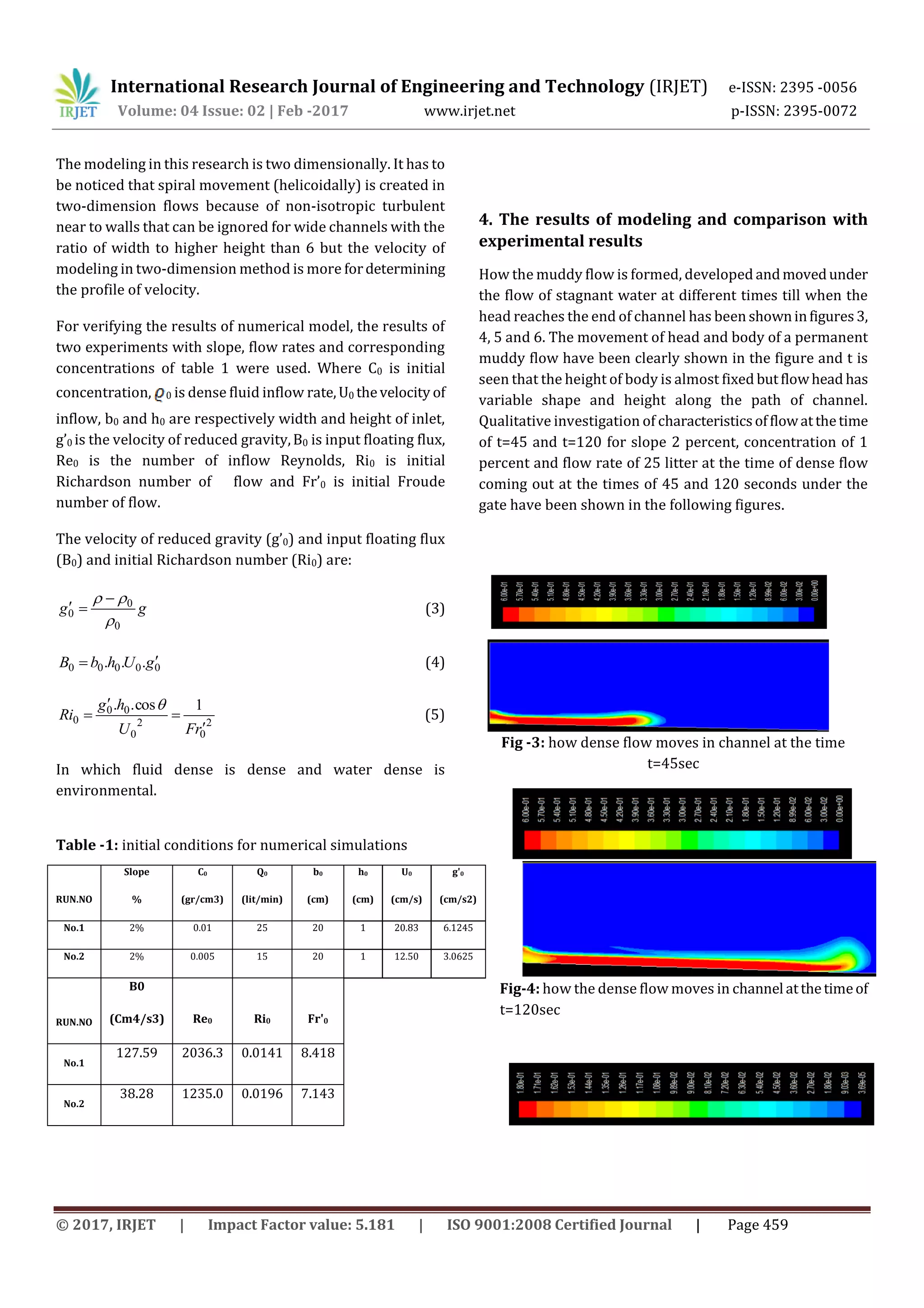
Volume: 04 Issue: 02 | Feb -2017 www.irjet.net p-ISSN: 2395-0072
© 2017, IRJET | Impact Factor value: 5.181 | ISO 9001:2008 Certified Journal | Page 457
Numerical Investigation of Head Frontal Velocity of Non-conservative
Dense Flows in Small Inclined Beds
Ehsan Hajibabaei1, Alireza Ghasmi1, Seyed Abbas Hosseini1
1Technical and Engineering Department, Science and Research Branch, Islamic Azad University, Tehran, Iran
---------------------------------------------------------------------***---------------------------------------------------------------------
Abstract - Non-conservative dense flow frontal velocityhas
been simulated two dimensionally by fluent numerical code.
The outcomes have been compared with experimental results.
Numerical simulation was conducted as two-phase through
Euler-Lagrange method. Reynolds-Stress Turbulent Model
(RSM) with non-uniform grid and shredding mesh on the
channel floor. The results obtained from numerical model of
head frontal velocity show agoodcompliance withexperiment
results and greatly help analyzing the pattern of fluid
movement in different scales.
Key Words: dense flow, fluent, head frontal velocity
1. INTRODUCTION
The specific area of head is in frontal edge of dense flow that
has been deeper than tail area and have different
characteristics of flow body. Dynamic identification of head
is very important because it is generally considered as a
boundary condition for the flow [1]. Dense flows which
stream on horizontal surface have almost semi-permanent
head and a depth twice the depth of the body of flow but in a
flow which passes on a slope, the depth of head always
increase. The shape of head in gravity flows aren’t
generalizable and severely depend on physical conditions,
environmental fluid depth and other cases. Figure (1)
represents the first experiments that are formed for
modeling the head of a cold flow of wind in atmosphere
using temperature difference. In figures (1-a) and (1-b), the
head of flow with low Reynolds numberabout10, Rer=
(Ur head velocity, hr is its height and v is kinematic viscosity)
has been shown. When temperature gets more and the
number of Reynolds increases, the form of head will change,
its nose gets closer to the earth floor and severe mix occurs
in front of and above the head. Figure (1-F) shows a flow
whose Reynolds number is upper than 1000 in which some
billows raise from high level and goes backwardly [2].
As it can be seen the head of flow is an area in which severe
disorder and turbulent happen and there is high density
gradient. When velocity and as result the number of
Reynolds in flow increase, the form of head changes and
mainly turn to more stretched mode. Whirlpool within head
during rotation generates many vortices and pollens that in
area above that breaks in three dimension and very
complicated form andcreatessomeinstabilities. Thevelocity
changes may create different types of damages such as
erosion, abrasion and cavitation which are extensively
reported for concrete and steel structures [3-5].Inheadarea
because of great vortex, turbulence and mixing and inside
mixture are also more and gradient of velocity and dense is
stronger in this area. Mixture of dense flow with fluid of
environment is an important process that occurs in head of
flow through dense fluid suction behind and back of head as
series of cross vortices [6]. Another example of turbulent
flow with hydraulic jump,vortexandpressurefluctuationsis
considered by Hamedi et al. in stepped spillways with
horizontal and inclined steps. They reported thatinclination
slightly increases the energy loss [7] Hamedi et al., also,
mentoned that the combination of inclination and end sill
increases the energy loss [8]. Also, velocity field in reservoir
has been considered by Sarkardehetal.inpresenceofan air-
core vortex as another example of turbulent flow [9].
Fig-1: The changes of radial velocity versus time
Figure 1- transformation of head of experiment gravity flow
through increasing Reynolds number a) Reynolds number
less than 10, f) Reynolds more than 1000 [2]
Using images with slow movement for tracking and
following the form of billows in upper boundary of flow
show that the wave and range of these billows can grow to
the size of head and then they are collapsed and broken [1].

2. Theoretical principles
Dominant equations on the movement of an incompressible
viscous fluid at the state of chaos are expressed using
averaged Navier-Stokes equations known as Reynolds
(RANS). Hamedi et al. mentioned all numerical models
which Fluent software is using to solve problems [10].
Continuity equation (conservation of mass) and motion
(conservation of momentum) are mentioned below [11]:
- Continuity equation
= =0 (1)
- Momentum equation
+ =- + + ( ) (2)
Ui is the component of averaged velocity in the time to the
direction of xi, p total pressure, fluid dense, gi the velocity
of gravity to the direction of xi and is stress tensorthatin
turbulent flows, it includes two terms and in addition to the
stress caused by average component of flow,theotherstress
derived from fluctuation component of velocity is created
that is known as Reynolds stresses and is shown using
Boussinesq’s idea.
Modeling in this research id conducted through Euler-
Lagrange method so that continuous phase of flow is solved
using Euler equations that are Navier-Stokes equations and
then second phase for example sedimentary particles are
investigated at the points of view of Lagrange; so that the
balance of all the forces acting on the particles in two
directions of x and y and placing them in the equation of the
size of Newton movement F=ma, give the velocity of particle
that the position of particle will be found by putting the
velocity of particle in the equation of up= that up is the
velocity of particle and xp is spatial position of particle.
Model DPM is one of capabilities of fluent in modeling two-
phase flows [12] that its second phase can be formed by
sedimentary particles or bubble or drops. Many researches
in two-phase flows have noticed this model [12].
3. Initial conditions and numerical solution of
equations
In order to solve field of flow and conducting some studies
on model, Fluent software has been used. To numerically
simulate the dominant equations on these flows, an
existing numerical code known as Fluenthas beenused.
Fluent is a strong software in the field of CFD.
Continuity and Navier-Stokes equations are used in
analyzing the flow. In case the flow is turbulent then
dominant equations turn to Reynolds ones and one-
equation, two-equation, five or six-equation modelsareused
for determining eddy viscosity thatuserdeterminesthetype
of model [11]. Fluent converts dominant equations to
algebraic equations through the method of finite volumes
and then solve them.
Considering that Fluent software doesn’t generate network
itself and the network should be generated in another
software, Fluent is capable of reading mesh from other
software such as Gambit, Geomesh and ANSIS. In this
research in first step, the shape of problem is drawn in
AutoCAD software and in the second step, meshing was
formed on general geometry in Gambit software [13],
meshing is non-uniformly and rectangular. Then the type of
the boundaries of solution zone such as wall, input and
output were specified, generated mesh is read in Fluent
software and controlled in this software in case of probable
problems such as negative volumes.
Geometry and boundary conditions of flow have been
represented in Figure 2.
Fig-2: geometry and boundary conditions of flow
For better accordance of results in the section, meshing is
fine in 20 centimeters of channel floor that whatever we get
closer to the bottom of channel, meshingwill besmaller.This
meshing method also has been used by Baqersad et al. [14]
and Hamedi and Ketabdar [15]. The configuration and
topology which was defined by Zeidi et al. [16-19] was
helpful to define mesh topology and boundary conditions.

The modeling in this research is two dimensionally. It has to
be noticed that spiral movement (helicoidally) is created in
two-dimension flows because of non-isotropic turbulent
near to walls that can be ignored for wide channels with the
ratio of width to higher height than 6 but the velocity of
modeling in two-dimension method is more fordetermining
the profile of velocity.
For verifying the results of numerical model, the results of
two experiments with slope, flow rates and corresponding
concentrations of table 1 were used. Where C0 is initial
concentration, 0 is dense fluid inflow rate,U0 thevelocity of
inflow, b0 and h0 are respectively width and height of inlet,
g’0 is the velocity of reduced gravity,B0 is input floating flux,
Re0 is the number of inflow Reynolds, Ri0 is initial
Richardson number of flow and Fr’0 is initial Froude
number of flow.
The velocity of reduced gravity (g’0) and input floating flux
(B0) and initial Richardson number (Ri0) are:
gg
0
0
0

 
 (3)
00000 ... gUhbB  (4)
2
0
2
0
00
0
1cos..
rFU
hg
Ri





(5)
In which fluid dense is dense and water dense is
environmental.
Table -1: initial conditions for numerical simulations
4. The results of modeling and comparison with
experimental results
How the muddy flow is formed, developed andmovedunder
the flow of stagnant water at different times till when the
head reaches the end of channel has been showninfigures3,
4, 5 and 6. The movement of head and body of a permanent
muddy flow have been clearly shown in the figure and t is
seen that the height of body is almost fixed butflowhead has
variable shape and height along the path of channel.
Qualitative investigation of characteristicsofflowatthetime
of t=45 and t=120 for slope 2 percent, concentration of 1
percent and flow rate of 25 litter at the time of dense flow
coming out at the times of 45 and 120 seconds under the
gate have been shown in the following figures.
Fig -3: how dense flow moves in channel at the time
t=45sec
Fig-4: how the dense flow moves in channel atthetimeof
t=120sec
RUN.NO
Slope
%
C0
(gr/cm3)
Q0
(lit/min)
b0
(cm)
h0
(cm)
U0
(cm/s)
g'0
(cm/s2)
No.1 2% 0.01 25 20 1 20.83 6.1245
No.2 2% 0.005 15 20 1 12.50 3.0625
RUN.NO
B0
(Cm4/s3) Re0 Ri0 Fr'0
No.1
127.59 2036.3 0.0141 8.418
No.2
38.28 1235.0 0.0196 7.143

Fig-5: velocity vectors of dense flows at the time t=120sec
Fig-6: velocity vectors of dense flows in head of flow
t=120sec
As following, the head frontal velocity of non-conservative
dense flows and the comparison of modeling results with
experimental results will be investigated. Being aware of
head frontal velocity in dense flows is very important in
many engineering functions. Based on this the results of
measuring velocity in head of muddy flows which have been
obtained using sound velocity meter system by previous
experimental researches [1] are used in this part.
How velocity changes, flow frontal velocity in different
distances of input using numerical model (fluent) for two
experiments have been used in figure 7. As it can be seen at
the beginning of input becauseofcreatedinstabilitiescaused
by the sudden withdrawal of dense fluid into environmental
fixed fluid, dispersion in measured velocity of fluid frontcan
be justified. In the distance about 3 meters till the end of
channel head frontal velocity is fixed. The experimental
results, obtained results of frontal velocity in flow head in
laboratory and numerical simulation (at the distance of 3 to
11 meters from channel input) have been estimated and
compared in figure 8.
In each level of numerical modeling dense flow with specific
concentration and flow rate enter the channel from one
centimeter down the hatches.Whentheflowreachesthe end
of channel, modeling will stop and considering head frontal
velocity is fixed in two-dimension flows along channel, it is
measured in middle depth of channel and then compared
with the relevant experimental results (whose
characteristics are in table 1).
Fig – 7: head frontal velocity of dense flows in different
distances of input considering obtained numerical model
(fluent)
Fig- 8: comparing the velocity of head movement of dense
flow in numerical model (fluent) with experimental results
in the distance of 3 to 11 meter from channel input

Table-2: comparing the velocity of head movementofdense
flow in numerical model (fluent) with experimental results
in the distance of 3 to 11 meter from channel input
5. Conclusion
Non-conservative dense flow frontal velocity was simulated
in this research using numerical code Fluent through Euler-
Lagrange method and was assessed as a suitable tool for
hydrodynamic simulation of behaviorofexperimental dense
flows. The comparison of modeling obtained results with
experimental results, meanwhile has verified the results of
numerical model, it has greatly helped in analyzing the
pattern of fluid movement in different scales.
1- Head frontal velocity is fixed considering numerical and
experimental modeling in two-dimension mode in
distance (3 to 11 meter) from input. Comparing the
results of numerical modeling and experimental results,
it can be observed that the results have relatively good
accordance.
2- The position of forming vortices at the time of passing
head and after that can be well observed by numerical
model. The areas with high shear stress in the center of
dense fluid with environmental fluid can be also
observed.
3- Comparing numerical model and experimental data
showed that the models of Fluent numerical code that
have been established based on CFD can give relatively
confident results and is appropriate for simulating this
type of flows. Considering the results above, analytical
models from turbulentdense flowcanbecomparedwith
empirical results of this experiment and used with
higher confidence coefficient of these models for
estimating the volume of sedimentary in channels and
reservoirs behind dam and so on.
REFERENCES
[1] A. Hosseini, “Doctoral Dissertation” Sharif University
Tehran, Iran, 2006.
[2] J. E. Simpson, “Gravity Currents in the Laboratory,
Atmosphere and Ocean”, Ann. Ev Fluid Mech., Vol.14,
1982.
[3] Champiri, M. D., Sajjadi, S., Mousavizadegan, S. H., Moodi,
F., “Assessing of Distress Cause and Estimating Evaluation
Index for Marine Concrete Structures, American Journal of
Civil Engineering and Architecture, Science and Education
Publishing, 4(4), 142-152, 2016.
[4] Champiri, M. D., Sajjadi, S., Mousavizadegan, S. H., Moodi,
F., “A Fuzzy System for Evaluation of Deteriorated Marine
Steel Structures”, Journal of Intelligent and Fuzzy Systems,
IOS press, DOI:10.3233/JIFS-161411, 2017.
[5] F. Ghasemzadeh, S. Sajedi, M. Shekarchi, & H. Layssi, M.
Hallaji, “Performanceevaluationofdifferent repairconcretes
proposed for an existing deterioratedjettystructure. Journal
of Performance of Constructed Facilities”, 28(4), 04014013,
2013.
[6] J.R.L. Allen, “Mixing at turbidity current heads and its
geological implication”, J. Sediment Petrol., No.41, 97-113,
1971.
[7] A. Hamedi, M. Ketabdar, M. Fesharaki, & A. Manoori,
“Nappe Flow Regime Energy Loss in Stepped Chutes
Equipped with Reverse Inclined Steps: Experimental
Development.” Florida Civil Engineering Journal, 2:28-37,
2016.
[8] Hamedi, A., Mansoori, A., Shamsai,A.,&Amirahmadian,S.
“ The Effect of End Sill and Stepped Slope on Stepped
Spillway Energy Dissipation.” Journal of Water Sciences
Research, 6 :1-15, 2014.
[9] H. Sarkardeh, E. Jabbari, A. R. Zarrati, S. Tavakkol,
“Velocity field in a reservoir in the presence of an air-core
vortex.”, J. Water Manage, Vol. 164, No. 4, pp. 193-200, 2013.
[10] A. Hamedi, M. Hajigholizadeh, & A. Mansoori, “Flow
Simulation and Energy Loss Estimation in the Nappe Flow
Regime of Stepped Spillways with Inclined Steps and End
Sill: A Numerical Approach.” Civil Engineering.Journal.,2(9),
426-437, 2016.
[11] FLUENT 6.3.26 User’s Guide 2008.
[12] N. Georgoulas et al, " 3D numerical modelling of
turbidity currents" Laboratory of Hydraulics and Hydraulic
Structures, Department of Civil Engineering Democritus
University of Thrace, 2010.
[13] Gambit 2.2, Tutorial Guide.
Experiment
number
DescriptionExperimentFLUENTError
No.1S2C10Q254.514.86.43
No.2S2C5Q152.662.53-4.89

[14] M. Baqersad, A. Eslami Haghighat, M. Rowshanzamir, H.
Mortazavi Bak, “Comparison of Coupled and Uncoupled
Consolidation Equations Using Finite Element Method in
Plane-Strain Condition.” Civil Engineering Journal, 2: 375-
388, 2016.
[15]Hamedi, A., Ketabdar, M. “Energy Loss Estimation and
Flow Simulation in the skimming flow Regime of Stepped
Spillways with Inclined Steps and End Sill: A Numerical
Model.” International Journal of Science and Engineering
Applications, 5(7), 399-407, 2016.
[16] Zeidi, S. M. J, Mahdi, M., “Evaluation of the physical
forces exerted on a spherical bubble inside the nozzle in a
cavitating flow with an Eulerian/Lagrangian approach”,
European journal of physics, 136(6), 2015.
[17] Zeidi, S. M. J, Mahdi, M., “Investigation effectsofinjection
pressure and compressibility and nozzle entry in diesel
injector nozzle’s flow”, journal of applied andcomputational
mechanics, 2(1), PP 83-94. ISSN: 2383-4536, 2015.
[18] Zeidi, S. M. J, Mahdi, M., “Effects of nozzle geometry and
fuel characteristics on cavitation phenomena in injection
nozzles”, The 22st Annual International Conference on
Mechanical Engineering-ISME2014, Tehran, Iran, 2014.
[19] Zeidi, S. M. J, Mahdi, M., “Investigation of viscosity effect
on velocity profile and cavitation formationindiesel injector
nozzle”, Proceedings of the 8-th International Conference on
Internal Combustion Engines, Tehran, Iran, 2014.

Numerical Investigation of Head Frontal Velocity of Non-conservative Dense Flows in Small Inclined Beds

More Related Content

What's hot

Similar to Numerical Investigation of Head Frontal Velocity of Non-conservative Dense Flows in Small Inclined Beds

More from IRJET Journal

Recently uploaded

Numerical Investigation of Head Frontal Velocity of Non-conservative Dense Flows in Small Inclined Beds