Download to read offline

![Journal of Engineering and Development, Vol. 16, No.2, June 2012 ISSN 1813- 7822
18
Subscripts
Symbol Definition Unit
j,k The Index Increment Along the Axial and Radial Direction
i Inner
o Outer
1. Introduction
Flow through circular pipes with concentric disturbed pipe has important industrial
applications in the fields of thermal and fluid engineering. Particularly its importance is noted
in process industries under particular process requirement and in the design of heat –
exchanging equipment. The associated flow patterns developed due to the presence of such
disturbed pipe can be quite complex with the development of disturbed zones and their
interactions with the confined jet. It has great influence on heat transfer effectiveness and
pumping power requirement. This clearly shows the importance of study of such flow
hydrodynamics. The model geometry is shown in figure (1). Few works have been reported
for flow disturbed by concentric circular pipes.
Mohammad [8] numerically studied the problem of steady laminar forced convection in the
entry region of concentric annuli with rotating inner walls using fluent code. Due to the axi-
symmetry of the problem, a 2D axi-symmetric model is used. Focus is on rotation number
(Ro), annulus radius ratio (N) effects on heat transfer characteristics, and the torque required
to rotate the inner walls. Air and engine oil were used in the simulation. Reynolds number
(Re) of 500 based on inlet velocity and hydraulic diameter is kept constant over the whole
range of the considered rotation numbers and radius ratios.
Mandal and Chakrabarti [7] numerically investigated disturbances of blood flow through a
stenotic coronary artery for the restrictions of 10% to 90% with the Reynolds numbers
ranging from 25 to 375. Atherosclerotic plaque formation tends to start from very low flow
Reynolds number of 25 with 50% restriction. For Reynolds numbers of 100 and above, it
starts at 30% stenosed condition. Impact of percent stenosis on wall shear stress has been
noted to be more effective than Reynolds number.
Founargiotakis et al. [3] presented an integrated approach for the flow of Herschel–Bulkley
fluids in a concentric annulus, modeled as a slot, covering the full range of flow types,
laminar, transitional, and turbulent. Prior analytical solutions for laminar flow are utilized.
Turbulent flow solutions are developed using the Metzner–Reed Reynolds number after
determining the local power law parameters as functions of flow geometry and the Herschel–
Bulkley rheological parameters. The friction factor is estimated by modifying the pipe flow
equation. Transitional flow is solved introducing transitional Reynolds numbers which are
functions of the local power law index.](https://image.slidesharecdn.com/59388c1a-bd26-44b6-96a6-c89046718b2f-160703121101/85/67504-3-320.jpg)
![Journal of Engineering and Development, Vol. 16, No.2, June 2012 ISSN 1813- 7822
19
Nam and Young [9] numerically investigated the rotating flow in an annulus. The mean
diameter of particles was 0.1 cm and a material density of 2.55 g/cm3 were used in the
experiment.
Hua-Shu et al. [4] studied integrated axial flow in an annulus between two concentric
cylinders. The critical condition for turbulent transition in annulus flow is calculated with the
energy gradient method for various radius ratios. The critical flow rate and critical Reynolds
number are given for various radius ratios. The critical condition for the instability of full-
developed laminar flow in an annulus is given following the “energy gradient method.” The
criterion for instability is based on the energy gradient method for parallel flow instability. It
is shown that the critical flow rate and the critical Reynolds number for onset of turbulent
transition increase with the radius ratio of the annulus.
The purpose of the current work is to solve the two-dimensional developing laminar flow in
the entrance and disturbed regions of concentric circular pipes for a wide range of Reynolds
number from 25 to 375.
2. Theoretcal Formulation
The mathematical analysis is presented for the Partial Differential Equations which describe
developing laminar fluid flow in concentric circular pipes. Steady, Incompressible,
Newtonian and constant property flow is assumed for developing velocity profile in the
entrance region and disturbed region of the concentric circular pipes. One other aspect of this
type model is that the velocity profile at the inlet to the main pipe is assumed to be uniform.
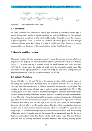
The details of the geometry under study are shown in figure(1). The flow field is determined
by solving the following equations in the computational domain using an implicit finite
difference scheme.
2.1. Governing Equations
2.1.1. Equation of Continuity:
0
)(
r
vr
z
u
r (1)
2.1.2. Equation of Momentum:
r
u
rr
u
dz
dp
r
u
v
z
u
u
11
2
2
(2)](https://image.slidesharecdn.com/59388c1a-bd26-44b6-96a6-c89046718b2f-160703121101/85/67504-4-320.jpg)
![Journal of Engineering and Development, Vol. 16, No.2, June 2012 ISSN 1813- 7822
20
2.2. Boundary Conditions
The requirement that the dependent variable or its derivative must be satisfied on the
boundary of the partial differential equation is called the boundary condition. the boundary
conditions according to the geometry will be written as follows
2.2.1. Entrance Region Boundary Conditions
Uniform velocity profile at the entrance region of main circular pipe is assumed. All entrance
boundary conditions can be written as follows [Hornbeck, 1973]:
o
o
pp
rv
uru
)0(
0),0(
),0(
(3)
2.2.1.1. Wall Boundary Conditions:
All velocity components are zero at walls, hence:
0),(
0),(
o
o
rzv
rzu
(4)
2.2.1.2. Centerline of circular pipe Boundary Conditions (symmetry line):
0)0,(
0)0,(
zv
z
r
u
(5)
2.2.2. DISturbed Region Boundary Conditions
2.2.2.1. Wall Boundary Conditions:
0),(
0),(
0),(
0),(
o
i
o
i
rzv
rzv
rzu
rzu
(6)
2.2.2.2 Centerline of circular pipe Boundary Conditions (symmetry line):
0)0,(
0)0,(
zv
z
r
u
(7)](https://image.slidesharecdn.com/59388c1a-bd26-44b6-96a6-c89046718b2f-160703121101/85/67504-5-320.jpg)
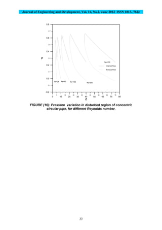
![Journal of Engineering and Development, Vol. 16, No.2, June 2012 ISSN 1813- 7822
25
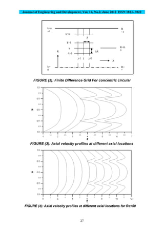
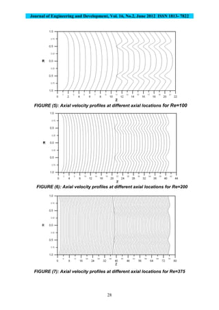
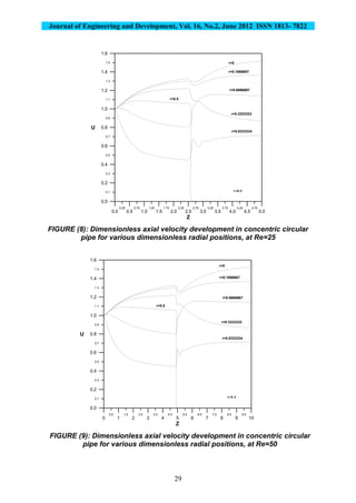
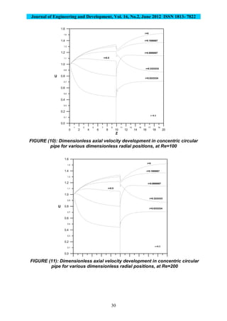
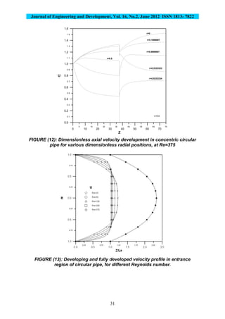
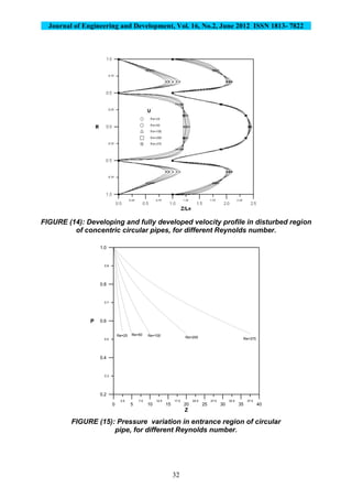
The velocity near the main pipe less than the velocity near the disturbed pipe due to the effect
of velocity at inlet annulus section. Since the volume flow rate is constant, the decrease in the
flow rate near the walls which is due to friction must be compensated by a corresponding
increase near the axis. In the entrance region the maximum velocity decreases with increasing
Reynolds number but the velocity near the wall increases with increasing Reynolds number.
The velocity profiles in fully developed is independent of Reynolds number. At a large
distance from the inlet of disturbed pipe the velocity distribution becomes parabolic. The
dimensionless pressure in the inlet section is one and decreases with increasing distance in Z-
direction due to friction. The dimensionless pressure decreases faster with the decreases of
Reynolds number. The pressure drop in annulus region is greater than pressure drop in the
inside region.
5. References
[1] Adams, J.A. and Rogers D.F. “Computer-Aided Heat Transfer Analysis”, McGraw-
Hill Book Company, New York., 1973
[2] Anderson, D.A., Tannehill, J.C., and Pletcher, R.H. “Computational Fluid Mechanics
and Heat Transfer”, McGraw-Hill Book Company, New York., 1984
[3] Founargiotakis K., Kelessidis V.C. and Maglione R. “Laminar, transitional and
turbulent flow of Herschel-Bulkley fluids in concentric annulus” , the Canadian
Journal of Chemical Engineering, Vol. 86, pp. 676-683, August 2008.
[4] Hua-Shu Dou, Boo Cheong Khoo and Her Mann Tsai “Determining the critical
condition for low transition in a full-developed annulus flow” , Journal of Petroleum
Science and Engineering, Vol. 71, 2010, in press.
[5] Hornbeck, R.W. “Numerical Marching Techniques for Fluid Flows with Heat
Transfer”, National Aeronautics and Space Administration, Washington., 1973
[6] Incropera, F.P. and Dewitt, D.P. “Fundamentals of Heat and Mass Transfer”, John
Wiley & Sons, New York., 1996
[7] Mandal D.K. and Chakrabarti S. “Two dimensional simulation of steady blood flow
through a stenosed coronary artery” , International Journal of Dynamics of Fluids,
ISSN 0973-1784, Vol. 3, No. 2, pp. 187-209, 2007.
[8] Mohammad Abdulrahman Al-Shibl “Prediction of Flow and Heat Transfer in the
Entry Region of Concentric Cylinders with Rotating Inner Walls” , M.Sc. thesis,
Mechanical Engineering Department, King Fahd University of Petroleum and
Minerals, 2006.
[9] Nam Sub Woo and Young Kyu Hwang “A Study on the Rotating Flow in an Annulus”,
International Offshore and Polar Engineering Conference Vancouver, BC, Canada,
July 6-11, 2008.](https://image.slidesharecdn.com/59388c1a-bd26-44b6-96a6-c89046718b2f-160703121101/85/67504-10-320.jpg)
![Journal of Engineering and Development, Vol. 16, No.2, June 2012 ISSN 1813- 7822
26
Table (1): Validation Data for Flow through concentric circular pipes.
Re
Pressure Gradient
[dP/dZ]
at Entrance Region
Pressure Gradient
[dP/dZ]
at Disturbed Region
Entrance Length
[Le]
present
work
AutoFEA
present
work
AutoFEA
present
work
AutoFEA
250.54810350.5380.26870640.262.52.5
500.53902690.5290.26557660.25755
1000.53500660.5250.25177390.2431010
2000.53313930.5230.2450940.2372020
3750.53230370.5220.24037650.23237.537.5
ا
Table 3: Developing Velocity Profile for Flow through concentric circular pipes
ا
R
Re=25Re=50Re=100Re=200Re=375
U(Z=1)U(Z=1)U(Z=1)U(Z=1)U(Z=1)
present
work
AutoFEA
present
work
AutoFEA
present
work
AutoFEA
present
work
AutoFEA
present
work
AutoFEA
01.2176451.221.1337341.131.0740041.071.0385491.041.0208371.02
0.16666671.209851.211.1323241.131.0738711.071.0385381.041.0208371.02
0.33333341.1768981.181.1237131.121.0725291.071.0383971.041.0208231.02
0.51.0875021.091.0870191.091.0625811.061.0364471.041.0204511.02
0.6666667.88870850.89.96138510.961.0044061.011.0155471.021.0132981.01
0.8333334.52821930.53.62869240.63.74961030.75.85179730.85.91417250.92
10000000000
1 2
δ
e
iδ
aδ
oU
Hydrodynamic entrance region Hydrodynamic disturbed region
iR
oR
eL dL
R
Z
U (R,Z)
Inviscid flow region
Boundary layer region
FIGURE (1): Laminar, hydrodynamic boundary layer development
in a concentric circular pipe.](https://image.slidesharecdn.com/59388c1a-bd26-44b6-96a6-c89046718b2f-160703121101/85/67504-11-320.jpg)

The document summarizes a numerical study of laminar flow through concentric circular pipes. The study examines developing flow in the entrance region of the main pipe and inside the disturbed pipe, where a non-uniform flow develops in the annular region around the disturbed pipe. Numerical solutions were obtained for a range of Reynolds numbers from 25 to 375 using a computer program and AutoFEA software to calculate velocity and pressure fields. Results showed the boundary layer developed faster at lower Reynolds numbers, while flow patterns were similar across cases. Findings agreed well with the AutoFEA software.


