Induced flow | Fluid Laboratory | U.O.B

SAIF AL-DIN ALI MADI
Department of Mechanical Engineering/ College of Engineering/ University of Baghdad
[Fluid Laboratory II]
University of Baghdad

TABLE OF CONTENTS
ABSTRACT.........................................................................I
OBJECTIVE........................................................................II
INTRODUCTION..............................................................V
THEORY..........................................................................VI
Calculations and results................................................VII
DISCUSSION................................................................VIII

Induced Flow
Saif Al-din Ali -B-
1. ABSTRACT
After insulating limited distance between jet hole and main
channel and find:
1. The static pressure distribution the along channel.
2. The velocity distribution on the section different dimensions.
3. The secondary flow rate discharge
4. The friction force Ff
2. OBJECTIVE
The study of the airflow generated from the pump is at a certain distance from
the cylindrical shape
3. INTRODUCTION
3.1 classification of flow:
1. Steady and unsteady flows
2. Uniform and non-uniform flows
3. One, two and three dimensional flows
4. Rotational and irrational flows
5. Laminar and turbulent flows
6. Compressible and incompressible flows

3.1.1 Steady and Unsteady Flows
Steady flow. The type of flow in which the fluid characteristics like velocity,
pressure, density, etc. at a point do not change with time is called steady flow.
Mathematically, we have:
Where (x0, y0, z0) is a fixed point in a fluid field where these variables are being measured w.r.t. time.
Example. Flow through a prismatic or non-prismatic conduit at a constant flow rate Q m3/s is
steady.
(A prismatic conduit has a constant size shape and has a velocity equation in the form u =
ax^2+
bx + c, which is independent of time t).
Unsteady flow. It is that type of flow in which the velocity, pressure or
density at a point change w.r.t. time. Mathematically, we have:
Example. The flow in a pipe whose valve is being opened or closed gradually
(velocity equation is in the form u = ax^2 + bxt).
3.1.2 Uniform and Non-uniform Flows
Uniform flow. The type of flow, in which the velocity at any given time does
not change with respect to space is called uniform flow. Mathematically, we
have:
Example. Flow through a straight prismatic conduit (i.e. flow through a straight pipe
of constant diameter).

Non-uniform flow. It is that type of flow in which the velocity at any given
time changes with respect to space. Mathematically
Example. (i) Flow through a non-prismatic conduit.
(ii) Flow around a uniform diameter pipe-bend or a canal bend
3.1.3 One, Two and Three Dimensional Flows
One dimensional flow. It is that type of flow in which the flow parameter
such as velocity is a function of time and one space co-ordinate
only. Mathematically:
u = f (x), v = 0 and w = 0
Where u, v and w are velocity components in x, y and z directions respectively
Example. Flow in a pipe where average flow parameters are considered for analysis
Two dimensional flow. The flow in which the velocity is a function
of time and two rectangular space coordinates is called two
dimensional flow. Mathematically
u = f1 (x, y) v = f2 (x, y) w = 0
Examples. (i) Flow between parallel plates of infinite extent.
(ii) Flow in the main stream of a wide river.
Three dimensional flow. It is that type of flow in
which the velocity is a function of time and three
mutually perpendicular directions. Mathematically:
u = f1 (x, y, z) v = f2 (x, y, z) w = f3 (x, y, z)
Examples.
(i) Flow in a converging or diverging pipe or channel.
(ii) Flow in a prismatic open channel in which the width and the water
Depth are of the same order of magnitude.

3.1.4 Rotational and Irrotational Flows
Rotational flow. A flow is said to be rotational if the
fluid particles while moving in the direction of flow
rotate about their mass centres. Flow near the solid
boundaries is rotational.
Example. Motion of liquid in a rotating tank.
Irrotational flow. A flow is said to be irrotational if
the fluid particles while moving in the direction of flow
do not rotate about their mass centres. Flow outside the
boundary layer is generally considered irrotational.
Example. Flow above a drain hole of a stationary tank or a
wash basin.
3.1.5 Laminar and Turbulent Flows
Laminar flow. A laminar flow is one in which paths
taken by the individual particles do not
cross one another and move along well defined paths
this type of flow is also called stream-line flow or
viscous flow.
Examples.
(i)Flow through a capillary tube.
(ii) Flow of blood in veins and arteries.
(iii) Ground water flow.
Turbulent flow. A turbulent flow is that flow in which fluid particles move
in a zig zag way
Example. High velocity flow in a conduit of large size. Nearly
all fluid flow problems encountered in engineering practice
have a turbulent character.
For Reynolds number (Re) < 2000
For Reynolds number (Re) > 4000
For Re between 2000 and 4000
... Flow in pipes is laminar.
... Flow in pipes is turbulent
... flow in pipes may be laminar or turbulent.

3.1.6 Compressible and Incompressible Flows
Compressible flow. It is that type of flow in which the
density (ρ) of the fluid changes from point to point (or in other
words density is not constant for this flow).
Mathematically: ρ ≠ constant.
Example. Flow of gases through orifices, nozzles, gas turbines, etc.
Incompressible flow. It is that type of flow in which density
is constant for the fluid flow. Liquids are generally considered
flowing incompressibly.
Mathematically: ρ = constant.
Example. Subsonic aerodynamics.
3.2 Static, Stagnation, Dynamic, Pressure
3.2.1 Static Pressure
Definition of Static pressure, or hydrostatic pressure as it is sometimes called,
is the pressure of a fluid at rest. A fluid is any substance that does not conform
to a fixed shape. This can be a liquid or a gas. Since the fluid is not moving,
static pressure is the result of the fluid's weight.
There are two different ways to measure static pressure. The first (and most
common) measure is to take the force exerted by the fluid and divide it by the
area over which it is acting. A second common method for computing static
pressure is to compute the pressure head, which is sometimes called the head,
and what you can see in the image.
Pressure Head Diagram
The pressure head is how high the fluid will go up
if the forces confining the fluid are removed.
Therefore, it has units usually associated with
length. Pressure and pressure head are
mathematically related. That relationship is
shown by these

Equations:
Dividing the pressure by the unit weight of the fluid gives us the pressure head
associated with that pressure. Unit weight (also known as specific weight) is
the weight per unit volume of fluid. This is a constant unique for each
individual fluid.
Measuring Static Pressure
Static pressure is the weight of the fluid above the point that is being
examined. To compute the pressure, use this equation (which is a
rearrangement of the pressure head equation):
The figure and the equation show that
the further you look below the surface of
the fluid the greater the hydrostatic
pressure. It's important to note that this
equation only works for
noncompressible fluids, or fluids whose
density does not change with time. This
equation will work for compressible
fluids (fluids whose density change with
time), but only over short distances

3.2.2 Dynamic pressure
Dynamic pressure (sometimes called velocity pressure) is the increase in a
moving fluid's pressure over its static value due to motion. In
incompressible fluid dynamics, it is indicated as q, or Q, defined by
Where (using SI units):
q= dynamic pressure in pascals,
p= fluid density in kg/m3 (e.g. density of water),
u= flow speed in m/s
Physical meaning
Dynamic pressure is the kinetic energy per unit volume of a fluid particle.
Dynamic pressure is in fact one of the terms of Bernoulli's equation, which can
be derived from the conservation of energy for a fluid in motion. In simplified
cases, the dynamic pressure is equal to the difference between the stagnation
pressure and the static pressure
3.2.3 stagnation pressure
The stagnation pressure, p + ρV^2/2, is the largest pressure obtainable along
a given streamline. It represents the conversion of all of the kinetic energy into
a pressure rise. The sum of the static pressure, hydrostatic pressure, and
dynamic pressure is termed the total pressure, pT. The Bernoulli equation is a
statement that the total pressure remains constant along a streamline. That is,
p + 1/2 ρV/2 + γz = pT = constant along a streamline

3.3.1 Boundary Layer Equations
In 1904, Ludwig Prandtl, the well known German scientist, introduced the
concept of boundary layer and derived the equations for boundary layer flow
by correct reduction of Navier-Stokes equations.
He hypothesized that for fluids having relatively small viscosity, the effect of
internal friction in the fluid is significant only in a narrow region surrounding
solid boundaries or bodies over which the fluid flows.
Thus, close to the body is the boundary layer where shear stresses exert an
increasingly larger effect on the fluid as one moves from free stream towards
the solid boundary.
However, outside the boundary layer where the effect of the shear stresses on
the flow is small compared to values inside the boundary layer (since the
velocity gradient is negligible),
1. The fluid particles experience no vorticity and therefore,
2. The flow is similar to a potential flow.
Hence, the surface at the boundary layer interface is a rather fictitious one,
that divides rotational and irrotational flow. Fig shows Prandtl's model
regarding boundary layer flow.
Hence with the exception of the immediate vicinity of the surface, the flow is
frictionless (inviscid) and the velocity is U (the potential velocity).
In the region, very near to the surface (in the thin layer), there is friction in the
flow which signifies that the fluid is retarded until it adheres to the surface
(no-slip condition).
The transition of the mainstream velocity from zero at the surface (with
respect to the surface) to full magnitude takes place across the boundary layer.
 u - Velocity component along x direction.
 v - velocity component along y
direction
 p - static pressure
 ρ - Density.
 μ - dynamic viscosity of the fluid

3.4 Fluid and Flow Measurements
3.4.1 MEASURING TOTAL AND STATIC PRESSURE
A tube placed in a duct facing into the
direction of the flow will measure the
total pressure in the duct. If frictional
losses are neglected, the mean total
pressure at any cross section throughout
the duct system is constant. Static pressure
can only be determined accurately by
measuring it in a manner such that the
velocity pressure has no influence on the
measurement at all. This is carried out by
measuring it through a small hole at the
wall of the duct; or a series of holes
positioned at right angles to the flow in a
surface lying parallel to the lines of flow.
The pitot static tube is an example of this.
Figure 1 shows the principle of the pitot
static tube. Figure. Principle of the pitot
static tube.
3.4.2 INSTRUMENTS FOR MEASURING PRESSURE
1. U TUBE MANOMETER.
Although probably the oldest method of measuring low
pressures, the simple U tube has much to commend it. If
a U shaped glass tube is half filled with a liquid, e.g.
water, and a pressure is applied to one end of the limb,
the other being open to atmosphere, the liquid will move
to balance the pressure. The weight of liquid so displaced
will be proportional to the pressure applied. As the
difference in height of the two columns of liquid and the
density are known the pressure can be calculated. Each
millimeter height difference of water column represents
approximately 10 Pascals.
A disadvantage of the U tube is that the scale has to be
constantly moved to
line up with the moving zero alternatively with zero taken at the centre point
the scale length is halved with subsequent loss of resolution

2. ‘LIQUID - IN GLASS’ MANOMETERS.
The disadvantages of the simple U tube manometer are overcome and other
advantages incorporated in single limb industrial manometers in which it is
only necessary to read one liquid level. In one such design, one of the limbs of
the U tube is replaced by a
reservoir, thus substantially
increasing the surface area. A
pressure applied to this reservoir
causes the level of fluid to move a
small, calculable amount. The same
volume of fluid displaced in the
glass limb produces a considerable
change in the level. This nearly
doubles the resolution compared
with the U tube manometer for
vertical instruments and gives
much greater magnification when
the limb is inclined. The
manometer fluid may be plain water, but problems can arise from algae
growing in the tube causing the density of the fluid to alter. Special blends of
paraffin are often used and these have several advantages: a free moving
meniscus, no staining of the tube, and expanded scales due to low relative
densities. Where higher pressures are required, denser fluids are used, of
which mercury is often used. For very low pressures the manometer limb is
inclined to improve the resolution further.
More precision can be achieved with adjustable - range limbs and it is
possible to achieve from 0 - 125 Pa. to 0 - 5000 Pa. with only two limbs
3. PRESSURE TRANSDUCERS.
As an alternative to the fundamental liquid - filled portable manometer,
electronic pressure transducer based instruments are available for
laboratory or site use. They are generally compact as to be hand held, and
eliminate the use of fluids, giving an acceptable level of accuracy for normal
ventilating and related air movement measurement.
The capacitance transducer employs a precision diaphragm moving between
fixed electrodes. This cause's capacitance changes proportional to a
differential pressure the piezo – resistive pressure sensor contains a silicon
chip with an integral sensing diaphragm and four piezo-resistors; pressure
applied on the diaphragm causes it to flex changing the resistance; this causes
a low level output voltage proportional to pressure. A pressure transducer -
based instrument allows continuous monitoring using a recorder, or input to
electronic storage or control equipment Microprocessor technology allows for
the pressure readings to be converted into velocity readings when using a pitot
static tube. In some instances the probe calibration factor may be inputted

separately allowing other pressure measuring probes to be used with direct
velocity readout. Several readings can be stored, with MIN, MAX and AVE
functions. In some instances, duct area can be inputted to allow direct volume
flow measurement
Pocket Manometer DB2 Airflow MEDM 5k Micro manometer
PVM100 Micro manometer

4.4.3 MEASURE VOLUME FLOW RATE
FORMULAE.
Volume flow rate = Mass flow rate / Density
Volume flow rate = Velocity x duct cross-section area
The volume flow rate in a system can be measured at the entrance to the
system, at the exit from the system, or somewhere within the system itself.
This could involve measuring the total flow rate or the flow rate in a portion
of the system. Wherever it is measured, it should be a prerequisite that the
flow should be swirl - free.
There are several methods with which the flow rate can be measured.
1. IN - LINE FLOWMETERS (STANDARD PRIMARY DEVICES)
BS1042 Part 1 : 1990 describes such devices as the venturi nozzle, the
orifice plate, and the conical inlet. The venturi nozzle and the orifice plate
may be used at the inlet to or the outlet from a system as well as between
two sections of an airway. The conical inlet draws air from a ‘free’ space at
the entrance to a system.
With regard to measuring the volume flow rate of general purpose fans, the
requirements of BS1042 with regard to the lengths of straight duct upstream
of the flow meter is reduced and BS848 Part 1 : 1980 details these changes
together with the associated uncertainty of measurement.
The general equation for these differential flowmeters is:

2. ANEMOMETER DUCT TRAVERSE.
Anemometers are instruments, which measure air velocity. Two popular
types are the Rotating vane anemometer and the Thermal anemometer. The
rotating vane type is basically a mechanical device where a shrouded
rotating vane rotates like a windmill, with delicate clockwork gearing
recording the number of revolutions of the vane on a multi - point dial.
These anemometers record the linear movement of air past the instrument
in meters or feet for as long as it is held in the airstream. By noting the time
with a stop watch the velocity in m/s or ft/min can be determined.
In more recent anemometers as each blade of the rotating vane passes a
pick up, it is ‘counted’ electronically, the signal fed into electronic circuitry
with its own time base and displays the measured velocity directly and
instantaneously without any need for external timing.
The anemometer head is normally 100 mm diameter in size, but heads as
small as 16 mm are available.
It can be used in larger ducts to traverse the duct to obtain mean duct
velocity as with the pitot - static tube.
Obviously the larger size head ( when compared to the pitot - static tube)
interferes with the airflow in smaller ducts with the result that it causes the
local duct velocity to increase to a significant effect. Figure 11 shows the
typical increase in velocity reading when placed in different sized ducts.
It is possible to have one anemometer head centrally located in its own test
duct and be independently calibrated for volume flow rate.
The Airflow 100mm rotating vane anemometers can be fitted with an
Aircone flow hood which allows the volume flow rate through small grilles to
be measured easily and accurately.
The volume flow rate can be measured using an ATP600 Airflow Measuring
Hood for larger sized grilles.
Alternatively, it is recommended that a ‘cardboard skirt’ of at least 2 x the
length of the shortest side is taped around the grille and an anemometer
traverse carried out across the entrance of the
‘cardboard skirt’ to obtain the
mean velocity.

4.4.4 DISCHARGE MEASUREMENTS
1.Orifice meter – the
simplest,
small laying-out length,
but: large losses
2. - nozzle meter
3. Venturi meter – more
complicated shape,
large laying-out length
but: small losses
Determination of discharge
• measurement: height of overflow head h under free overfall
• evaluation of discharge: corresponding equation Q = f (h)
- for standard conditions of the type of spillway, its construction and
flow conditions in approach channel ⇒ calculation of discharge
coefficient m (corresponding empirical formulae)

4. THEORY
4.1 Pressure Distribution-
Take pressure reading from manometer by using water as the liquid to the
manometer
∆hxi=ha-hxi
Where
ha; atmosphere pressure
hxi; static pressure at points (1-16)
4.2 Velocity Distribution
By using Pitot tube find the:-
Pa
2
=
pghd
103
----(1)
from the ideal gas low ;
Pa
pa
= RTa ---(2)
From eq(1)&(2) find the velocity flow :-
U = 75.1√
Ta
Pa
hd ---(3)
Where:-
hd= hs- hpito
hd= dynamic head (mm)
hs stagnation head (mm)
Ta- 25+273 (K)
hpitot= head from Pitot tube (mm)
Find the velocity flow from equation (3) at two different points the whole
tunnel one of them in laminar flow region and other in the turbulent flow
region. Draw a schematic shape velocity profile in two states above it at the
same axis

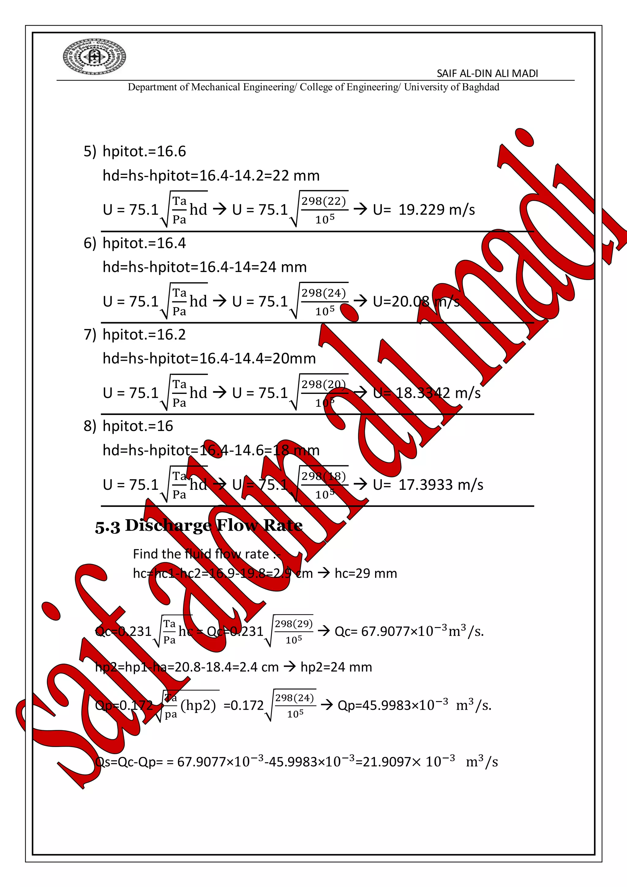
4.3 Discharge Flow Rate
Put the orifice meter in the pipe end to measurement compound flow rate
(secondary + primary), by using the following equation:
Qc = koc
𝛑𝐝𝐨𝐜 𝟐
𝟒
*75.1√
𝐓𝐚 𝐡𝐜
𝐏𝐚[𝟏−(
𝐝𝐨𝐜
𝐝
)
𝟒
]
By using available information you can obtain
Qc=0.231√
𝐓𝐚
𝐏𝐚
𝐡𝐜
Where
hc = orifice head in the end duct (mm)
The same method finds the primary flow rate (Qp):-
Qp=kop
𝛑𝐝𝐨𝐩 𝟐
𝟒
(75.1)√
𝐓𝐚
𝐏𝐚
(𝐡𝐩𝟐)
Qp=0.172√
𝐓𝐚
𝐩𝐚
(𝐡𝐩𝟐)
Where: hp orifice head in the start jet (mm).
4.4 Find the friction Force:-
1. Theoretical analysis
Re =
ρavaD
μa
μa = 1.8 × 10−5
m2
/s
ρa = 1.2 kg/m^3
F = 8TWdx
Ff = πD ∫ TW dx = πDTWl = (
π
8
1
0
)fpauc
2 Dl
Ff =
2fρa Qc
2
l
πD3

2. Experimental Analysis
This can be equal shear stress in mixed ir region (primary + conday) and shear stress
increasing maximum pressure region, the reduced pressure is found between 6 point
and 16 point
pf = ∆h = yh = ρwgh → |h16 − h6|
Experimental friction force is given by the following:-
Ff =
πD2
4
ρf
1
4
*Some number values needed during the calculations by
Kop = flow rate in primary flow (0. 595).
kot = flow rate in compound flow (0.64).
dop = diameter of the orifice in primary flow (70 min),
dn = diameter of the jet flow (35 mm),
D = diameter of the main duct (79mm).
dos = diameter of the orifice in compound flew (66mm)

5. Calculations and results
Calculations
5.1 Pressure Distribution
ha ; atmosphere pressure. =184 mm
hxi ; static pressure at points (1-16)
1- ∆hxi=ha-hxi=18.4 -18.8= - 4 mm
2- ∆hxi=ha-hxi=18.4 -18.6= - 2 mm
3- ∆hxi=ha-hxi=18.4 -16.8= 16 mm
4- ∆hxi=ha-hxi=18.4 -16.4= 20 mm
5- ∆hxi=ha-hxi=18.4 -16.2= 22 mm
6- ∆hxi=ha-hxi=18.4 -16.4= 20 mm
7- ∆hxi=ha-hxi=18.4 -16,4= 20 mm
8- ∆hxi=ha-hxi=18.4 -16.6= 18 mm
9- ∆hxi=ha-hxi=18.4 -16.6= 18 mm
10- ∆hxi=ha-hxi=18.4 -16.8= 16 mm
11- ∆hxi=ha-hxi=18.4 -16.7= 17 mm
12- ∆hxi=ha-hxi=18.4 -16.8= 16 mm
13- ∆hxi =ha-hxi=18.4 -16.8= 16 mm
14- ∆hxi=ha-hxi=18.4 -16.8= 16 mm
15- ∆hxi=ha-hxi=18.4 -16.8= 16 mm
16- ∆hxi=ha-hxi=18.4 -16.9= 15 mm

A. Turbulent Flow
1) hpitot.=18.5
hd=hs-hpitot=18.6-18.5=1mm
U = 75.1√
Ta
Pa
hd  U = 75.1√
298(1)
105
 U=4.099 m/s
2) hpitot.=18.4
hd=hs-hpitot=18.6-18.4=2 mm
U = 75.1√
Ta
Pa
hd  U = 75.1√
298(2)
105  U= 5.7977m/s
3) hpitot.=16
hd=hs-hpitot=18.6-16=26 mm
U = 75.1√
Ta
Pa
hd  U = 75.1√
298(26)
105
 U=20.9m/s
4) hpitot.=8.8
U = 75.1√
Ta
Pa
hd  U = 75.1√
298(98)
105
 U=40.5845 m/s
5) hpitot.=5.4
U = 75.1√
Ta
Pa
hd  U = 75.1√
298(133)
105  U=47.279m/s
6) hpitot.=5.7
U = 75.1√
Ta
Pa
hd  U = 75.1√
298(129)
105
 U=46.5632 m/s

7) hpitot.=12.2
U = 75.1√
Ta
Pa
hd  U = 75.1√
298(64)
105  U=32.7972m/s
8) hpitot.=17.1
U = 75.1√
Ta
Pa
hd  U = 75.1√
298(15)
105
 U= 15.877m/s
B. Laminar Flow
1) hpitot.=15.8
U = 75.1√
Ta
Pa
hd  U = 75.1√
298(8)
105
 U=11.5955 m/s
2) hpitot.=16
U = 75.1√
Ta
Pa
hd  U = 75.1√
298(14)
105  U= 15.339 m/s
3) hpitot.=16.2
hd=hs-hpitot=16.48-14.4=20.8 mm
U = 75.1√
Ta
Pa
hd  U = 75.1√
298(20.8)
105  U=18.69733m/s
4) hpitot.=16.4
U = 75.1√
Ta
Pa
hd  U = 75.1√
298 (22)
105
 U=19.229 m/s

5) hpitot.=16.6
U = 75.1√
Ta
Pa
hd  U = 75.1√
298(22)
105
 U= 19.229 m/s
6) hpitot.=16.4
U = 75.1√
Ta
Pa
hd  U = 75.1√
298(24)
105
 U=20.08 m/s
7) hpitot.=16.2
U = 75.1√
Ta
Pa
hd  U = 75.1√
298(20)
105  U= 18.3342 m/s
8) hpitot.=16
U = 75.1√
Ta
Pa
hd  U = 75.1√
298(18)
105
 U= 17.3933 m/s
5.3 Discharge Flow Rate
Find the fluid flow rate :-
hc=hc1-hc2=16.9-19.8=2.9 cm  hc=29 mm
Qc=0.231√
Ta
Pa
hc = Qc=0.231√
298(29)
105
 Qc= 67.9077×10−3m3/s.
hp2=hp1-ha=20.8-18.4=2.4 cm  hp2=24 mm
Qp=0.172√
Ta
pa
(hp2) =0.172√
298(24)
105
 Qp=45.9983×10−3 m3/s.
Qs=Qc-Qp= = 67.9077×10−3-45.9983×10−3=21.9097× 10−3 m3/s

5.4 Find the friction Force :-
1. Theoretical analysis
QC=A*Va
Va= 67.9077×10−3
/
π
4
(0.066)2
Va =19.8591 m/s
Re =
1.2∗19.8591 ∗ 0.079
1.8×10−5 = 1.0459126×105
f = 0.018
Ff =
2fρa Qc
2 l
πD3
Ff =
2(0.018) ∗ 1.2 ∗ (67.9077 × 10−3
)2
∗ 1
π 0.0793 = 12.865 × 10−3

2. Experimental Analysis
pf = ∆h = yh = ρwgh → |h16 − h6|
h = |16.9 − 16.4| = 0.005m
pf = 1000 ∗ 9.81 ∗ 0.005 = 49.05
Ff =
πD2
4
pf
1
4
Ff =
π(0.079)2
4
∗ 49.05 ∗
1
4
Ff = 60.079 × 10−3
Error=|
𝐟𝐭𝐡𝐞−𝐟 𝐞𝐱
𝐟𝐭𝐡𝐞
|*100%
1. |
𝟔𝟎.𝟎𝟕𝟗×𝟏𝟎−𝟑− 𝟏𝟐.𝟖𝟔𝟓×𝟏𝟎
−𝟑
𝟔𝟎.𝟎𝟕𝟗×𝟏𝟎−𝟑
| ∗ 𝟏𝟎𝟎% =78.586%

Results;-
5.1 Pressure Distribution
-4
-2
6
20
22
20 20
18 18
16
17
16 16 16 16
15
-10
-5
0
5
10
15
20
25
0 2 4 6 8 10 12 14 16 18
∆hxi(mm)
xi
xi
xi
Hs
(mm)
∆hxi
(mm)
1 188 -4
2 186 -2
3 168 6
4 164 20
5 162 22
6 164 20
7 164 20
8 166 18
9 166 18
10 168 16
11 167 17
12 168 16
13 168 16
14 168 16
15 168 16
16 169 15

TURBLINT LAMINAR
y hpitot hd U=m/s hpitot hd U=m/s
0 185 1 4.099 156 8 11.5955
10 184 2 5.7977 150 14 15.339
20 160 26 20.9 144 20 18.69733
30 88 98 40.5845 142 22 19.229
40 54 133 47.279 142 22 19.229
50 57 129 46.5632 140 24 20.08
60 122 64 32.797 144 20 18.334
70 171 15 15.877 146 18 17.3933
0
10
20
30
40
50
60
70
80
90
0 10 20 30 40 50 60
Y(MM)
U=M/S
TURBLINT LAMINAR

1. DISCUSSION
1.1 Draw the relation between the (∆hxi . xi) and (U, Y(radius of
the pipe)) discuss the diagram.
 the relation between the (∆hxi . xi) is mentioned above .
 the relation between (U, Y(radius of the pipe)) :-
Already answered
1.2 Derive equation (3,5 and 7)
A. equation 3
ρ = ρs + ρd
γhpito = γhs +
1
2
ρav2
1
2
ρav2 = γhpito − γhs
1
2
ρav2
= γ(hpito − hs)
∵ hd = hpito = hs
γ = ρg
1
2
ρav2
=
ρwg hd
103
− − − − − −1
PV = mRT
Ta
Pa
=
V
mR
Ta
Pa
=
L
fa R
− − − − − −2

v2 =
2pwg hd
fa 103
}/R
v2
R
=
2pwg hd
fa 103R
∵
Ta
Pa
=
1
pa
v2
R
=
2pwg hd
fa 103R
∗
Ta
𝛒 𝐚a
v = √
2 ∗ 1000 ∗ 9.81 ∗ 287
103
Ta
𝛒 𝐚
hd
v = 75.1√
Ta
𝛒 𝐚
hd
B. equation 5
Qc = kc
πdC
2
4
75.1√
Ta hc
ρa[1 − (
dC
2
D
)4]
Qc = 0.64 ∗
3.14(66 ∗ 10−3)2
4
∗ 75.1√
Ta hc
ρa[1 − (
66 ∗ 10−3
79 ∗ 10−3)4]
Qc =
0.6574
4
∗ √
Ta hc
ρa[0.5128]
Qc =
0.6574
4
∗ √
Ta hc
ρa[0.5128]
Qc =
0.6574
2.864
∗ √
Ta
ρa
hc
Qc = 0.231 ∗ √
Ta
ρa
hc

C. equation 7
QP = kP
πdP
2
4
75.1√
Ta
ρa
hP
QP = 0.64
3.14(66 ∗ 10−3)2
4
75.1√
Ta
ρa
hP
QP = 0.64
3.14(66 ∗ 10−3)2
4
75.1√
Ta
ρa
hP
Qc = 0.172√
Ta
ρa
hP
1.3 What is the main result that you have deduced from this
experimental?
First, the pressure changes along the tube between Laminar and
Turbulent and depends on several factors, including speed and
penetration.
Second, the speed increases between the center of the tube and the wall
due to friction.
1.4 Negative values appear first pressure values
Because of the pressure difference between the outside of the pipe and
the pressure of the pressure is higher than pressure inside the tube
occurs an air suction process and the values are negative at the
beginning

1.5 After calculating the experimental value of (Ffexp)
compare the calculated results with the theoretical value of
(Ffth) . than determine the percentage error between the
two values and discuss the reason of the difference
between the two values.
1. |
𝟔𝟎.𝟎𝟕𝟗×𝟏𝟎−𝟑− 𝟏𝟐.𝟖𝟔𝟓×𝟏𝟎−𝟑
𝟔𝟎.𝟎𝟕𝟗×𝟏𝟎−𝟑
| ∗ 𝟏𝟎𝟎% =78.586%
The error is due to several reasons, including the non-calibration of
the continuous device and the maintenance of the periodic
maintenance of the device and there are human errors resulting
from the inaccuracy of the readings and inaccuracy of measuring
devices used

References :-
 A TEXTBOOK OF FLUID MECHANICS AND HYDRAULIC
MACHINES
in SI UNITS Er. R.K. RAJPUT M.E. (Hons.), Gold Medallist; Grad.
(Mech.Engg. & Elect. Engg.); M.I.E. (India); M.S.E.S.I.; M.I.S.T.E.; C.E.
(India)
 fox introduction to fluid mechanics 9th ed
 Incompressible Fluids (by Dr. Ihsan Y. Hussain)

Induced flow | Fluid Laboratory | U.O.B

More Related Content

What's hot

Similar to Induced flow | Fluid Laboratory | U.O.B

More from Saif al-din ali

Recently uploaded

Induced flow | Fluid Laboratory | U.O.B