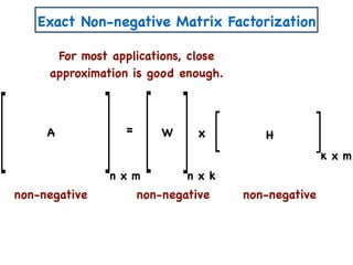
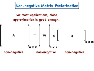
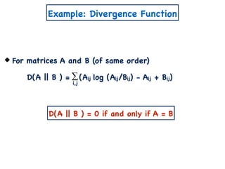
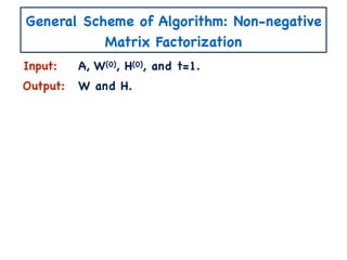
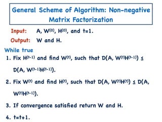
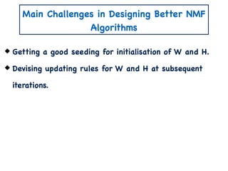
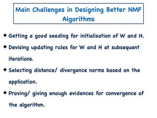
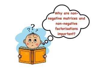
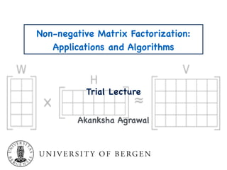
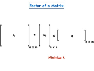
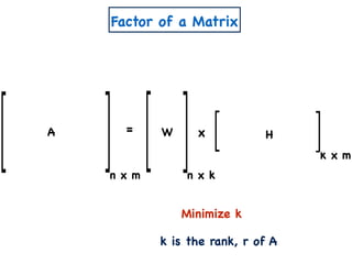
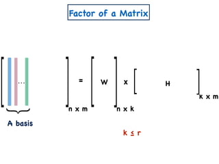
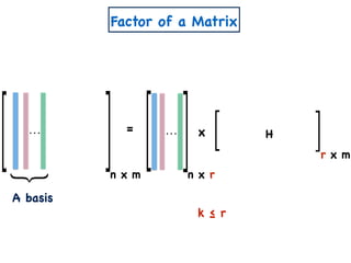
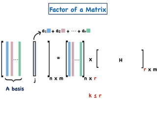
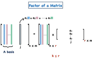
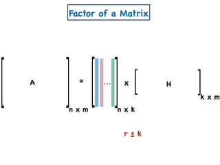
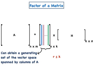
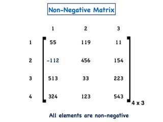
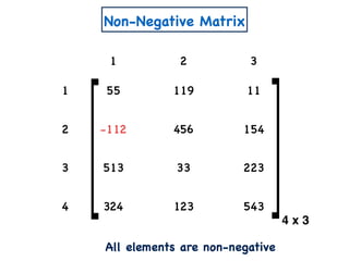
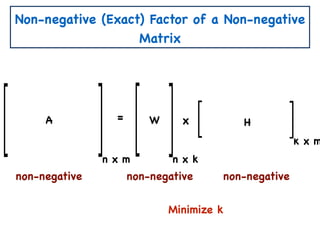
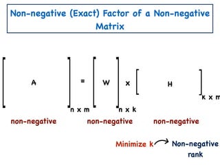
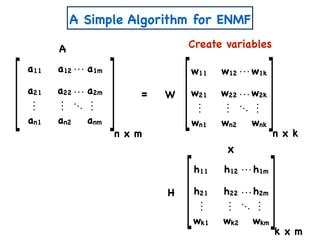
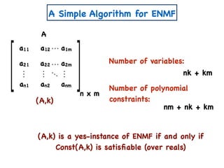
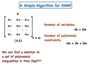
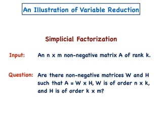
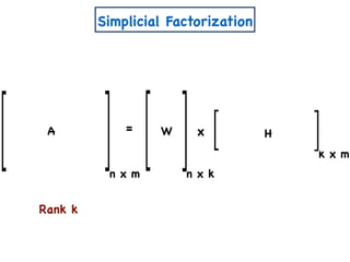
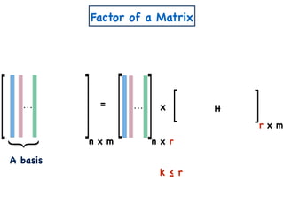
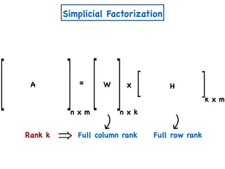
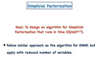
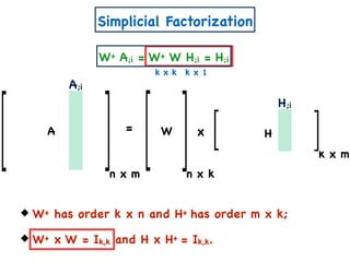
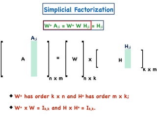
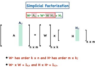
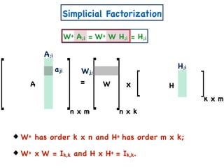
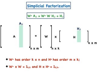
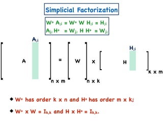
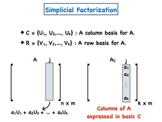
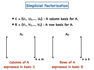
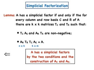
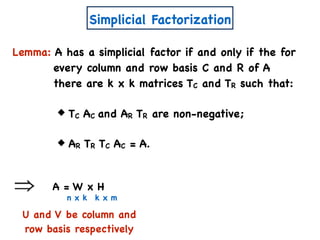
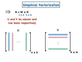
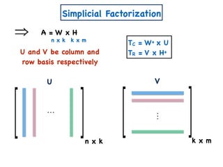
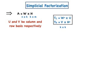
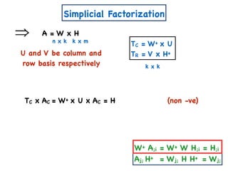
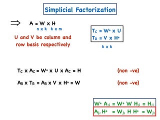
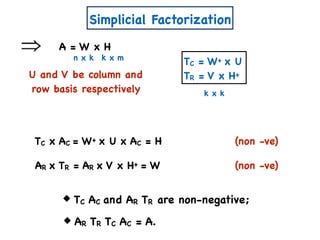
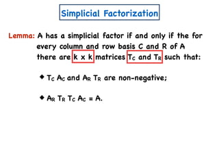
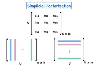
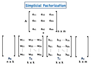
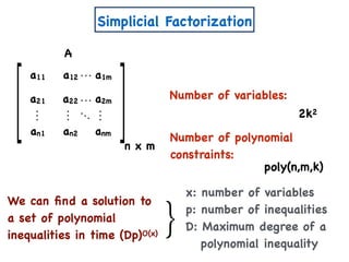
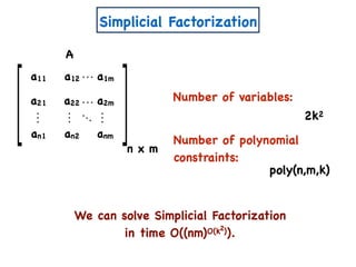
The document discusses non-negative matrix factorization and algorithms for solving it. It introduces non-negative matrix factorization as factorizing a non-negative matrix A into non-negative matrices W and H such that A = W×H. It then presents a simple algorithm for solving the exact non-negative matrix factorization problem in polynomial time by modeling it as a satisfiability problem over polynomial constraints. It also discusses an approach for simplicial factorization that reduces the number of variables by exploiting the rank of the matrix.

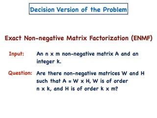
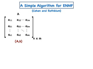
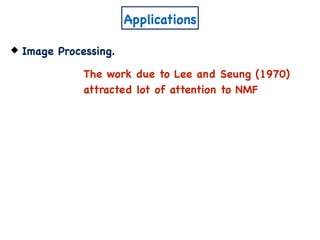
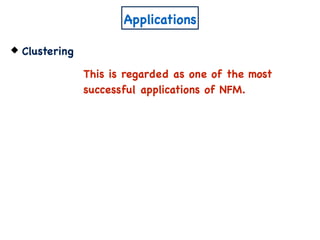
![A Simple Algorithm for ENMF
n x m
A
W
a11 a12 a1m
a21 a22 a2m
an1 an2 anm
x
n x k
w11 w12 w1k
w21 w22 w2k
wn1 wn2 wnk
k x m
h11 h12 h1m
h21 h22 h2m
wk1 wk2 wkm
Create variables
=
H
Create polynomial constraints:
[Const(A,k)]
1. For all i,j wij, hij ≥ 0.](https://image.slidesharecdn.com/trial-lecture-presentation-181003144351/85/Non-negative-Matrix-Factorization-22-320.jpg)
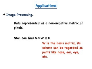
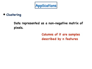
![A Simple Algorithm for ENMF
n x m
A
W
a11 a12 a1m
a21 a22 a2m
an1 an2 anm
x
n x k
w11 w12 w1k
w21 w22 w2k
wn1 wn2 wnk
H
k x m
h11 h12 h1m
h21 h22 h2m
wk1 wk2 wkm
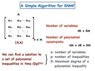
Create variables
Create polynomial constraints:
[Const(A,k)]
1. For all i,j wij, hij ≥ 0.
2. For all i,j, aij = wik hkj.∑
k
=](https://image.slidesharecdn.com/trial-lecture-presentation-181003144351/85/Non-negative-Matrix-Factorization-23-320.jpg)


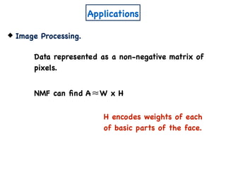
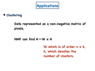
![A Simple Algorithm for ENMF
n x m
A
W
a11 a12 a1m
a21 a22 a2m
an1 an2 anm
x
n x k
w11 w12 w1k
w21 w22 w2k
wn1 wn2 wnk
H
k x m
h11 h12 h1m
h21 h22 h2m
wk1 wk2 wkm
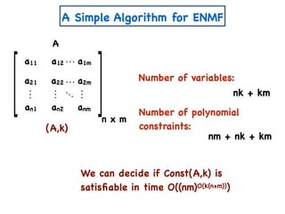
Create variables
Create polynomial constraints:
[Const(A,k)]
1. For all i,j wij, hij ≥ 0.
2. For all i,j, aij = wik hkj.∑
k
=](https://image.slidesharecdn.com/trial-lecture-presentation-181003144351/85/Non-negative-Matrix-Factorization-58-320.jpg)
![Other Results on ENMF
[Vavasis] ENMF is known to be NP-Hard.](https://image.slidesharecdn.com/trial-lecture-presentation-181003144351/85/Non-negative-Matrix-Factorization-64-320.jpg)
![Other Results on ENMF
[Vavasis] ENMF is known to be NP-Hard.
[Arora et al.] Assuming ETH, there is no algorithm for
ENMF running in time O((nm)o(k)).](https://image.slidesharecdn.com/trial-lecture-presentation-181003144351/85/Non-negative-Matrix-Factorization-65-320.jpg)
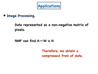
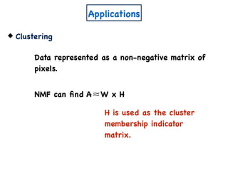
![Other Results on ENMF
2
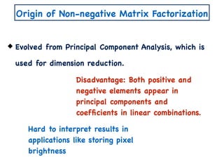
[Vavasis] ENMF is known to be NP-Hard.
[Arora et al.] Assuming ETH, there is no algorithm for
ENMF running in time O((nm)o(k)).
[Moitra] EMNF admits an algorithm running in time
O((nm)O(k )).](https://image.slidesharecdn.com/trial-lecture-presentation-181003144351/85/Non-negative-Matrix-Factorization-66-320.jpg)