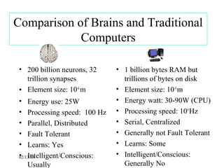
This document provides an introduction to neural networks. It discusses what connectionist neural networks are, including their key components of nodes, connections between nodes, distributed information storage, and learning through gradual changes in connection strength. The document then covers the history of neural networks, biological inspiration from the brain, different types of neural networks like perceptrons and backpropagation networks, and learning algorithms like LMS and unsupervised learning techniques like Hopfield networks and self-organizing maps.

1. Introduction to Neural Networks
By. Ruchi Sharma
BVCOE
DELHI
02/13/13

2. What are connectionist neural
networks?
• Connectionism refers to a computer modeling
approach to computation that is loosely based
upon the architecture of the brain.
• Many different models, but all include:
– Multiple, individual “nodes” or “units” that operate at
the same time (in parallel)
– A network that connects the nodes together
– Information is stored in a distributed fashion among the
links that connect the nodes
– Learning can occur with gradual changes in connection
strength
02/13/13

3. Neural Network History
• History traces back to the 50’s but became popular in the 80’s
with work by Rumelhart, Hinton, and Mclelland
– A General Framework for Parallel Distributed Processing in Parallel
Distributed Processing: Explorations in the Microstructure of
Cognition
• Peaked in the 90’s. Today:
– Hundreds of variants
– Less a model of the actual brain than a useful tool, but still some
debate
• Numerous applications
– Handwriting, face, speech recognition
– Vehicles that drive themselves
– Models of reading, sentence production, dreaming
• Debate for philosophers and cognitive scientists
– Can human consciousness or cognitive abilities be explained by a
connectionist model or does it require the manipulation of symbols?
02/13/13

4. Comparison of Brains and Traditional
Computers
• 200 billion neurons, 32 • 1 billion bytes RAM but
trillion synapses trillions of bytes on disk
• Element size: 10-6 m • Element size: 10-9 m
• Energy use: 25W • Energy watt: 30-90W (CPU)
• Processing speed: 100 Hz • Processing speed: 109 Hz
• Parallel, Distributed • Serial, Centralized
• Fault Tolerant • Generally not Fault Tolerant
• Learns: Yes • Learns: Some
• Intelligent/Conscious:
02/13/13
• Intelligent/Conscious:
Usually Generally No

5. Biological Inspiration
Idea : To make the computer more robust, intelligent, and learn, …
Let’s model our computer software (and/or hardware) after the brain
“My brain: It's my second favorite organ.”
- Woody Allen, from the movie Sleeper
02/13/13

6. Neurons in the Brain
• Although heterogeneous, at a low level
the brain is composed of neurons
– A neuron receives input from other neurons
(generally thousands) from its synapses
– Inputs are approximately summed
– When the input exceeds a threshold the neuron
sends an electrical spike that travels that
travels from the body, down the axon, to the
next neuron(s)
02/13/13

7. Learning in the Brain
• Brains learn
– Altering strength between neurons
– Creating/deleting connections
• Hebb’s Postulate (Hebbian Learning)
– When an axon of cell A is near enough to excite a cell B and repeatedly
or persistently takes part in firing it, some growth process or metabolic
change takes place in one or both cells such that A's efficiency, as one
of the cells firing B, is increased.
• Long Term Potentiation (LTP)
– Cellular basis for learning and memory
– LTP is the long-lasting strengthening of the connection between two
nerve cells in response to stimulation
– Discovered in many regions of the cortex
02/13/13

8. Perceptrons
• Initial proposal of connectionist networks
• Rosenblatt, 50’s and 60’s
• Essentially a linear discriminant composed of
nodes, weights
I1 W1 I1 W1
or
I2 W2 θ O I2 W2 O
W3 W3
I3 Activation Function I3
 
O=  i
 
1 :  ∑ wi I i  + θ > 0

θ

02/13/13  0 : otherwise  1
 

9. Perceptron Example
2 .5
1 .3 θ =-1
2(0.5) + 1(0.3) + -1 = 0.3 , O=1
Learning Procedure:
Randomly assign weights (between 0-1)
Present inputs from training data
Get output O, nudge weights to gives results toward our
desired output T
Repeat; stop when no errors, or enough epochs completed
02/13/13

10. Perception Training
wi (t + 1) = wi (t ) + ∆wi (t )
∆wi (t ) = (T − O ) I i
Weights include Threshold. T=Desired, O=Actual output.
Example: T=0, O=1, W1=0.5, W2=0.3, I1=2, I2=1,Theta=-1
w1 (t + 1) = 0.5 + (0 − 1)( 2) = −1.5
w2 (t + 1) = 0.3 + (0 − 1)(1) = −0.7
wθ (t + 1) = −1 + (0 − 1)(1) = −2
If we present this input again, we’d output 0 instead
02/13/13

11. How might you use a perceptron
network?
• This (and other networks) are generally used to learn how
to make classifications
• Say you have collected some data regarding the diagnosis
of patients with heart disease
– Age, Sex, Chest Pain Type, Resting BPS, Cholesterol, …,
Diagnosis (<50% diameter narrowing, >50% diameter narrowing)
– 67,1,4,120,229,…, 1
– 37,1,3,130,250,… ,0
– 41,0,2,130,204,… ,0
• Train network to predict heart disease of new patient
02/13/13

12. Perceptrons
• Can add learning rate to speed up the learning process; just
multiply in with delta computation
• Essentially a linear discriminant
• Perceptron theorem: If a linear discriminant exists that can
separate the classes without error, the training procedure is
guaranteed to find that line or plane.
Class1 Class2
02/13/13

13. Exclusive Or (XOR) Problem
1 0
Input: 0,0 Output: 0
Input: 0,1 Output: 1
Input: 1,0 Output: 1
Input: 1,1 Output: 0
0 1
XOR Problem: Not Linearly Separable!
We could however construct multiple layers of perceptrons to get around
02/13/13
this problem. A typical multi-layered system minimizes LMS Error,

14. LMS Learning
LMS = Least Mean Square learning Systems, more general than the
previous perceptron learning rule. The concept is to minimize the total
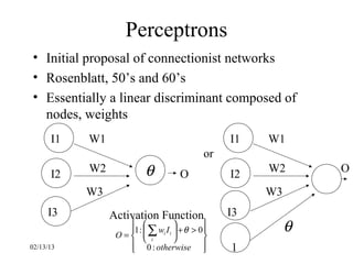
error, as measured over all training examples, P. O is the raw output,
as calculated by ∑ wi I i + θ
i
1
Dis tan ce( LMS ) = ∑ ( TP − OP )
2
2 P
E.g. if we have two patterns and
T1=1, O1=0.8, T2=0, O2=0.5 then D=(0.5)[(1-0.8) 2+(0-0.5)2]=.145
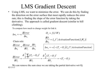
We want to minimize the LMS:
C-learning rate
E W(old)
W(new)
02/13/13
W

15. LMS Gradient Descent
• Using LMS, we want to minimize the error. We can do this by finding
the direction on the error surface that most rapidly reduces the error
rate; this is finding the slope of the error function by taking the
derivative. The approach is called gradient descent (similar to hill
climbing).
To compute how much to change weight for link k:
δError Oj = f (I W )
∆wk = − c
δwk
δO j
= I k f ' ( ActivationFunction ( I kWk ) )
Chain rule: δwk
δError δError δO j
δwk
=
δO j
∗
δwk ∆wk = −c ( − (T j − O j ) ) I k f ' ( ActivationFunction )
1
δ ∑ (TP − OP ) 2 δ 1 (T j − O j ) 2
δError 2 P
= = 2 = −(T j − O j )
δO j δO j δO j
We can remove the sum since we are taking the partial derivative wrt Oj
02/13/13

16. Activation Function
• To apply the LMS learning rule, also
known as the delta rule, we need a
differentiable activation function.
∆wk = cI k (T j − O j ) f ' ( ActivationFunction )
Old: New:
1 : ∑ wi I i + θ > 0
  O=
1
O= i  − ∑ wi I i + Θ
 0 : otherwise 
  1+ e i
02/13/13
−θ

17. LMS vs. Limiting Threshold
• With the new sigmoidal function that is differentiable, we
can apply the delta rule toward learning.
• Perceptron Method
– Forced output to 0 or 1, while LMS uses the net output
– Guaranteed to separate, if no error and is linearly separable
• Otherwise it may not converge
• Gradient Descent Method:
– May oscillate and not converge
– May converge to wrong answer
– Will converge to some minimum even if the classes are not
linearly separable, unlike the earlier perceptron training method
02/13/13

18. Backpropagation Networks
• Attributed to Rumelhart and McClelland, late 70’s
• To bypass the linear classification problem, we can
construct multilayer networks. Typically we have fully
connected, feedforward networks.
Input Layer Hidden Layer Output Layer
I1 O1
H1
I2 1
O( x) = −∑ w j , x H j
H2 O2 1+ e j
I3
Wi,j 1 Wj,k 1
1 H ( x) = − ∑ wi , x I i
1+ e i
1’s - bias
02/13/13

19. Backprop - Learning
Learning Procedure:
Randomly assign weights (between 0-1)
Present inputs from training data, propagate to outputs
Compute outputs O, adjust weights according to the delta
rule, backpropagating the errors. The weights will be
nudged closer so that the network learns to give the
desired output.
Repeat; stop when no errors, or enough epochs completed
02/13/13

20. Backprop - Modifying Weights
We had computed:
∆wk = cI k (T j − O j ) f ' ( ActivationFunction ) ;
 1 
f = −sum 
1+ e 
∆wk = cI k ( T j − O j ) ( f ( sum )(1 − f ( sum) )
For the Output unit k, f(sum)=O(k). For the output units, this is:
∆w j ,k = cH j ( Tk − Ok ) Ok (1 − Ok )
For the Hidden units (skipping some math), this is:
∆wi , j = cH j (1 − H j ) I i ∑ (Tk − Ok )Ok (1 − Ok )w j ,k
k
I H O
02/13/13 Wi,j Wj,k

21. Backprop
• Very powerful - can learn any function, given enough
hidden units! With enough hidden units, we can generate
any function.
• Have the same problems of Generalization vs.
Memorization. With too many units, we will tend to
memorize the input and not generalize well. Some schemes
exist to “prune” the neural network.
• Networks require extensive training, many parameters to
fiddle with. Can be extremely slow to train. May also fall
into local minima.
• Inherently parallel algorithm, ideal for multiprocessor
hardware.
• Despite the cons, a very powerful algorithm that has seen
widespread successful deployment.
02/13/13

22. Backprop Demo
• QwikNet
– Learning XOR, Sin/Cos functions
02/13/13

23. Unsupervised Learning
• We just discussed a form of supervised learning
– A “teacher” tells the network what the correct output is
based on the input until the network learns the target
concept
• We can also train networks where there is no
teacher. This is called unsupervised learning.
The network learns a prototype based on the
distribution of patterns in the training data. Such
networks allow us to:
– Discover underlying structure of the data
– Encode or compress the data
– Transform the data
02/13/13

24. Unsupervised Learning – Hopfield
Networks
• A Hopfield network is a type of content-
addressable memory
– Non-linear system with attractor points that
represent concepts
– Given a fuzzy input the system converges to the
nearest attractor
• Possibility to have “spurious” attractors that is a blend
of multiple stored patterns
• Also possible to have chaotic patterns that never
converge
02/13/13

25. Standard Binary Hopfield Network
• Recurrent; Every unit is connected to every other unit
• Weights connecting units are symmetrical
– wij = wji
• If the weighted sum of the inputs exceeds a threshold, its
output is 1 otherwise its output is -1
• Units update themselves asynchronously as their inputs
change A
wAD
wAB
wAC
B
wBC wBD
C D
02/13/13
wCD

26. Hopfield Memories
• Setting the weights:
– A pattern is a setting of on or off for each unit
– Given a set of Q patterns to store
• For every weight connecting units i and j:
Q
wij = ∑ xip x jp
p =1
• This is a form of a Hebbian rule which makes the weight
strength proportional to the product of the firing rates of the
two interconnected units
02/13/13

27. Hopfield Network Demo
• http://www.cbu.edu/~pong/ai/hopfield/hopfieldap
plet.html
• Properties
– Settles into a minimal energy state
– Storage capacity low, only 13% of number of units
– Can retrieve information even in the presence of noisy
data, similar to associative memory of humans
02/13/13

28. Unsupervised Learning – Self
Organizing Maps
• Self-organizing maps (SOMs) are a data
visualization technique invented by Professor
Teuvo Kohonen
– Also called Kohonen Networks, Competitive Learning,
Winner-Take-All Learning
– Generally reduces the dimensions of data through the
use of self-organizing neural networks
– Useful for data visualization; humans cannot visualize
high dimensional data so this is often a useful technique
to make sense of large data sets
02/13/13

29. Basic “Winner Take All” Network
• Two layer network
– Input units, output units, each input unit is connected to each
output unit
Input Layer Output Layer
I1 O1
I2
O2
I3
Wi,j
02/13/13

30. Basic Algorithm
– Initialize Map (randomly assign weights)
– Loop over training examples
• Assign input unit values according to the values in the current
example
• Find the “winner”, i.e. the output unit that most closely
matches the input units, using some distance metric, e.g.
For all output units j=1 to m 2
∑ (W − Ii )
n
and input units i=1 to n
ij
Find the one that minimizes: i =1
• Modify weights on the winner to more closely match the input
∆W t +1 = c( X it − W t )
where c is a small positive learning constant
02/13/13 that usually decreases as the learning proceeds

31. Result of Algorithm
• Initially, some output nodes will randomly be a
little closer to some particular type of input
• These nodes become “winners” and the weights
move them even closer to the inputs
• Over time nodes in the output become
representative prototypes for examples in the input
• Note there is no supervised training here
• Classification:
– Given new input, the class is the output node that is the
winner
02/13/13

32. Typical Usage: 2D Feature Map
• In typical usage the output nodes form a 2D “map”
organized in a grid-like fashion and we update weights in a
neighborhood around the winner
Output Layers
Input Layer
O11 O12 O13 O14 O15
I1
O21 O22 O23 O24 O25
I2 O31 O32 O33 O34 O35
… O41 O42 O43 O44 O45
I3 O51 O52 O53 O54 O55
02/13/13

33. Modified Algorithm
– Initialize Map (randomly assign weights)
– Loop over training examples
• Assign input unit values according to the values in the current
example
• Find the “winner”, i.e. the output unit that most closely
matches the input units, using some distance metric, e.g.
• Modify weights on the winner to more closely match the input
• Modify weights in a neighborhood around the winner so
the neighbors on the 2D map also become closer to the
input
– Over time this will tend to cluster similar items closer on the
map
02/13/13

34. Updating the Neighborhood
• Node O44 is the winner
– Color indicates scaling to update neighbors
Output Layers
∆W t +1 = c( X it − W t )
O11 O12 O13 O14 O15
O21 O22 O23 O24 O25 c=1 Consider if O42
is winner for
O31 O32 O33 O34 O35
c=0.75
some other
O41 O42 O43 O44 O45
c=0.5 input; “fight”
O51 O52 O53 O54 O55 over claiming
02/13/13
O43, O33, O53

35. Selecting the Neighborhood
• Typically, a “Sombrero Function” or Gaussian
function is used
• Neighborhood size usually decreases over time to
allow initial “jockeying for position” and then
“fine-tuning” as algorithm proceeds
02/13/13

36. Color Example
• http://davis.wpi.edu/~matt/courses/soms/ap
plet.html
02/13/13

37. Kohonen Network Examples
• Document Map:
http://websom.hut.fi/websom/milliondemo/
html/root.html
02/13/13

38. Poverty Map
http://www.cis.hut.fi/rese
arch/som-
research/worldmap.html
02/13/13

39. SOM for Classification
• A generated map can also be used for classification
• Human can assign a class to a data point, or use the
strongest weight as the prototype for the data point
• For a new test case, calculate the winning node and
classify it as the class it is closest to
• Handwriting recognition example: http://fbim.fh-
regensburg.de/~saj39122/begrolu/kohonen.html
02/13/13

40. Psychological and Biological
Considerations of Neural Networks
• Psychological
– Neural network models learn, exhibit some behavior similar to
humans, based loosely on brains
– Create their own algorithms instead of being explicitly programmed
– Operate under noisy data
– Fault tolerant and graceful degradation
– Knowledge is distributed, yet still some localization
• Lashley’s search for engrams
• Biological
– Learning in the visual cortex shortly after birth seems to correlate
with the pattern discrimination that emerges from Kohonen Networks
– Criticisms of the mechanism to update weights; mathematically
driven; feedforward supervised network unrealistic
02/13/13

41. Connectionism
• What’s hard for neural networks? Activities beyond
recognition, e.g.:
– Variable binding
– Recursion
– Reflection
– Structured representations
• Connectionist and Symbolic Models
– The Central Paradox of Cognition (Smolensky et al., 1992):
– "Formal theories of logical reasoning, grammar, and other higher
mental faculties compel us to think of the mind as a machine for rule-
based manipulation of highly structured arrays of symbols. What we
know of the brain compels us to think of human information
processing in terms of manipulation of a large unstructured set of
numbers, the activity levels of interconnected neurons. Finally, the full
richness of human behavior, both in everyday environments and in the
controlled environments of the psychological laboratory, seems to defy
rule-based description, displaying strong sensitivity to subtle statistical
factors in experience, as well as to structural properties of information.
To solve the Central Paradox of Cognition is to resolve these
contradictions with a unified theory of the organization of the mind, of
02/13/13
the brain, of behavior, and of the environment."

42. Possible Relationships?
• Symbolic systems implemented via
connectionism
– Possible to create hierarchies of networks with
subnetworks to implement symbolic systems
• Hybrid model
– System consists of two separate components;
low-level tasks via connectionism, high-level
tasks via symbols
02/13/13

43. Proposed Hierarchical Model
• Jeff Hawkins
• Founder: Palm Computing, Handspring
• Deep interest in the brain all his life
• Book: “On Intelligence”
– Variety of neuroscience research as input
– Includes his own ideas, theories, guesses
– Increasingly accepted view of the brain
02/13/13

44. The Cortex
• Hawkins’s point of interest in the brain
– “Where the magic happens”
• Hierarchically-arranged in regions
• Communication up the hierarchy
– Regions classify patterns of their inputs
– Regions output a ‘named’ pattern up the hierarchy
• Communication down the hierarchy
– A high-level region has made a prediction
– Alerts lower-level regions what to expect
02/13/13

45. Hawkins Quotes
“The human cortex is particularly large and
therefore has a massive memory capacity.
It is constantly predicting what you will see,
hear and feel, mostly in ways you are
unconscious of. These predictions are our
thoughts, and when combined with sensory
inputs, they are our perceptions. I call this
view of the brain the memory-prediction
framework of intelligence.”
02/13/13

46. Hawkins Quotes
“Your brain constantly makes predictions
about the very fabric of the world we live
in, and it does so in a parallel fashion. It
will just as readily detect an odd texture, a
misshapen nose, or an unusual motion. It
isn’t obvious how pervasive these mostly
unconscious predictions are, which is
perhaps why we missed their importance.”
02/13/13

47. Hawkins Quotes
“Your brain constantly makes predictions
about the very fabric of the world we live
in, and it does so in a parallel fashion. It
will just as readily detect an odd texture, a
misshapen nose, or an unusual motion. It
isn’t obvious how pervasive these mostly
unconscious predictions are, which is
perhaps why we missed their importance.”
02/13/13

48. Hawkins Quotes
“Suppose when you are out, I sneak over to
your home and change something about
your door. It could be almost anything. I
could move the knob over by and inch,
change a round knob into a thumb latch, or
turn it from brass to chrome…. When you
come home that day and attempt to open the
door, you will quickly detect that
something is wrong.”
02/13/13

49. Prediction
• Prediction means that the neurons involved
in sensing your door become active in
advance of them actually receiving sensory
input.
– When the sensory input does arrive, it is
compared with what is expected.
– Two way communication; classification up the
hierarchy, prediction down the hierarchy
02/13/13

50. Prediction
• Prediction is not limited to patterns of low-level
sensory information like hearing and seeing
• Mountcastle’s principle : we have lots of
different neurons, but they basically do the
same thing (particularly in the neocortex)
– What is true of low-level sensory areas must be true
for all cortical areas. The human brain is more
intelligent than that of other animals because it can
make predictions about more abstract kinds of
patterns and longer temporal pattern sequences.”
02/13/13

51. Visual Hierarchies
• Lowest visual level inputs pixels
• Second level recognizes edges, lines, etc
from known patterns of pixels
• Third level recognizes shapes from known
patterns of edges, lines, etc
• Fourth level recognizes objects from known
patterns of shapes
02/13/13

52. Layers
02/13/13

53. Not there yet…
• Many issues remain to be addressed by
Hawkins’ model
– Missing lots of details on how his model could
be implemented in a computer
– Creativity?
– Evolution?
– Planning?
– Rest of the brain, not just neocortex?
02/13/13