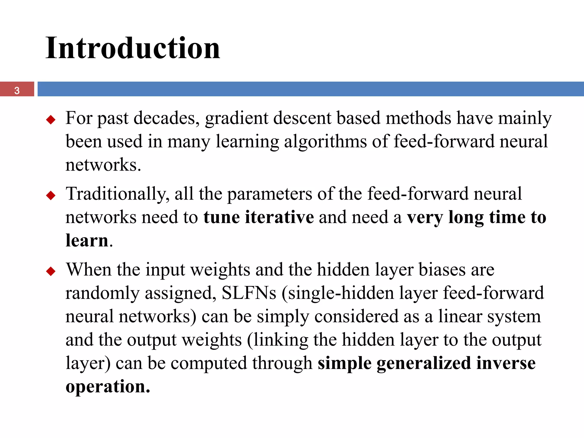
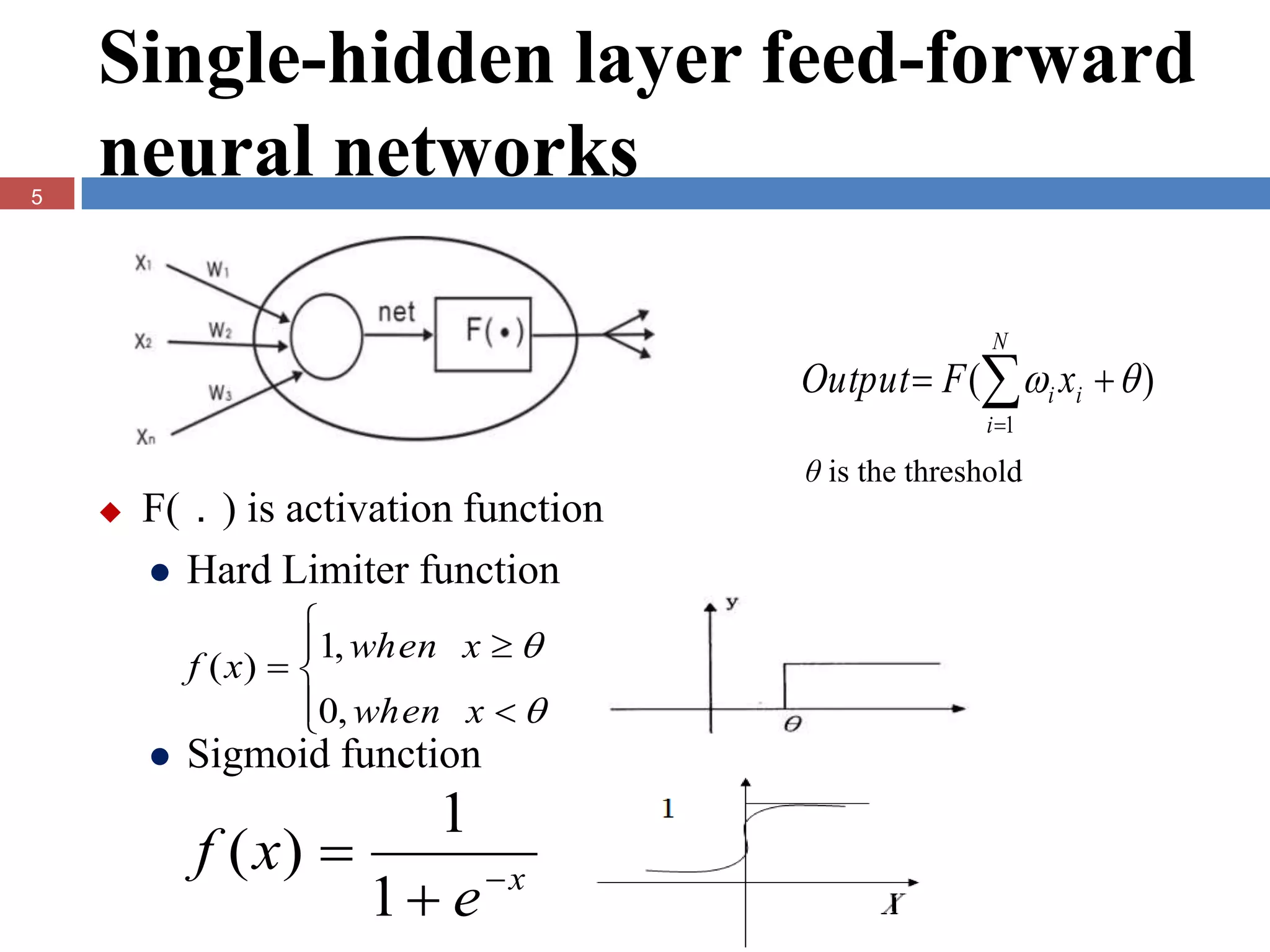
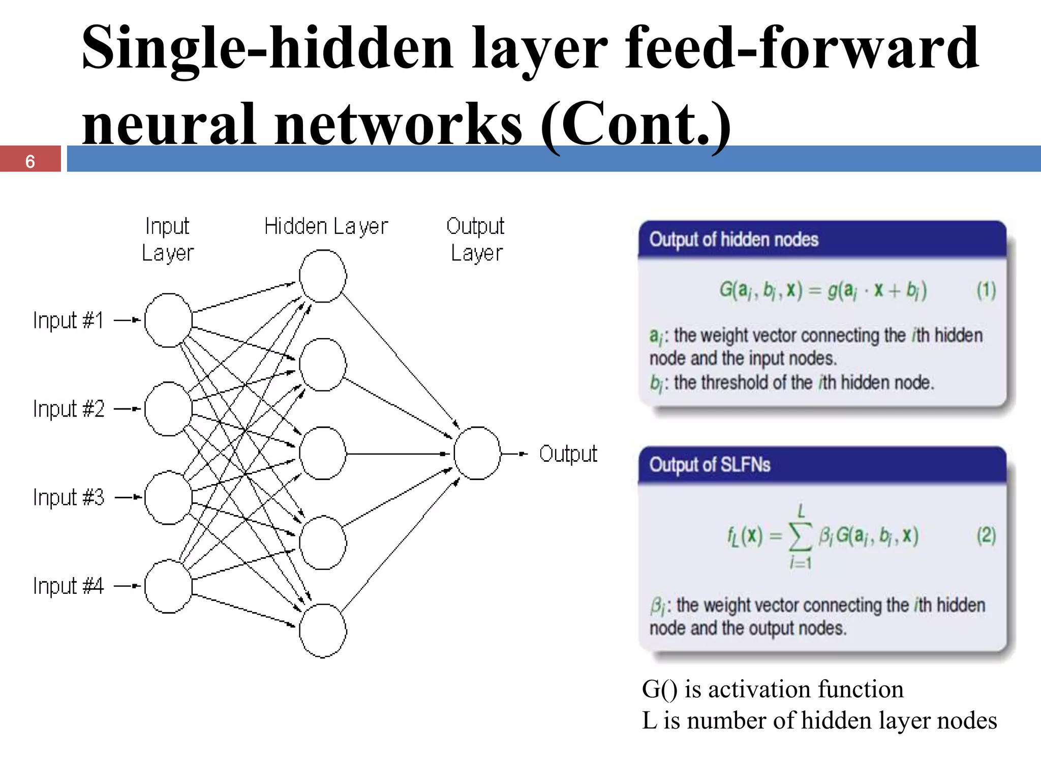
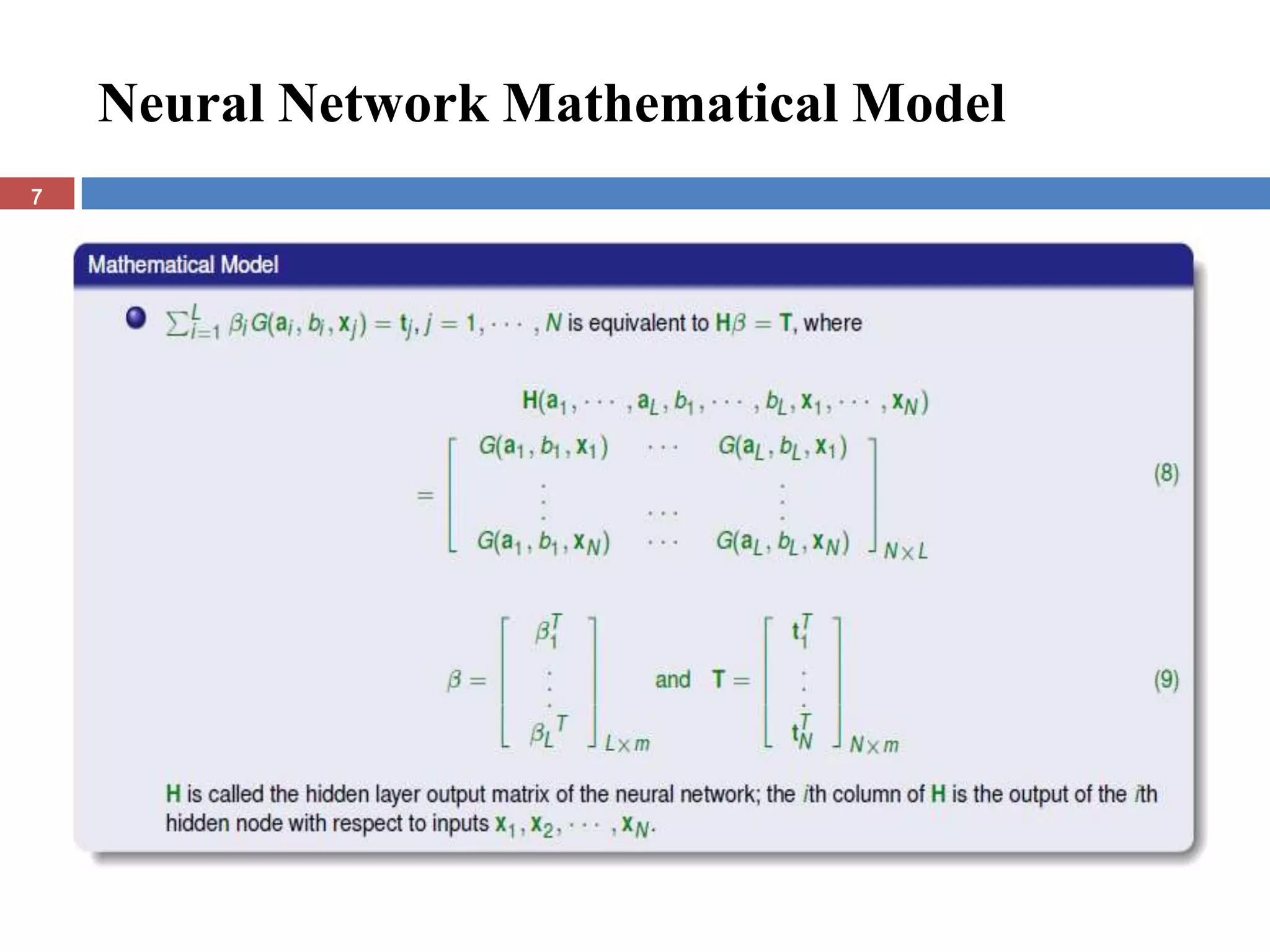
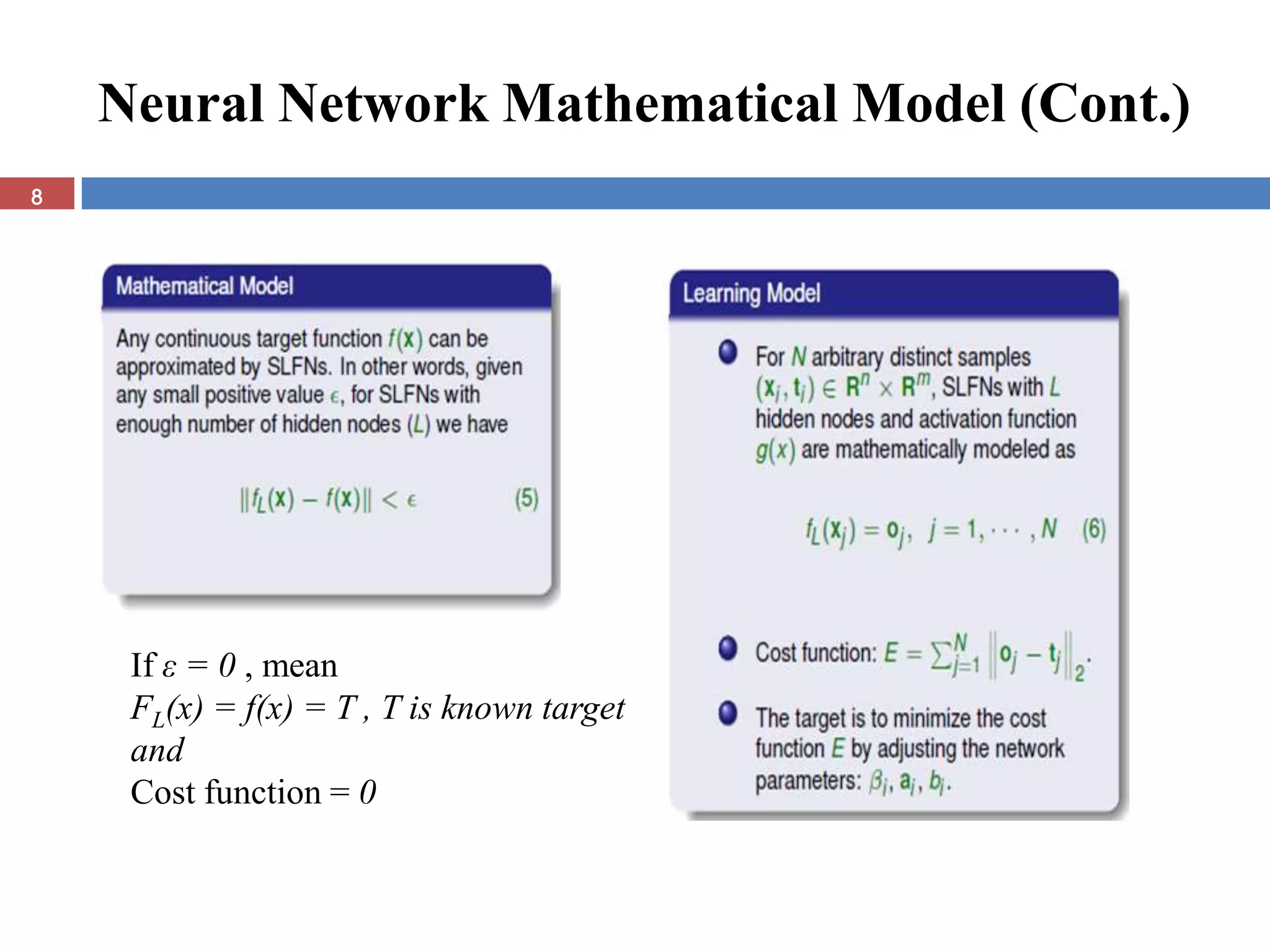
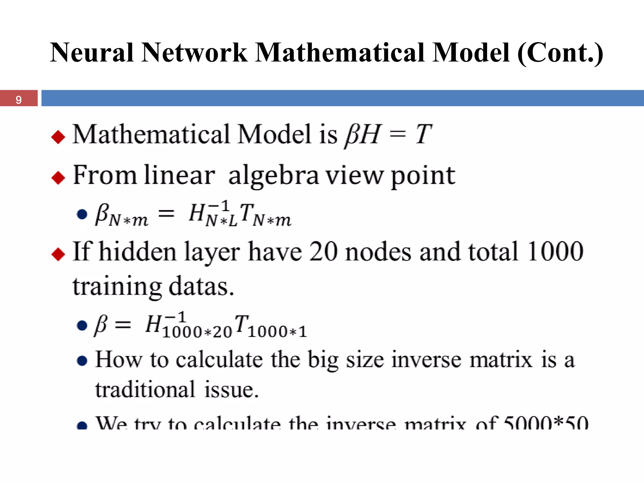
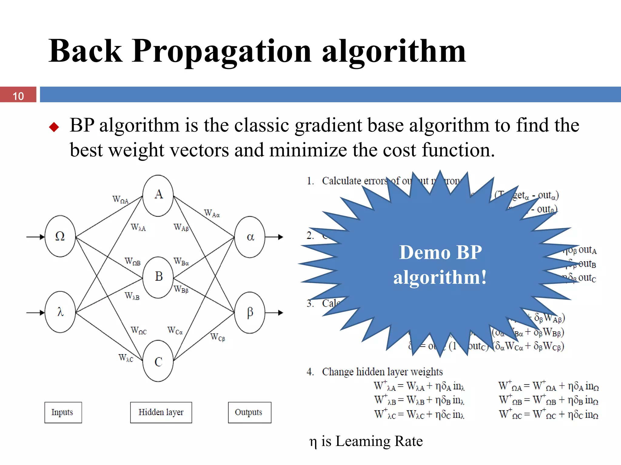
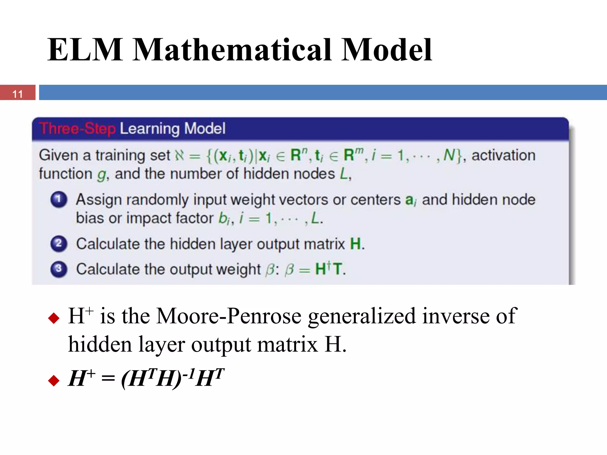
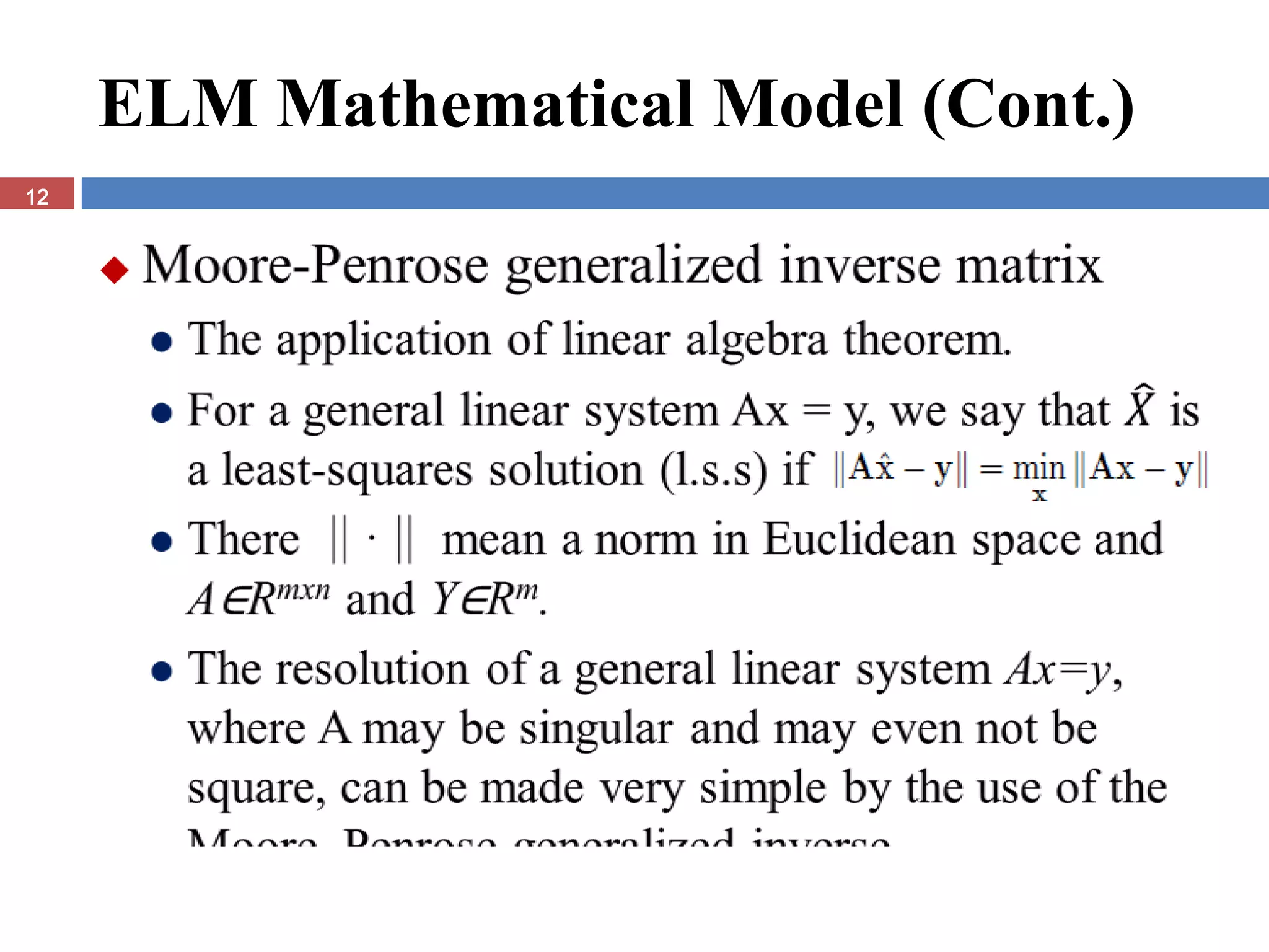
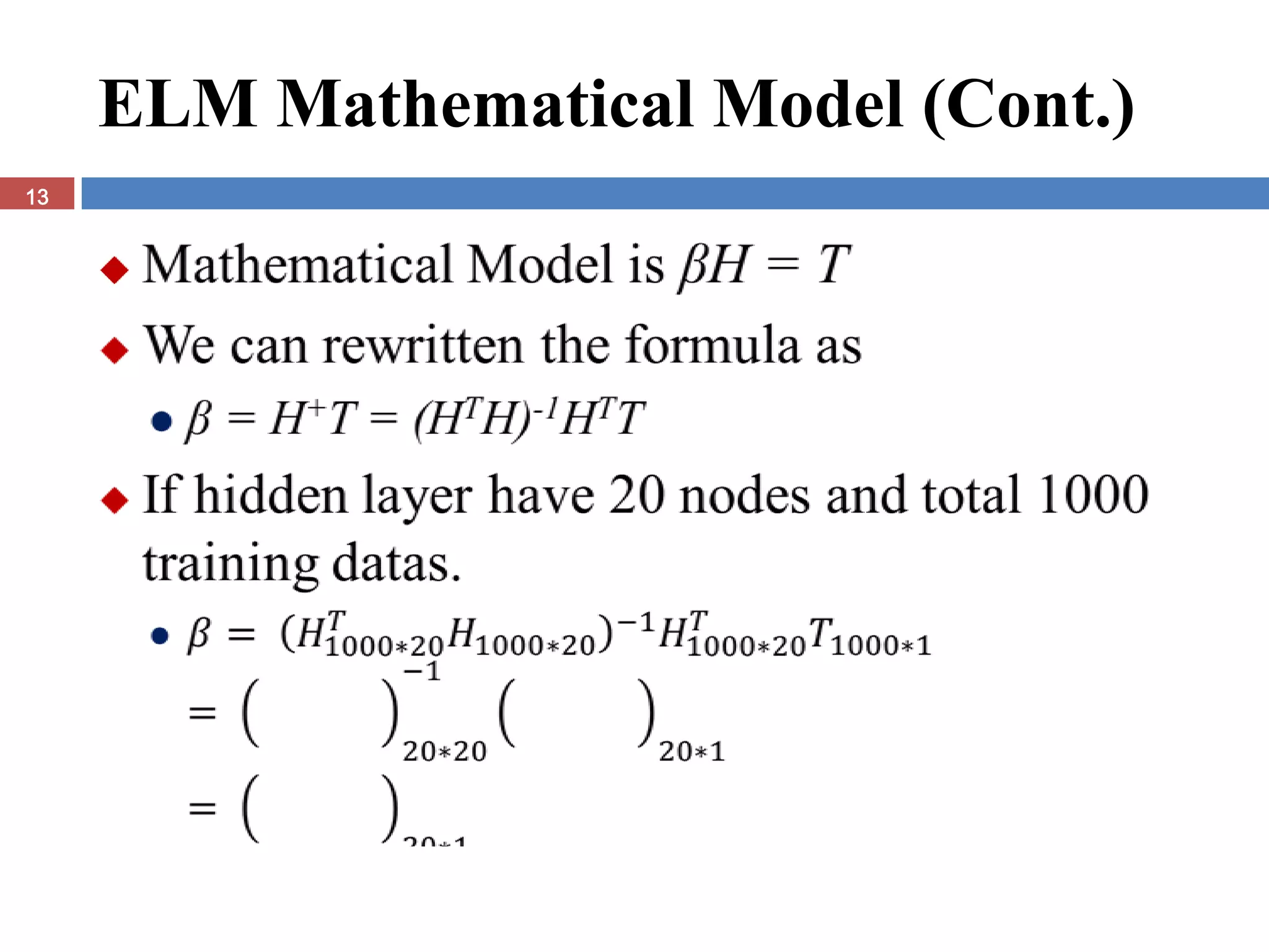
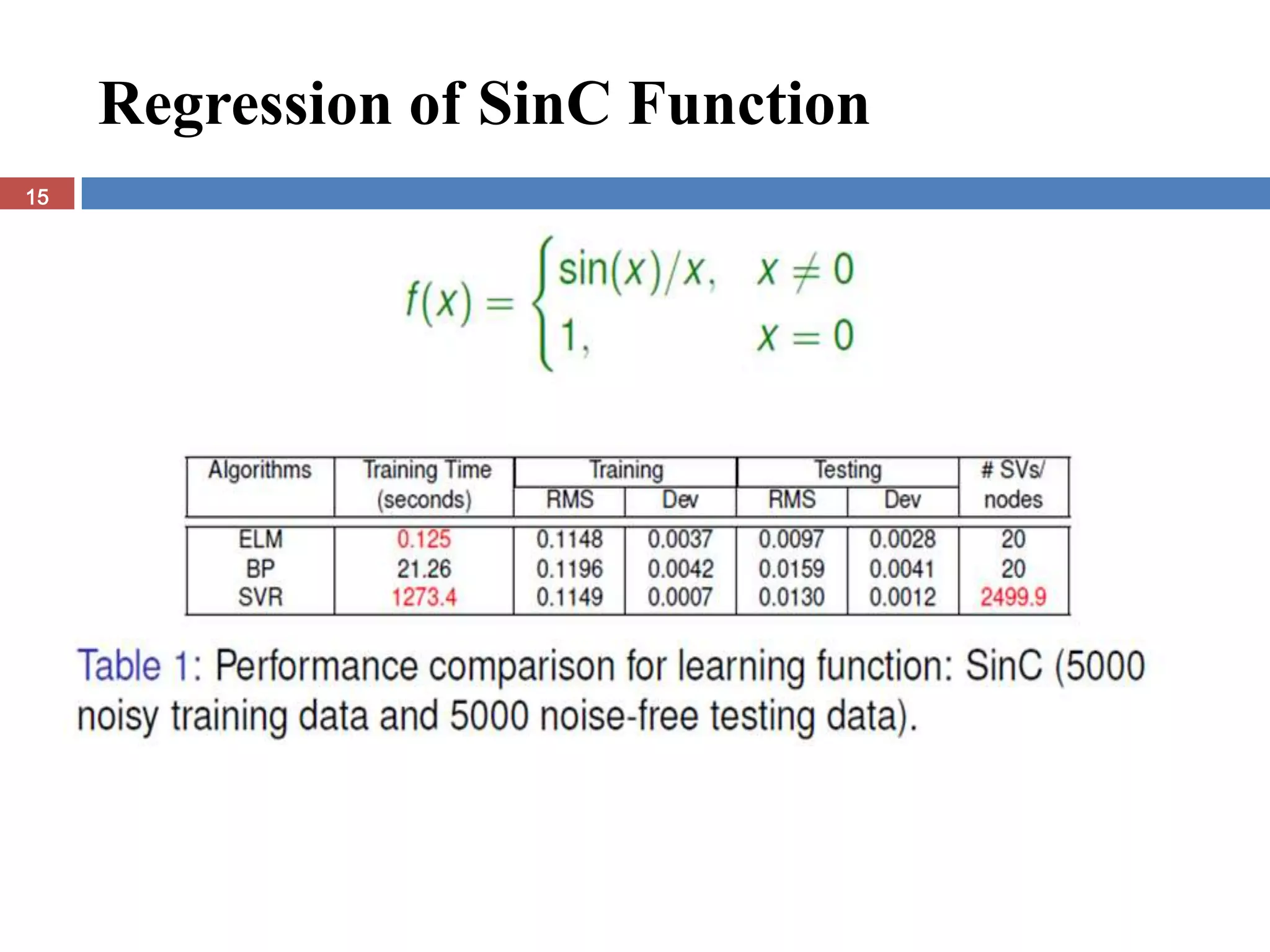
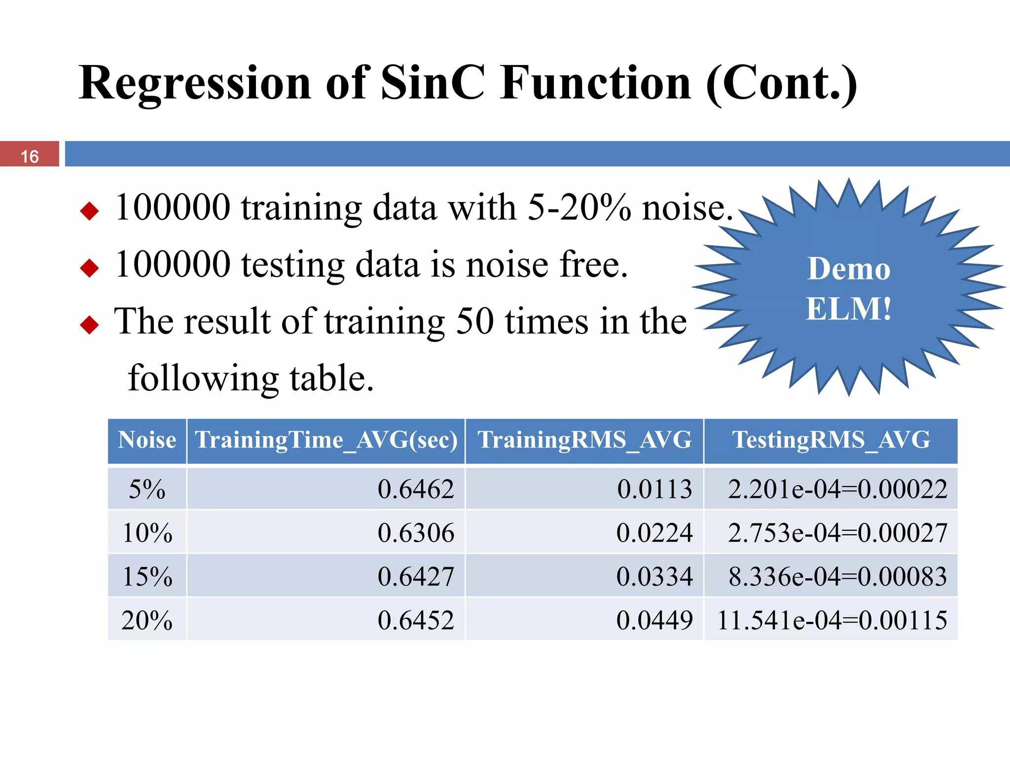
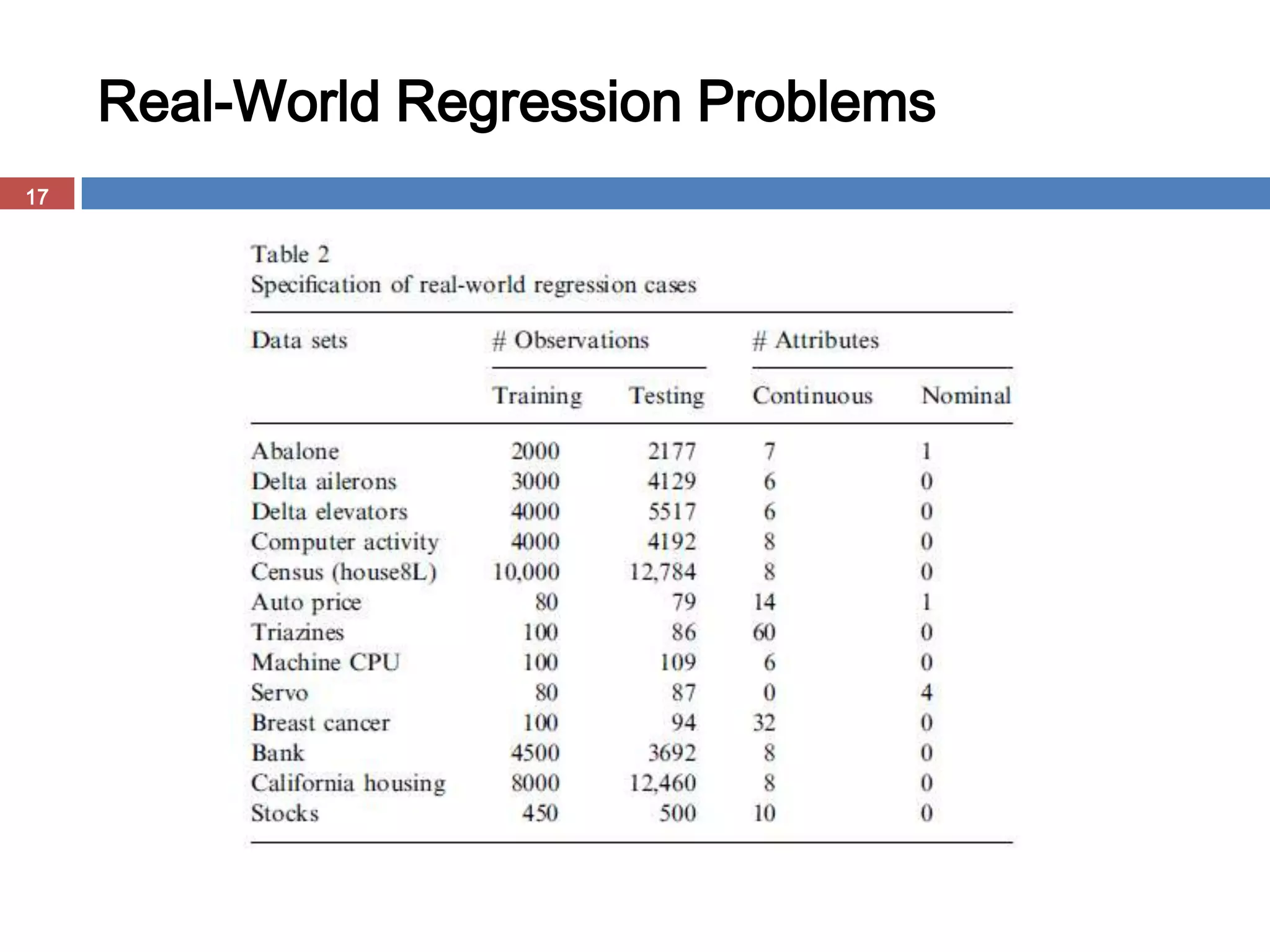
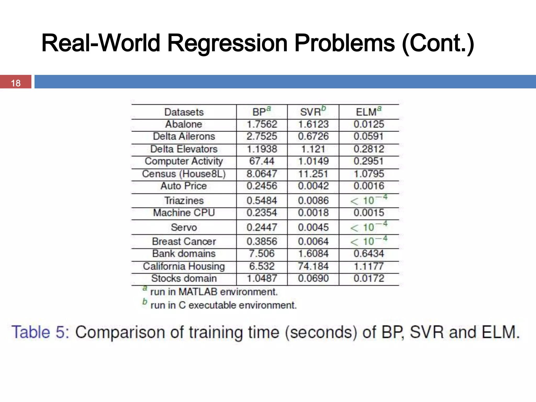
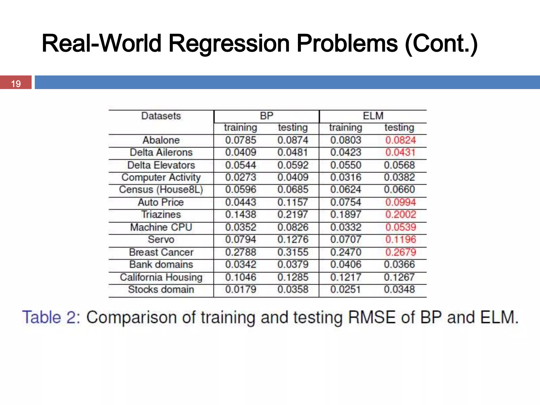
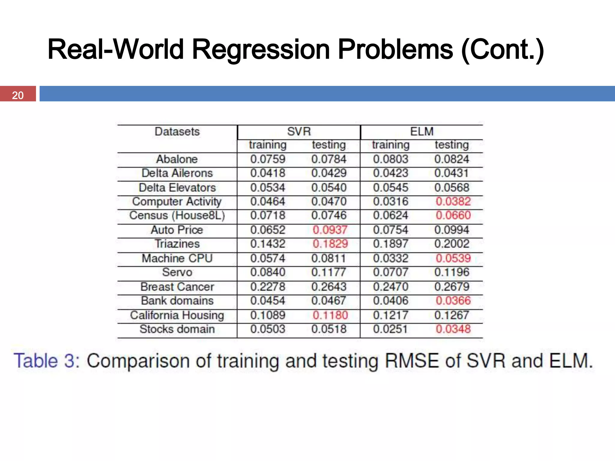
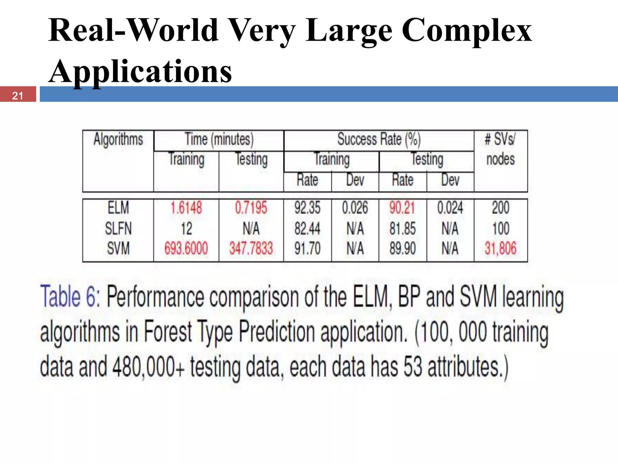
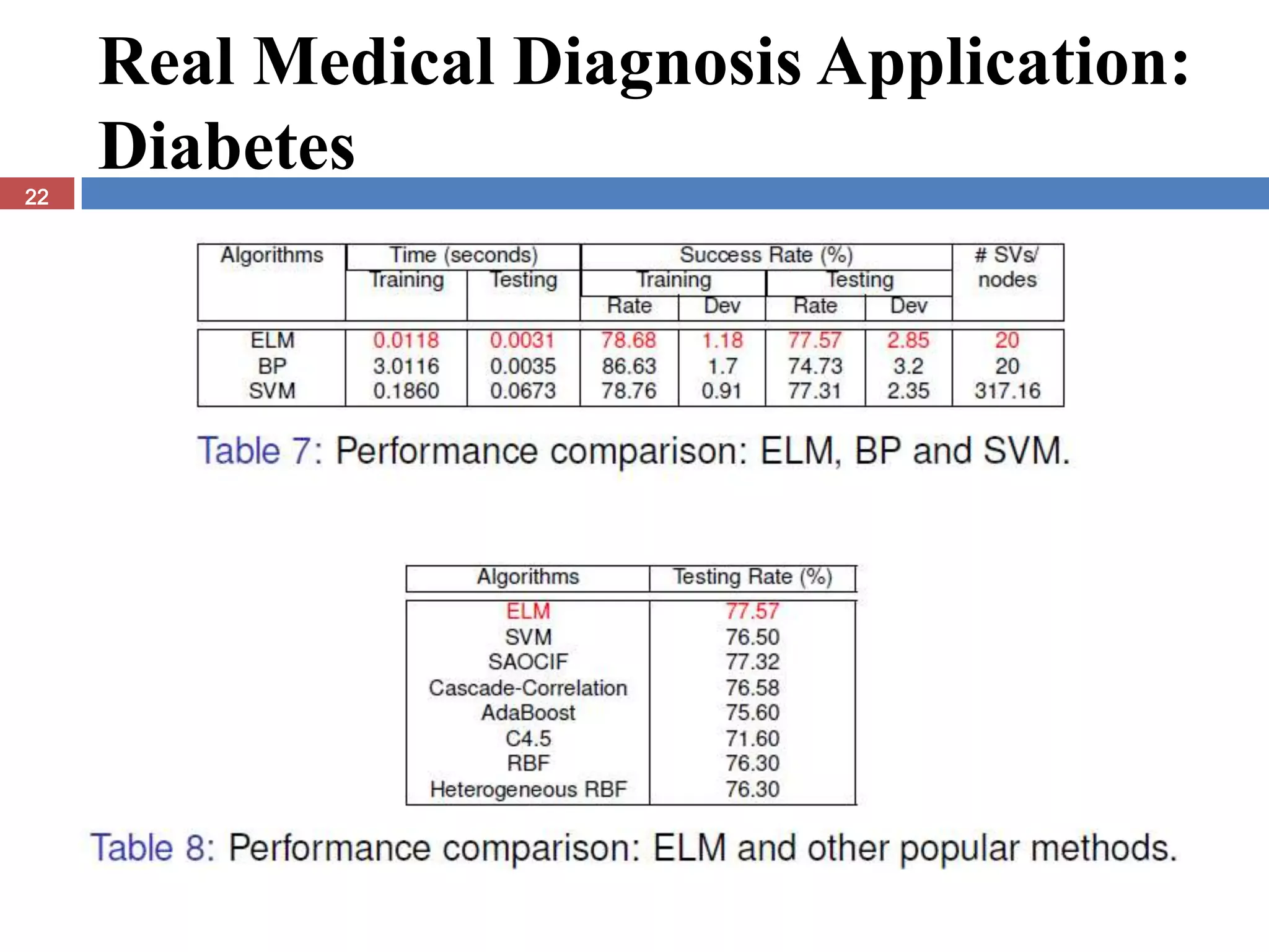
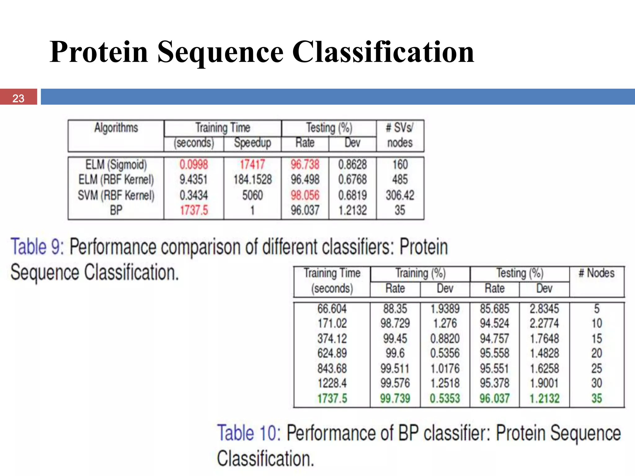
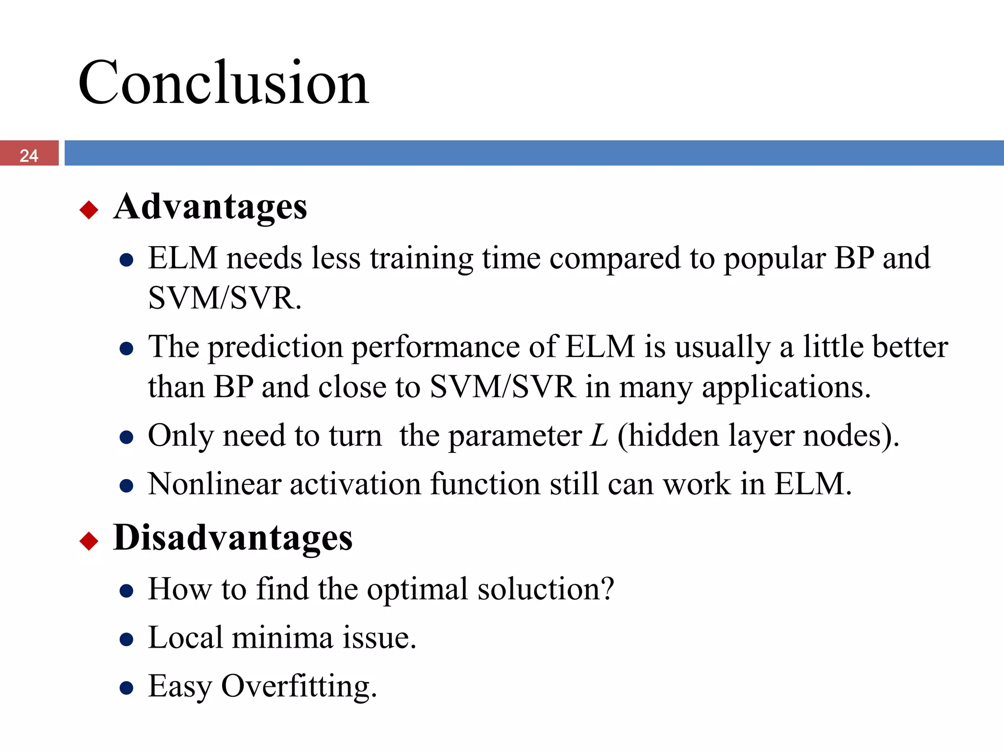
The document presents the extreme learning machine (ELM) theory and algorithm. ELM is a learning algorithm for single-hidden layer feedforward neural networks. Unlike traditional algorithms, ELM assigns input weights and hidden biases randomly and computes output weights through Moore-Penrose generalized inverse, making it faster than backpropagation. The paper evaluates ELM on regression and classification tasks, finding it achieves comparable or better performance than other algorithms while requiring less training time.

1. Extreme learning machine:Theory and applications
G.-B. Huang, Q.-Y. Zhu, and C.-K. Siew
Neurocomputing, 2006
Presenter: James Chou
2012/03/15

2. Outline
2
 Introduction
 Single-hidden layer feed-forward neural networks
 Neural Network Mathematical Model
 Back Propagation algorithm
 ELM Mathematical Model
 Performance Evaluation
 Conclusion

3. Introduction
3
 For past decades, gradient descent based methods have mainly
been used in many learning algorithms of feed-forward neural
networks.
 Traditionally, all the parameters of the feed-forward neural
networks need to tune iterative and need a very long time to
learn.
 When the input weights and the hidden layer biases are
randomly assigned, SLFNs (single-hidden layer feed-forward
neural networks) can be simply considered as a linear system
and the output weights (linking the hidden layer to the output
layer) can be computed through simple generalized inverse
operation.

4. Introduction (Cont.)
4
 Based on this idea, this paper proposes a simple learning
algorithm for SLFNs called extreme learning.
 Different from traditional learning algorithms the extreme
learning algorithm not only provide the smaller training
error but also the better performance.

5. Single-hidden layer feed-forward
5
neural networks
N
Output  F ( i xi   )
i 1
θ is the threshold
 F(．) is activation function
 Hard Limiter function

1, when x  
f ( x)  
0, when x  

 Sigmoid function
1
f ( x) 
1  e x

6. Single-hidden layer feed-forward
6
neural networks (Cont.)
G() is activation function
L is number of hidden layer nodes

7. Neural Network Mathematical Model
7

8. Neural Network Mathematical Model (Cont.)
8
If ε = 0 , mean
FL(x) = f(x) = T , T is known target
and
Cost function = 0

9. Neural Network Mathematical Model (Cont.)
9


10. Back Propagation algorithm
10
 BP algorithm is the classic gradient base algorithm to find the
best weight vectors and minimize the cost function.
Demo BP
algorithm!
η is Leaming Rate

11. ELM Mathematical Model
11
 H+ is the Moore-Penrose generalized inverse of
hidden layer output matrix H.
 H+ = (HTH)-1HT

12. ELM Mathematical Model (Cont.)
12


13. ELM Mathematical Model (Cont.)
13


15. Regression of SinC Function
15

16. Regression of SinC Function (Cont.)
16
 100000 training data with 5-20% noise.
 100000 testing data is noise free. Demo
 The result of training 50 times in the ELM!
following table.
Noise TrainingTime_AVG(sec) TrainingRMS_AVG TestingRMS_AVG
5% 0.6462 0.0113 2.201e-04=0.00022
10% 0.6306 0.0224 2.753e-04=0.00027
15% 0.6427 0.0334 8.336e-04=0.00083
20% 0.6452 0.0449 11.541e-04=0.00115

17. Real-World Regression Problems
17

18. Real-World Regression Problems (Cont.)
18

19. Real-World Regression Problems (Cont.)
19

20. Real-World Regression Problems (Cont.)
20

21. Real-World Very Large Complex
Applications
21

22. Real Medical Diagnosis Application:
Diabetes
22

23. Protein Sequence Classification
23

24. Conclusion
24
 Advantages
 ELM needs less training time compared to popular BP and
SVM/SVR.
 The prediction performance of ELM is usually a little better
than BP and close to SVM/SVR in many applications.
 Only need to turn the parameter L (hidden layer nodes).
 Nonlinear activation function still can work in ELM.
 Disadvantages
 How to find the optimal soluction?
 Local minima issue.
 Easy Overfitting.