1- Single Layer Perceptron ANN and Neural Networks
1.
CLO3: Artificial NeuralNetwork
Part 1: Single-layer Perceptron
ELE 4643: Intelligent Systems
2.
Artificial Neural Networks:
SupervisedLearning
Objectives
Introduction, or how the brain works
The neuron as a simple computing
element
The perceptron
3.
The Brain
• Ourbrain can be considered as a highly
complex, non-linear and parallel information-
processing system (neurons)..
• Information is stored and processed in a neural
network simultaneously throughout the whole
network, rather than at specific locations. In
other words, in neural networks, both data and
its processing are global rather than local
4.
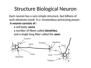
Structure Biological Neuron
Eachneuron has a very simple structure, but billions of
such elements result in a tremendous processing power..
A neuron consists of :
a cell body, soma
a number of fibers called dendrites,
and a single long fiber called the axon
5.
Learning Neural Network
•Learning is a fundamental and essential
characteristic of biological neural networks.. The
ease with which they can learn led to attempts
to emulate a biological neural network in a
computer..
6.
Artificial Neural Network
•An Artificial Neural Network (ANN) is a
computational model that is inspired by biological
neural networks in the human brain and how
information is processed. Artificial Neural
Networks have are the source of excitement in
artificial intelligence due to recent breakthroughs
in speech recognition, computer vision and text
processing.
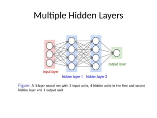
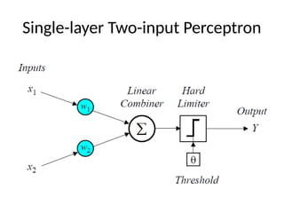
Single Neuron
The basicunit of computation in a neural network is the neuron,
sometimes called a node or unit. It receives input from nodes, or from
an external source and computes an output. Each input has an
associated weight (w), which is assigned based on the strength of
connection to the inputs. The node applies a function f (Activation
Function) to the weighted sum of its inputs and a bias as shown in the
Figure below:
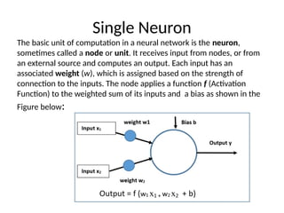
Operation of aNeuron
• The neuron takes numerical inputs X1 and X2 and the
associated weights w1 and w2 . Additionally, there is only
one Bias b associated each neuron.
• The output Y of each neuron is computed. The function f is
non-linear and is called the Activation Function. The purpose
of the activation function is to introduce non-linearity into
the output of a neuron. This is important because most real
world data is non linear.
• Every activation function takes the sum of weighted inputs
and the bias and performs a certain mathematical operation.
There are several activation functions to choose from
12.
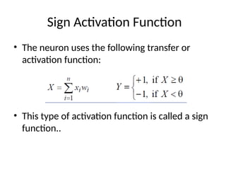
Sign Activation Function
•The neuron uses the following transfer or
activation function:
• This type of activation function is called a sign
function..
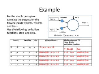
Example
Inputs Weights biasWeighed Inputs Find the Output Of
Step & Relu
Activation function
X1 X2 w1 w2 b Z = w1 x1 + w2 x2 + b
Y = Step(Z) Relu
0 0 1 1 -1.5 (0)(1) +(0)(1) – 1.5 = -1.5 Z < 0 , Y = 0 Max(0,-1.5) =0
0 1 1 1 -1.5 (0)(1) +(1)(1) – 1.5 = -0.5 Z < 0 , Y = 0 Max(0,-0.5) =0
1 0 1 1 -1.5 (1)(1) +(0)(1) – 1.5 = -0.5 Z < 0 , Y = 0 Max(0,-0.5) =0
1 1 1 1 -1.5 (1)(1) +(1)(1) – 1.5 = 0.5 Z < 0 , Y = 1 Max(0,0.5) =0.5
For the simple perceptron
calculate the outputs for the
flowing inputs weights, weights
and bias .
Use the following activation
functions: Step and Relu.
16.
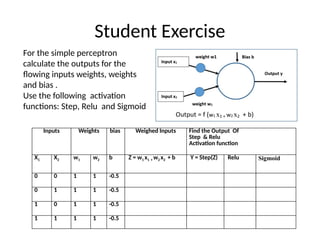
Student Exercise
Inputs Weightsbias Weighed Inputs Find the Output Of
Step & Relu
Activation function
X1 X2 w1 w2 b Z = w1 x1 + w2 x2 + b Y = Step(Z) Relu Sigmoid
0 0 1 1 -0.5
0 1 1 1 -0.5
1 0 1 1 -0.5
1 1 1 1 -0.5
For the simple perceptron
calculate the outputs for the
flowing inputs weights, weights
and bias .
Use the following activation
functions: Step, Relu and Sigmoid
17.
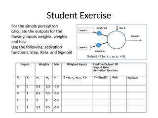
Student Exercise
Inputs Weightsbias Weighed Inputs Find the Output Of
Step & Relu
Activation function
X1 X2 w1 w2 b Z = w1 x1 + w2 x2 + b Y = Step(Z) Relu Sigmoid
0 0 0.3 0.2 -0.5
0 1 0.5 0.5 -0.5
1 0 1 0 -0.5
1 1 1.2 0.5 -0.5
For the simple perceptron
calculate the outputs for the
flowing inputs weights, weights
and bias .
Use the following activation
functions: Step, Relu and Sigmoid
Can a singleneuron learn a task?
The perceptron is the simplest form of
a neural network.. It consists of a
single neuron with adjustable synaptic
weights and a hard limiter.
The Perceptron
• Themodel consists of a linear combiner
followed by a hard limiter.
• The weighted sum of the inputs is applied to
the hard limiter, which produces an output
equal to +1 if its input is positive and 0 if it is
negative..
23.
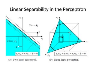
Pattern Classifier
• Theaim of the perceptron is to classify inputs,
x1, x2, . .., xn , into one of two classes, A1 and
A2.
• In the case of an elementary perceptron, the
dimensional space is divided by a hyper-plane
into two decision regions. The hyper-plane is
defined by the linearly separable function
How does theperceptron learn its
Classification tasks?
• This is done by making small adjustments in
the weights to reduce the difference between
the actual and desired outputs of the
perceptron. The initial weights are randomly
assigned, usually in the range [−0.5, 0.5], and
then updated to obtain the output consistent
with the training examples..
29.
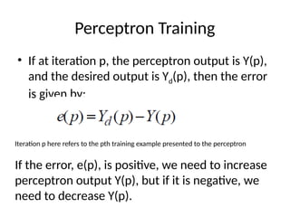
Perceptron Training
• Ifat iteration p, the perceptron output is Y(p),
and the desired output is Yd(p), then the error
is given by:
Iteration p here refers to the pth training example presented to the perceptron
If the error, e(p), is positive, we need to increase
perceptron output Y(p), but if it is negative, we
need to decrease Y(p).
30.
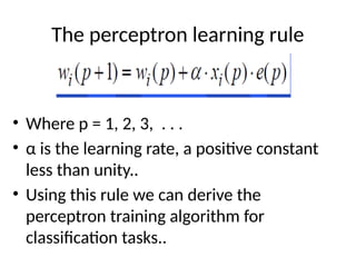
The perceptron learningrule
• Where p = 1, 2, 3, . . .
• α is the learning rate, a positive constant
less than unity..
• Using this rule we can derive the
perceptron training algorithm for
classification tasks..
31.
Perceptron’s training algorithm
31
Step1: Initialisation
Set initial weights w1, w2,…, wn and threshold
to random numbers in the range [0.5, 0.5].
Step 2: Activation
Activate the perceptron by applying inputs x1(p),
x2(p),…, xn(p) and desired output Yd (p).
Calculate the actual output at iteration p = 1
where n is the number of the perceptron inputs,
and step is a step activation function.
n
i
1
Y ( p ) step x i ( p ) wi
( p )
32.
Update the weightsof the perceptron
where wi(p) is the weight correction at iteration
p.
The weight correction is computed by the delta
rule:
Step 4: Iteration
Increase iteration p by one, go back to Step 2 and
repeat the process until convergence.
Perceptron’s training algorithm (continued)
Step 3: Weight training
22
wi ( p 1) wi ( p) wi ( p)
wi ( p) xi ( p)
e( p)
33.
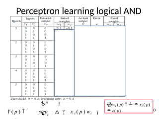
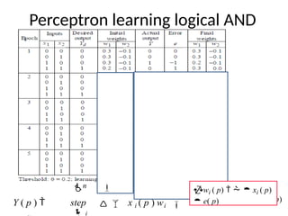
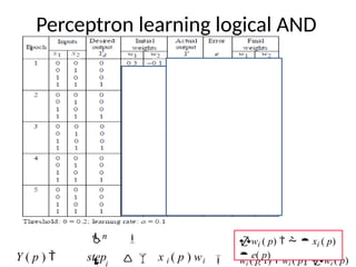
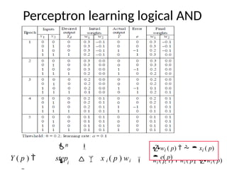
Perceptron learning logicalAND
wi ( p 1) wi ( p) wi ( p)
wi ( p) xi ( p)
e( p)
n
i
Y ( p ) step x i ( p ) wi
34.
Perceptron learning logicalAND
wi ( p 1) wi ( p) wi ( p)
wi ( p) xi ( p)
e( p)
n
i
Y ( p ) step x i ( p ) wi
35.
Perceptron learning logicalAND
wi ( p 1) wi ( p) wi ( p)
wi ( p) xi ( p)
e( p)
n
i
Y ( p ) step x i ( p ) wi
36.
Perceptron learning logicalAND
wi ( p 1) wi ( p) wi ( p)
wi ( p) xi ( p)
e( p)
n
i
Y ( p ) step x i ( p ) wi
37.
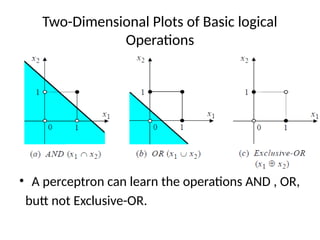
Two-Dimensional Plots ofBasic logical
Operations
• A perceptron can learn the operations AND , OR,
butt not Exclusive-OR.
38.
Decision Boundary
• Considerthe two-class classification task that consists of the following
points:
Class C1: [-1, -1], [-1, 1], [1, -1]
Class C2: [1, 1]
Which of the following equations can represent the decision boundary
between the two classes C1 and C2 using a single perceptron?
a) x1-x2-0.5=0
b) -x1+x2-0.5=0
c) 0.5(x1+x2)-1.5=0
d) x1+x2-0.5=0
39.
Decision Boundary
• Considerthe two-class classification task that consists of the following
points :
Class C1: [-1, -1], [-1, 1], [1, -1]
Class C2: [1, 1]
Which of the following equations can represent the decision boundary
between the two classes C1 and C2 using a single perceptron?
a) x1-x2-0.5=0
b) -x1+x2-0.5=0
c) 0.5(x1+x2)-1.5=0
d) x1+x2-0.5=0


![How does the perceptron learn its
Classification tasks?
• This is done by making small adjustments in
the weights to reduce the difference between
the actual and desired outputs of the
perceptron. The initial weights are randomly
assigned, usually in the range [−0.5, 0.5], and
then updated to obtain the output consistent
with the training examples..](https://image.slidesharecdn.com/1-singlelayerperceptronanns-250917170059-662700b4/85/1-Single-Layer-Perceptron-ANN-and-Neural-Networks-28-320.jpg)
![Perceptron’s training algorithm
31
Step 1: Initialisation
Set initial weights w1, w2,…, wn and threshold
to random numbers in the range [0.5, 0.5].
Step 2: Activation
Activate the perceptron by applying inputs x1(p),
x2(p),…, xn(p) and desired output Yd (p).
Calculate the actual output at iteration p = 1
where n is the number of the perceptron inputs,
and step is a step activation function.
n
i
1
Y ( p ) step x i ( p ) wi
( p ) ](https://image.slidesharecdn.com/1-singlelayerperceptronanns-250917170059-662700b4/85/1-Single-Layer-Perceptron-ANN-and-Neural-Networks-31-320.jpg)
![Decision Boundary
• Consider the two-class classification task that consists of the following
points:
Class C1: [-1, -1], [-1, 1], [1, -1]
Class C2: [1, 1]
Which of the following equations can represent the decision boundary
between the two classes C1 and C2 using a single perceptron?
a) x1-x2-0.5=0
b) -x1+x2-0.5=0
c) 0.5(x1+x2)-1.5=0
d) x1+x2-0.5=0](https://image.slidesharecdn.com/1-singlelayerperceptronanns-250917170059-662700b4/85/1-Single-Layer-Perceptron-ANN-and-Neural-Networks-38-320.jpg)
![Decision Boundary
• Consider the two-class classification task that consists of the following
points :
Class C1: [-1, -1], [-1, 1], [1, -1]
Class C2: [1, 1]
Which of the following equations can represent the decision boundary
between the two classes C1 and C2 using a single perceptron?
a) x1-x2-0.5=0
b) -x1+x2-0.5=0
c) 0.5(x1+x2)-1.5=0
d) x1+x2-0.5=0](https://image.slidesharecdn.com/1-singlelayerperceptronanns-250917170059-662700b4/85/1-Single-Layer-Perceptron-ANN-and-Neural-Networks-39-320.jpg)


![AI-Lecture-11[Neural Network] updated.pptx](https://cdn.slidesharecdn.com/ss_thumbnails/ai-lecture-11neuralnetworkupdated-251220065329-186ba89b-thumbnail.jpg?width=640&height=640&fit=bounds)