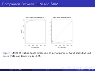
1. Comparison of Extreme Learning Machine with SVM
and Performance in Classification
Xiaoyu Sun
Department of Mathematics and Statistics
xysun@bu.edu
May 8, 2015
Xiaoyu Sun (BU) ELM May 8, 2015 1 / 21

2. Multiple Feed-forward Perceptrons Nerual Networks
Figure: A simple feed-forward perceptron with 8 input units, 2 layers of hidden
units, and 1 output unit. The gray-shading of the vector entries reflects their
numeric value. Cortes and Vapnik [1]
Xiaoyu Sun (BU) ELM May 8, 2015 2 / 21

3. Support Vector Networks
Figure: SVM can be considered as a specific type of single-hidden-layer
feed-forward network(SLFN). Cortes and Vapnik [1]
Xiaoyu Sun (BU) ELM May 8, 2015 3 / 21

4. BRIEF of SVMs
Suppose we have a training set {yi , xi }, i = 1, 2..., N, where yi
represents the class of the ith sample
Decision Function
f (x) = sign(
N
i=1
αi yi K(x, xi ) + b)
where K(x, xi ) is the ith hidden node in the last hidden layer of a
perception. αi yi is the output weight.
Optimization Problem
ˆf = argmin(
1
N
N
i=1
V (f (xi ), yi ) + λ f 2
)
Subject to: yi f (xi ) ≥ 1, i = 1, 2..., N
where λ is a user-specified parameter and provides a tradeoff between
training error and separating the margins.
Xiaoyu Sun (BU) ELM May 8, 2015 4 / 21

5. Soft Margins
Sometimes, we want to make sure we can always get a solution even in
high dimensional feature space, we need to consider the case that data
can’t be separated without errors.
Then we have
yi f (xi ) ≥ 1 − ξi , i = 1, 2..., N
ξi ≥ 0, i = 1, 2..., N
Xiaoyu Sun (BU) ELM May 8, 2015 5 / 21

6. More SVMs
We can choose different functions V and norm for training error and
smooth penalty. Therefore, there are some variants of SVM.
Here are two widely used examples.
1 Least Square Support Vector Machine (LS-SVM)
2 Proximal Support Vector Machine (PSVM)
Xiaoyu Sun (BU) ELM May 8, 2015 6 / 21

7. LS-SVM
In LS-SVM,
Minimize: LLS−SVM = 1
2 w 2 + λ1
2
N
i=1 ξ2
i
Subject to: yi (wφ(xi ) + b) = 1 − ξi , i = 1, 2..., N
Here, equality constraints are used, a set of linear equations instead of
quadratic constraints.
LS-SVM is proven to behave well generally and has lower
computational cost in many applications.
The decision function is the same as the conventional SVM.
f (x) = sign(
N
i=1
αi yi K(x, xi ) + b)
Where the Lagrange multipliers αi are proportional to the training
error ξi , while in the conventional SVM, many αi are typically equal
to zero.
Xiaoyu Sun (BU) ELM May 8, 2015 7 / 21

8. ELM
Suppose training set is {xi , yi };
A standard SLFN with L hidden neurons and activation function g(x) are
mathematically modeled as
L
i=1
βi g(wi xj + bi ) = oj , j = 1, 2..., N (∗)
where wi is the weight connecting the ith hidden neuron and the input
neurons. wi xj denotes the inner product.
βi is the weight connecting the ith hedden neuron and the output neurons.
Xiaoyu Sun (BU) ELM May 8, 2015 8 / 21

9. Support Vector Networks
Xiaoyu Sun (BU) ELM May 8, 2015 9 / 21

10. ELM
(∗) can be written in matrix form.
Hβ = Y
where the hidden-layer output matrix, H(w, x)
=



g(w1, x1 + b1) . . . g(wL, x1 + bL)
...
...
...
g(w1, xN + b1) . . . g(wL, xN + bL)



Xiaoyu Sun (BU) ELM May 8, 2015 10 / 21

11. ELM
Optimization Problem
We need to find ˆw, ˆb, ˆβ, such that,
Minimize: Hβ − Y and β
where Hβ − Y is the training error,
and the distance of margins of the two classes in the feature space is: 2
β
Xiaoyu Sun (BU) ELM May 8, 2015 11 / 21

12. Theorem
Moore-Penrose generalized inverse of matrix
A matrix G is the Moore-Penrose generalized inverse of matrix A, denoted
as A† , if
AGA = A, GAG = G, (AG)T
= AG, (GA)T
= GA
Theorem
Let there exist a matrix G such that Gy is a minimum norm least-square
solution of a linear system Ax = y as well as
Gy = arg min
x
Ax − y
Then it’s necessary and sufficient that G = A†, the Moore-Penrose
generalized inverse of matrix
Xiaoyu Sun (BU) ELM May 8, 2015 12 / 21

13. ELM
Therefore, there exists a unique solution of Hβ = Y
β = H†
Y (∗∗)
Algorithm ELM: Given a training set and an activation function g(x), and
hidden neuron number L.
Step 1: Assign arbitrary input weight wi and bias bi , i=1,2...,N.
Step 2: Calculate the hidden layer output matrix H.
Step 3: Calculate the output weight β using (**).
Xiaoyu Sun (BU) ELM May 8, 2015 13 / 21

14. Comparison Between ELM and SVM
Figure: Effect of sample size on performance of SVM and ELM, red line is SVM
and black line is ELM.
Xiaoyu Sun (BU) ELM May 8, 2015 14 / 21

15. Comparison Between ELM and SVM
Figure: Effect of feature space dimension on performance of SVM and ELM, red
line is SVM and black line is ELM.
Xiaoyu Sun (BU) ELM May 8, 2015 15 / 21

16. Comparison Between ELM and SVM
Number of Hidden Nodes Time Accuracy
10 9.560 0.8235294
100 8.164 0.8470588
1000 8.756 0.8529412
7129 18.904 0.8235294
Table: ELM with different number of nodes.
Xiaoyu Sun (BU) ELM May 8, 2015 16 / 21

17. Comparison Between ELM and SVM
Model Time Accuracy
SVM 55.400 0.8235294
LS-SVM 19.406 0.8529412
ELM 8.756 0.8529412
Table: Results of different model on cancer classification.
Xiaoyu Sun (BU) ELM May 8, 2015 17 / 21

18. Comparison Between ELM and SVM
Less Human Intervention than SVMs
In ELM, the hidden node parameter (w, b) are generated randomly,
and the performance is not very sensitive to the number of hidden
nodes L, although it has not been proved in theory yet, so the users
only need to specify the cost parameter C.
How does ELM behave with a wide range of number of hidden nodes
and what is the oscillation bound?
Xiaoyu Sun (BU) ELM May 8, 2015 18 / 21

19. Comparison Between ELM and SVM
Smaller Computational Complexity than SVMs with some dataset
It can be proved when the number of hidden nodes L is much smaller
than the number of training samples N, a.w.a, L N,ELM has
smaller computational cost than SVMs. However, what if N L,
high dimensions dataset such as cancer classification problem.
When comparing ELM and SVMs, we need to set the number of
hidden nodes L and the kernel the same, will ELM always has faster
speed or similar or even better generalization performance than
SVMs?
Xiaoyu Sun (BU) ELM May 8, 2015 19 / 21

20. Summary
In recent years, ELM has been proved can be applied in regression or
multiclass classification problems
ELM can do learning without iterative tuning which leads to less
human intervention and faster speed. It may be possible to
implement the online sequential variants of the kernel based ELM.
Many discussion about performance of ELM is based on data,
theoretical proof is still needed.
Xiaoyu Sun (BU) ELM May 8, 2015 20 / 21

21. Thank You
Xiaoyu Sun (BU) ELM May 8, 2015 21 / 21