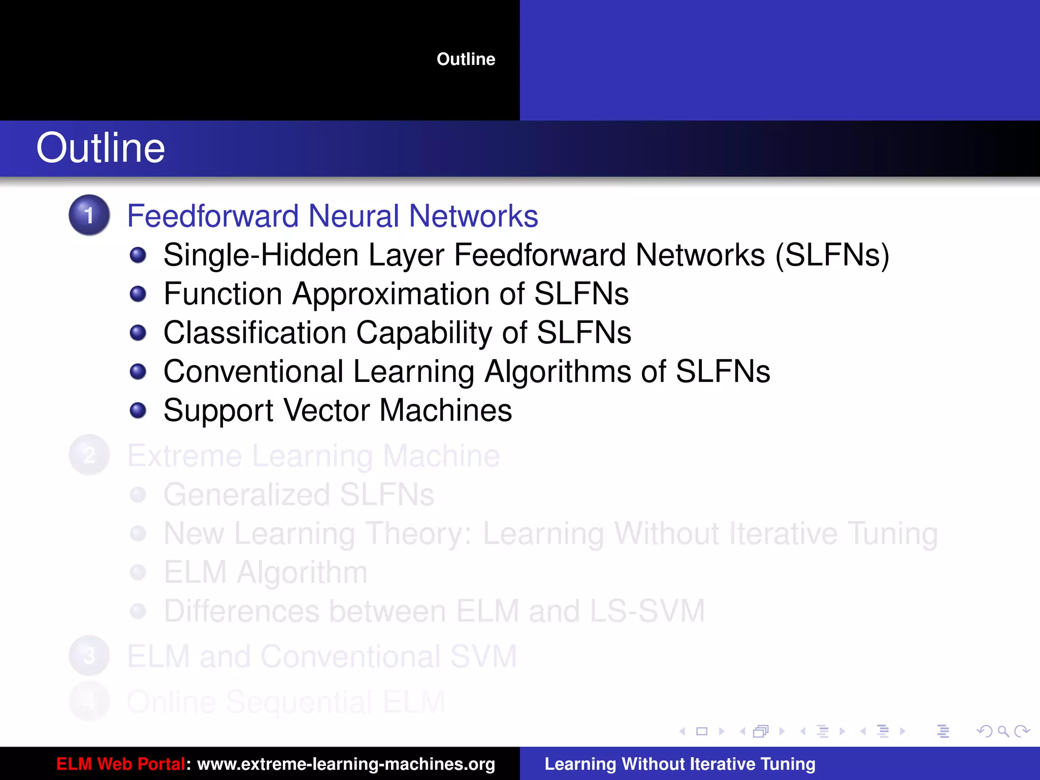
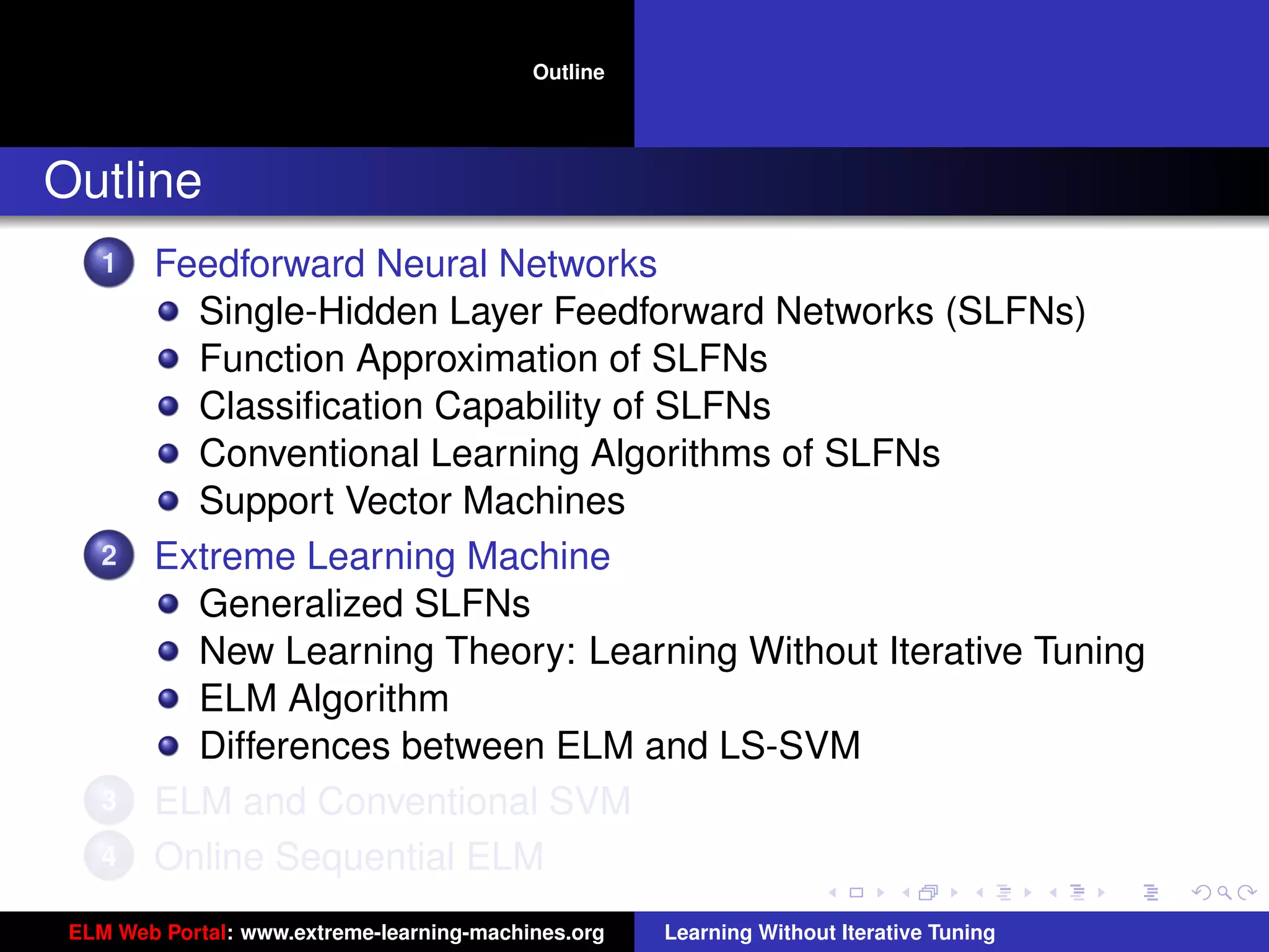
The document outlines a presentation on extreme learning machines (ELM). It includes four sections that cover: 1) feedforward neural networks and single-hidden layer feedforward networks (SLFNs), 2) ELM methodology including generalized SLFNs and learning without iterative tuning, 3) comparisons between ELM and conventional support vector machines (SVMs), and 4) online sequential ELM. The outline provides sub-topics to be discussed within each section.


![Feedforward Neural Networks
Generalized SLFNs
ELM
ELM Learning Theory
ELM and SVM
ELM Algorithm
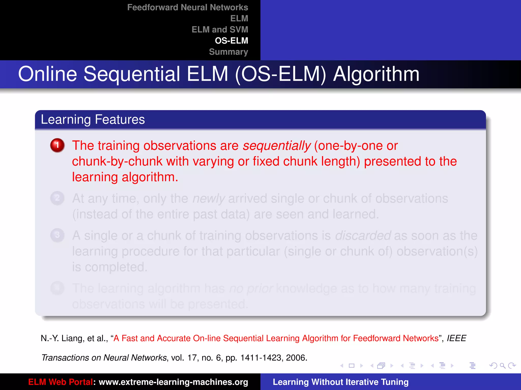
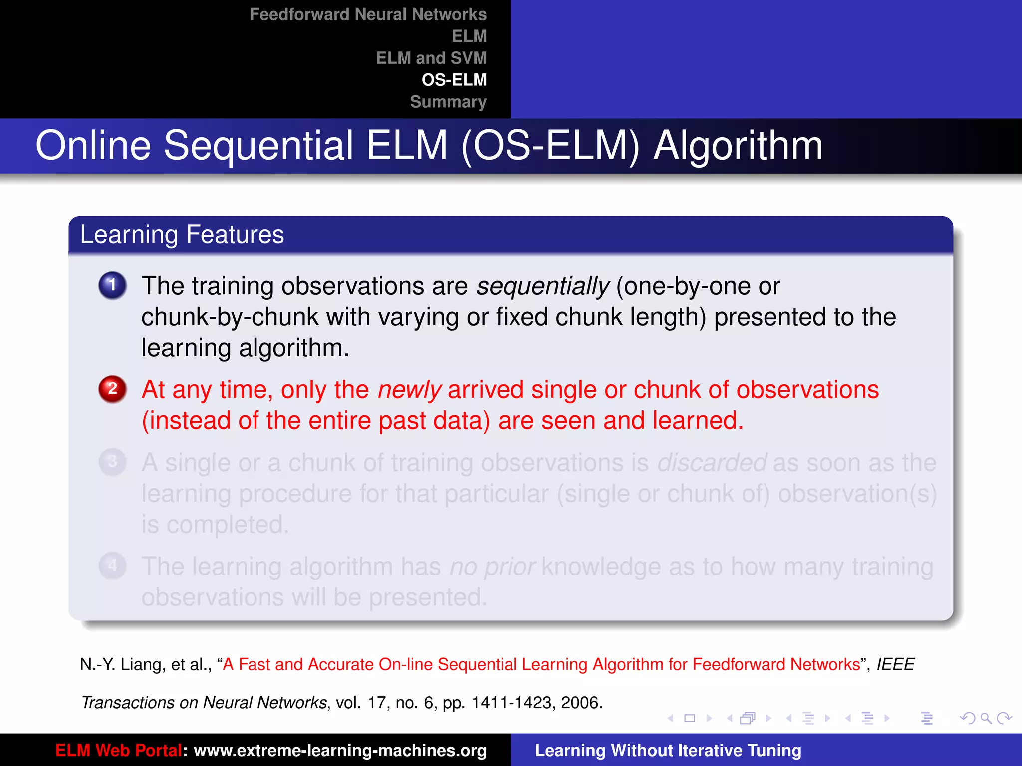
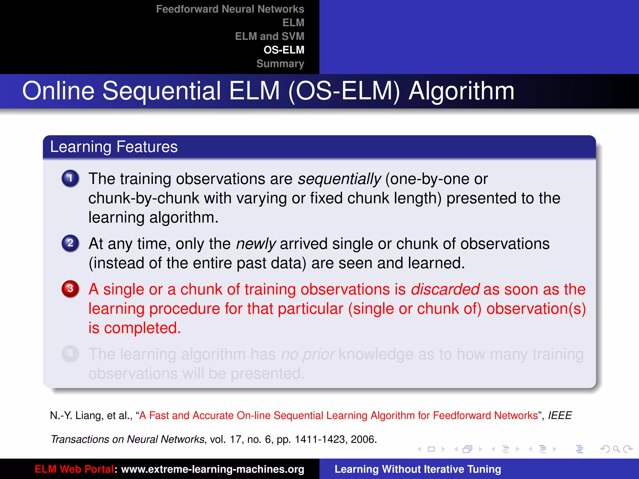
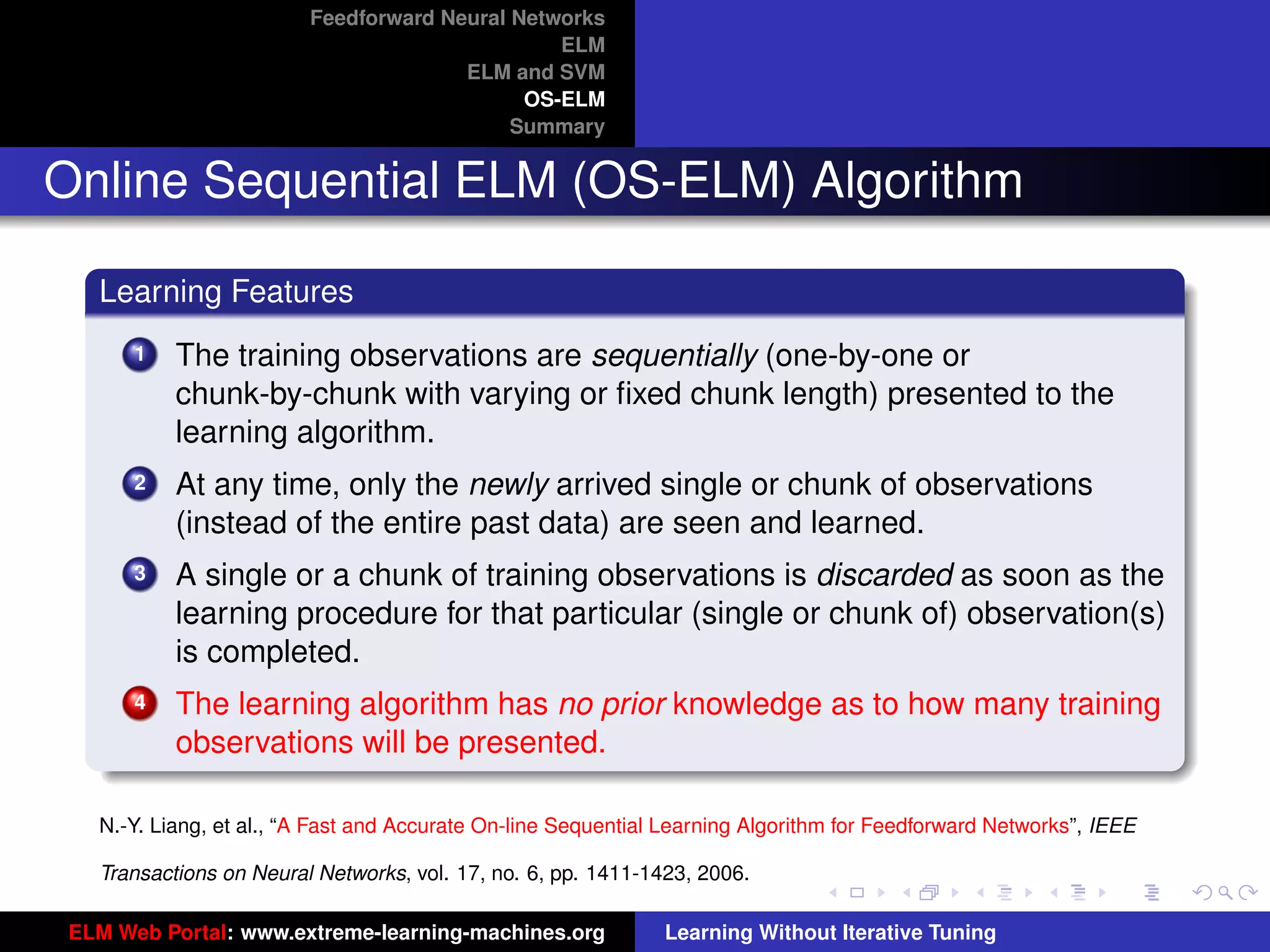
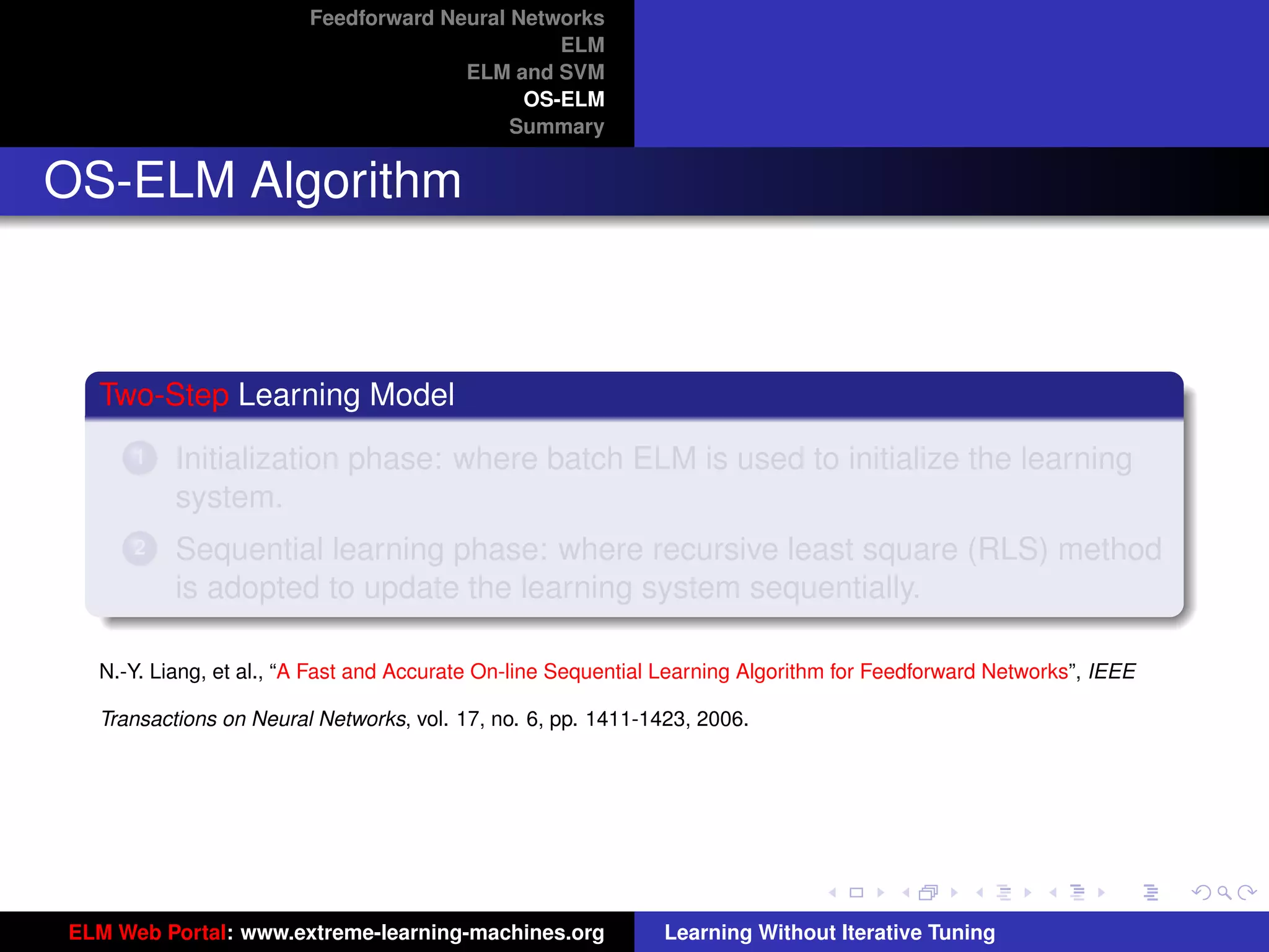
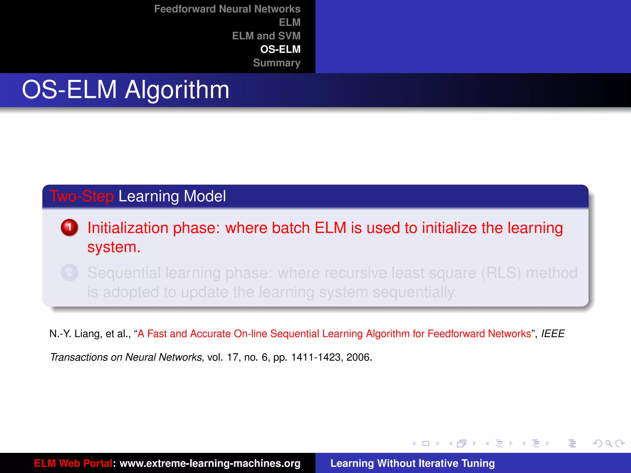
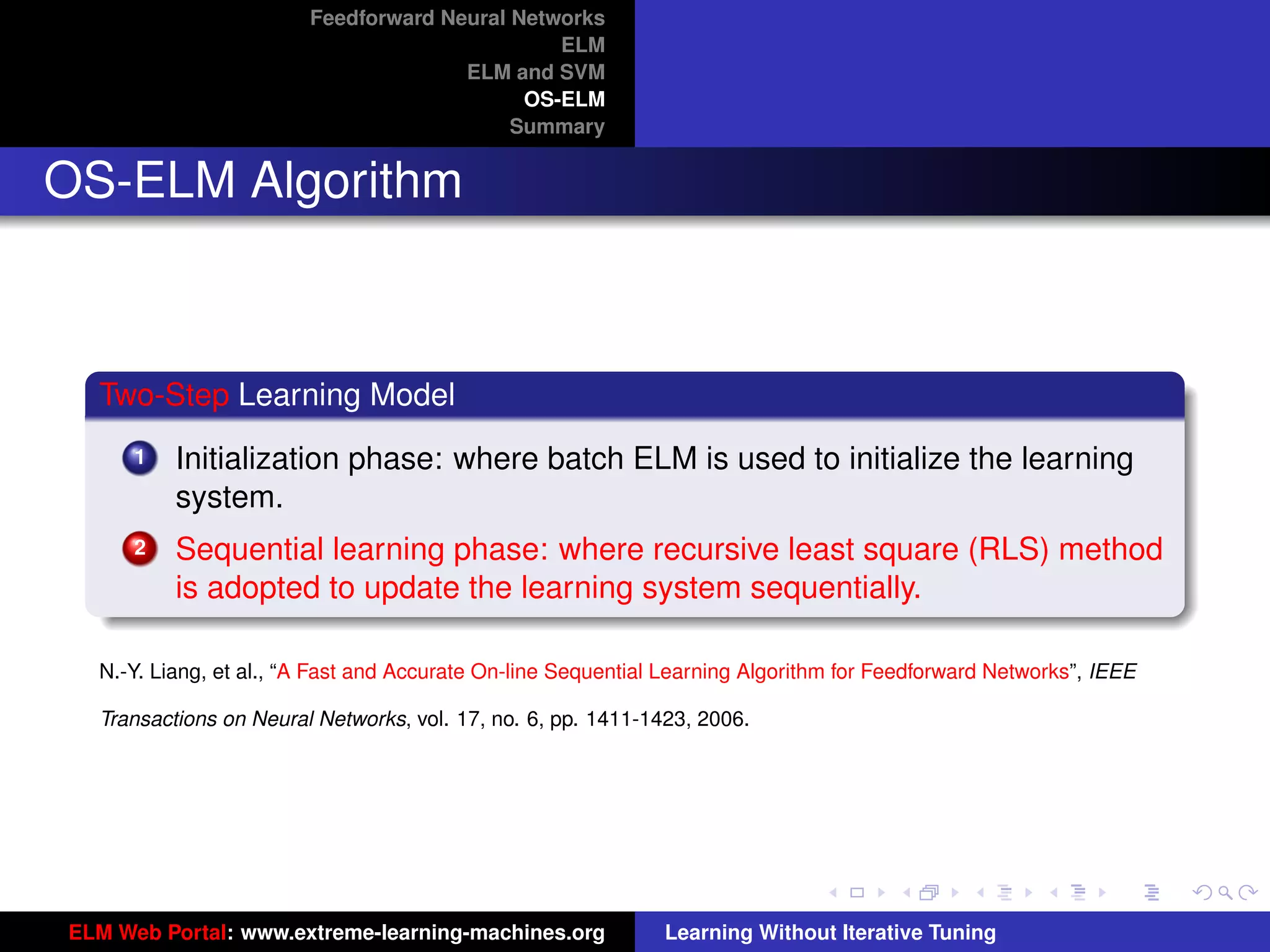
OS-ELM
ELM and LS-SVM
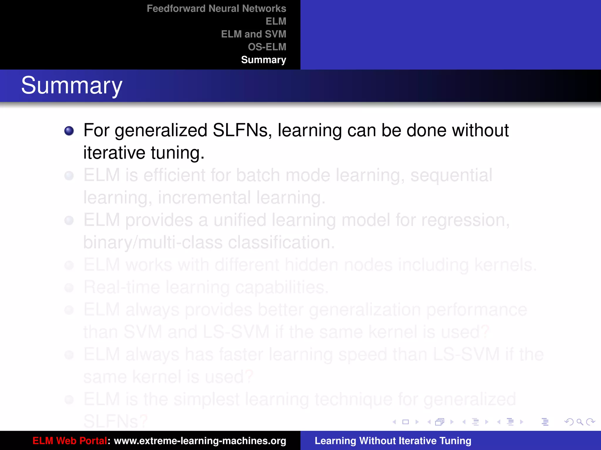
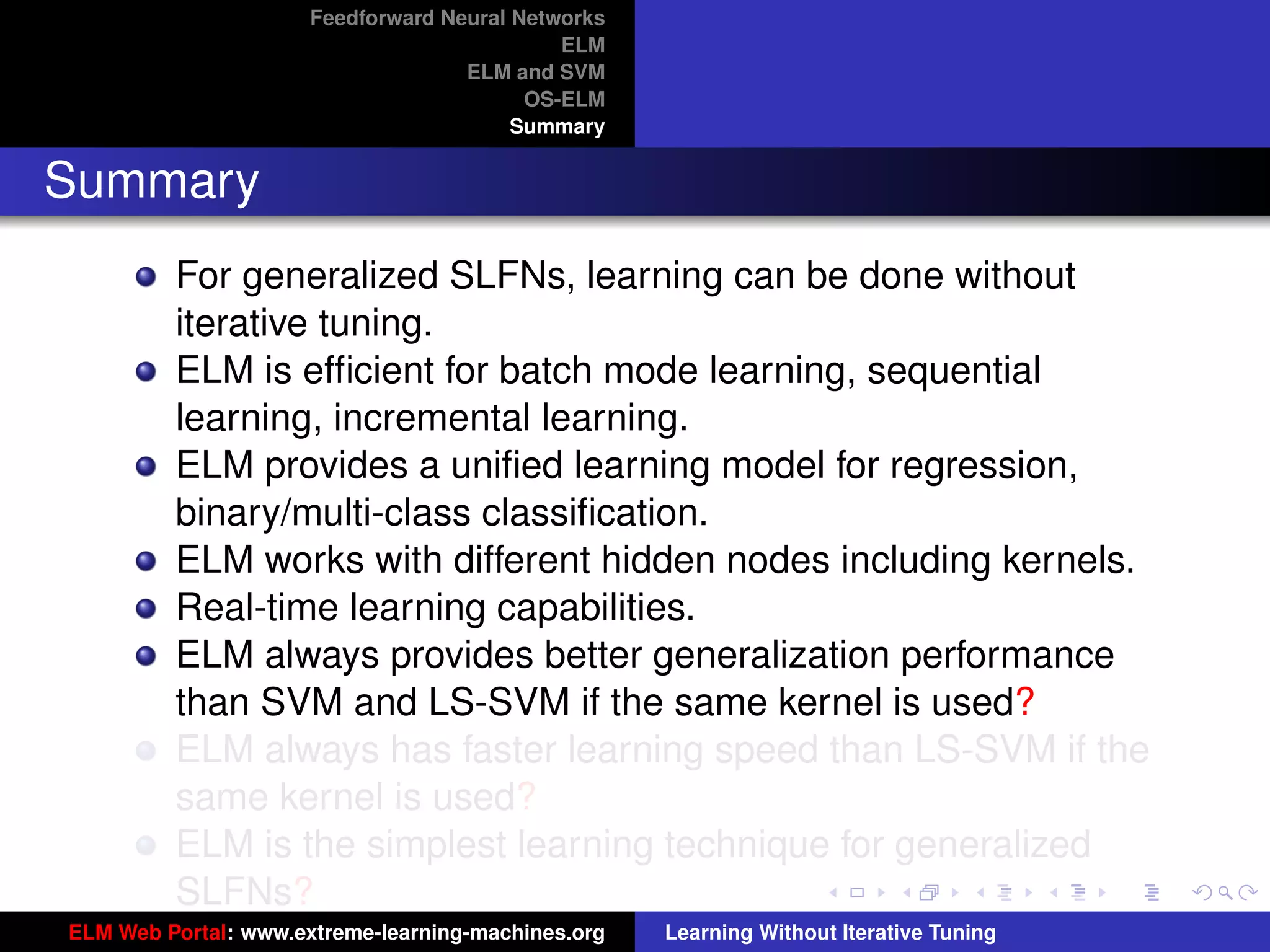
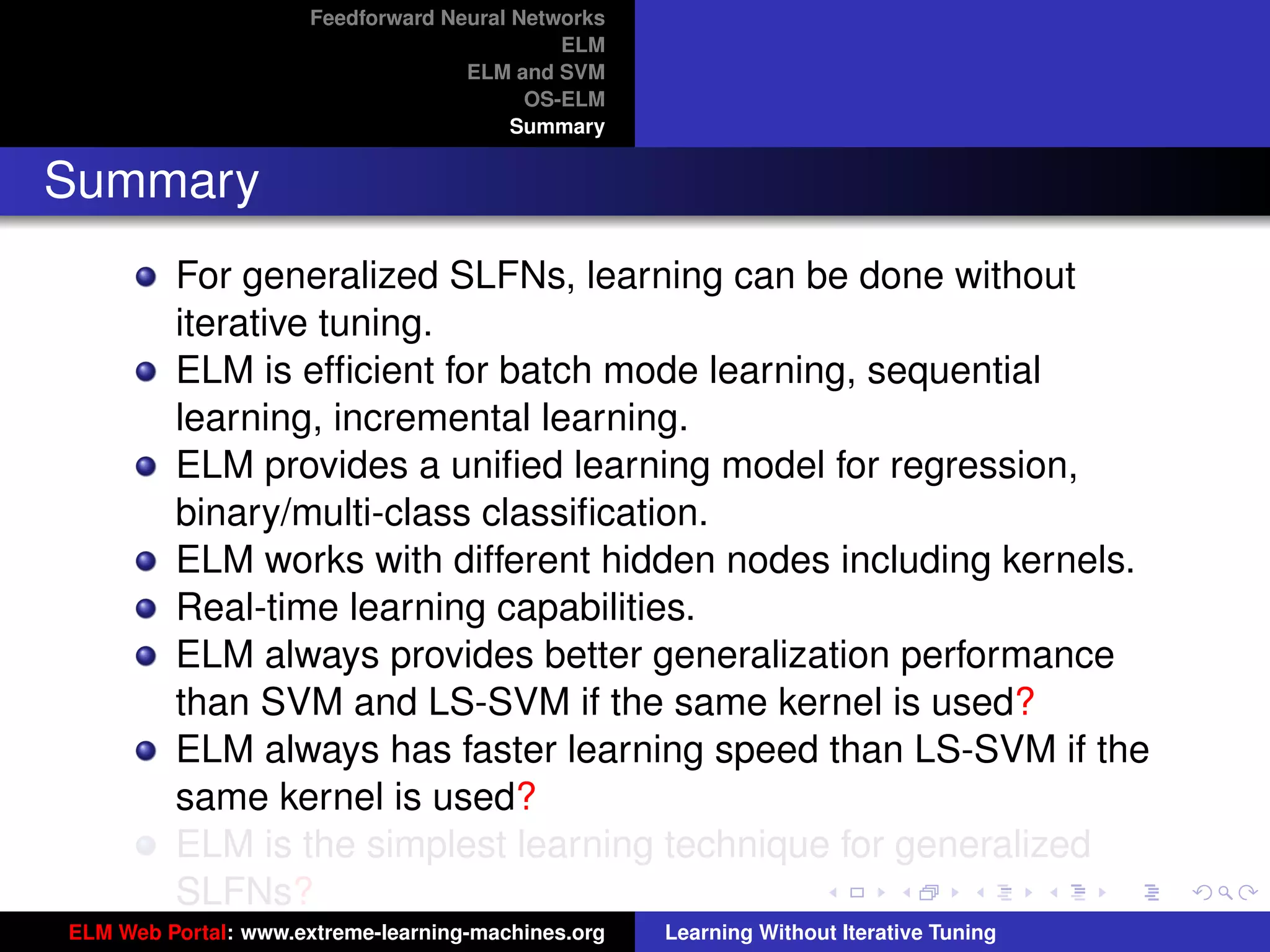
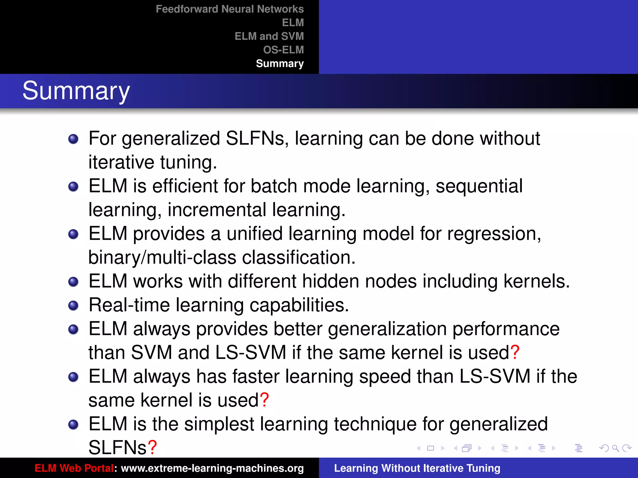
Summary
Generalized SLFNs
General Hidden Layer Mapping
PL
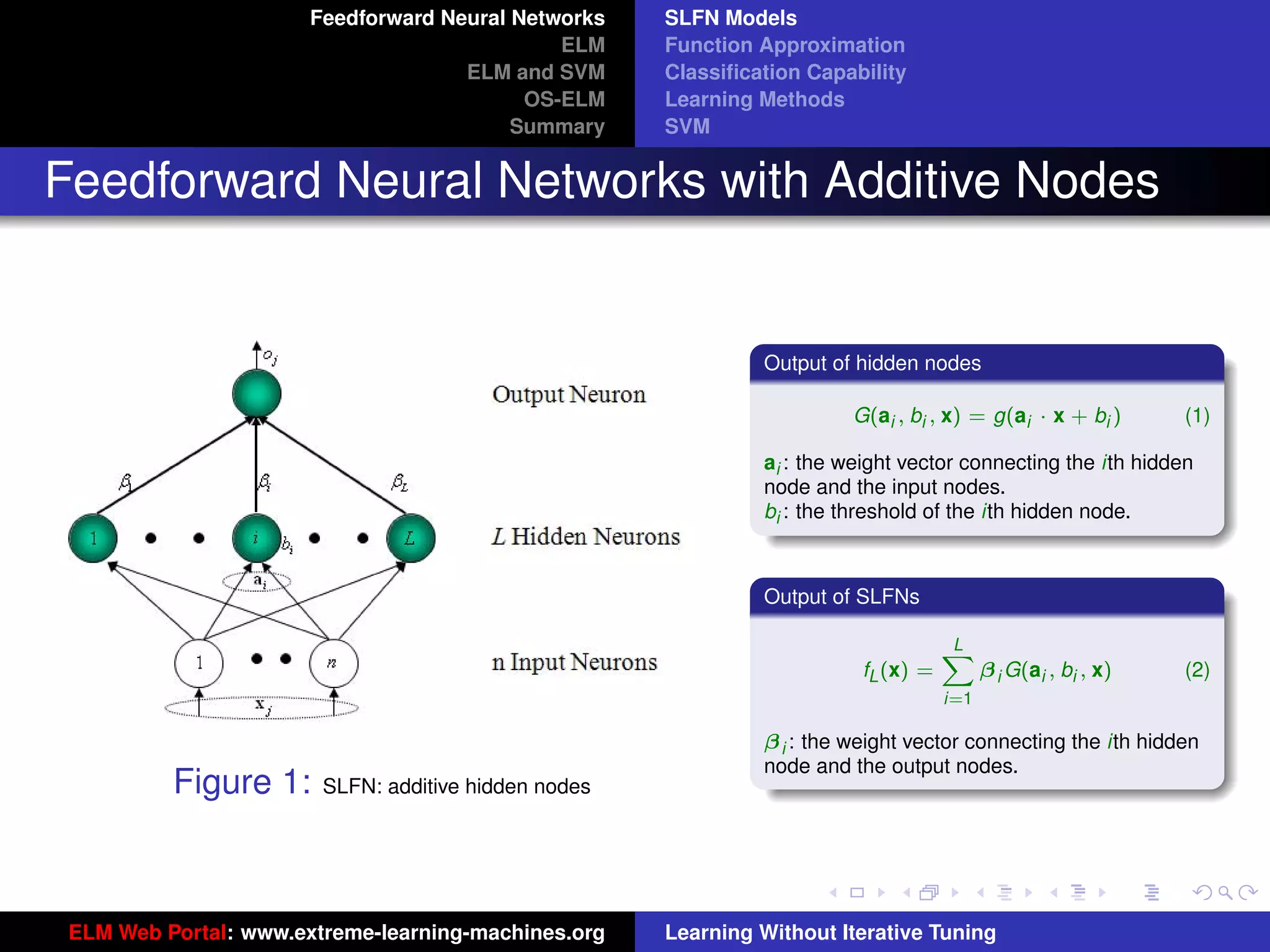
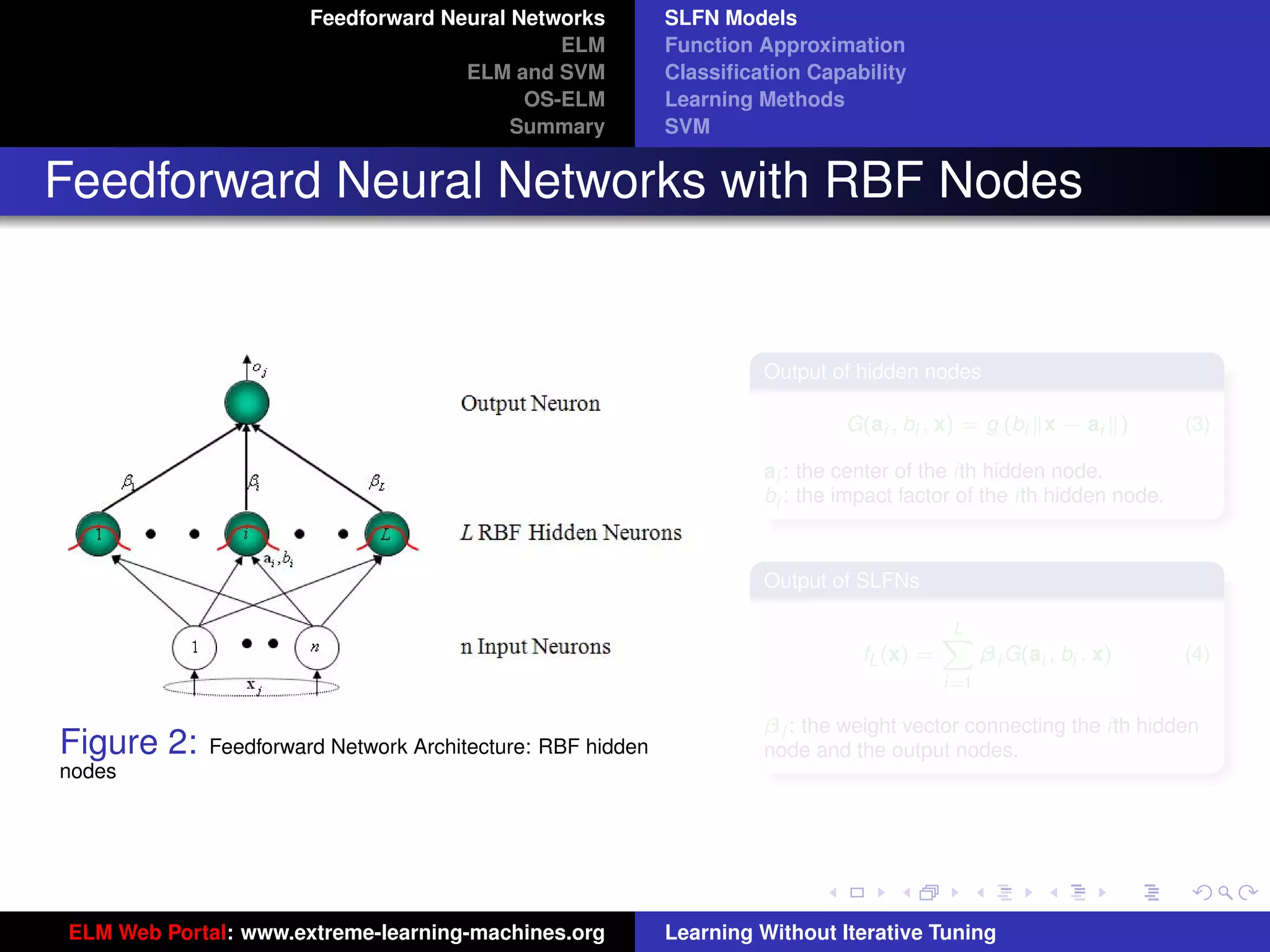
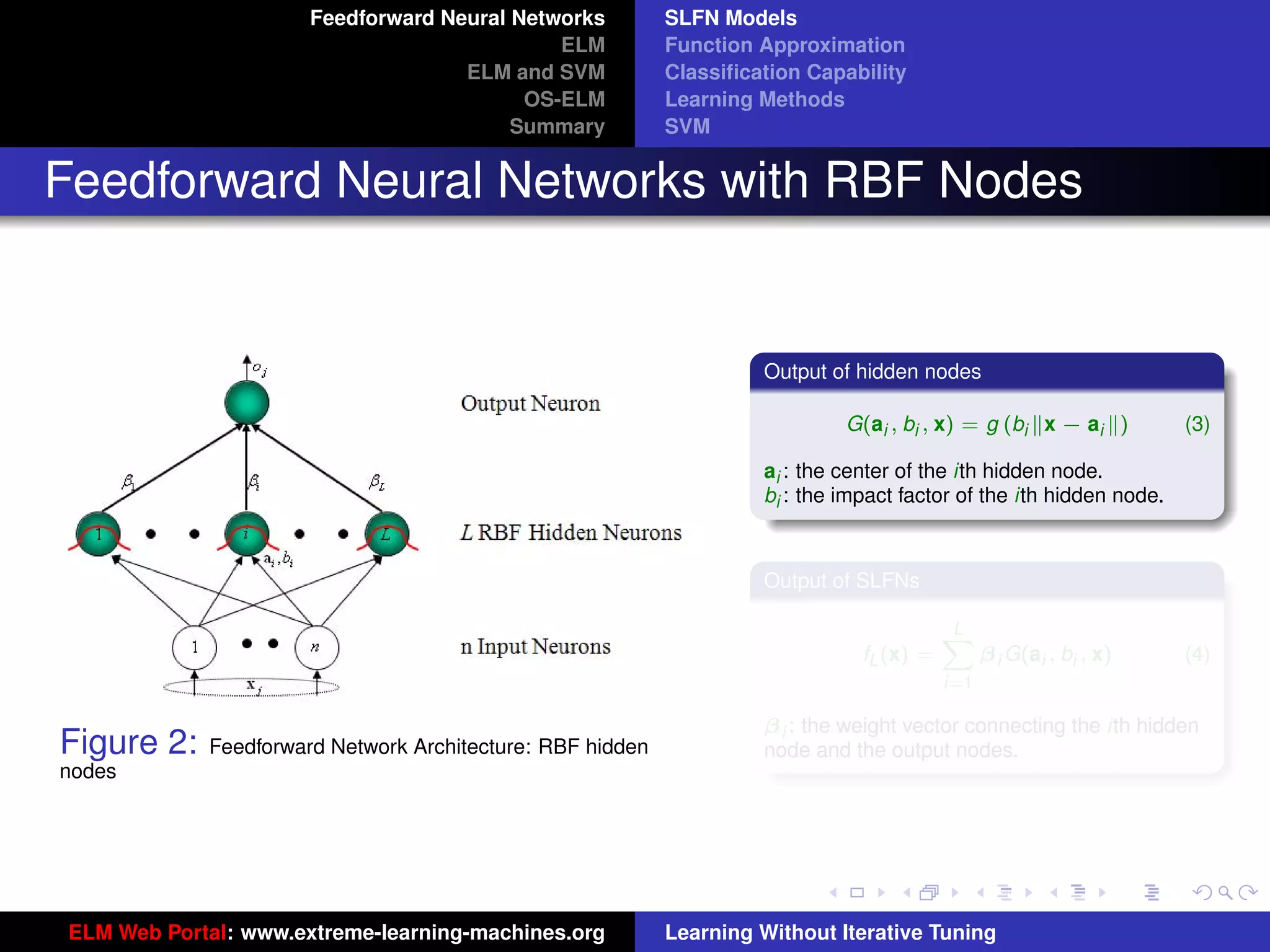
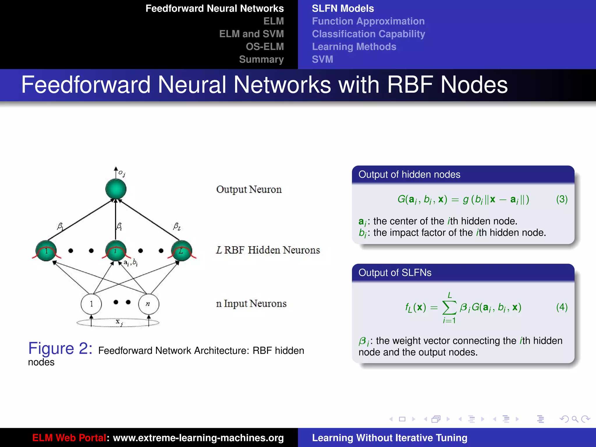
Output function: f (x) = i=1 β i G(ai , bi , x)
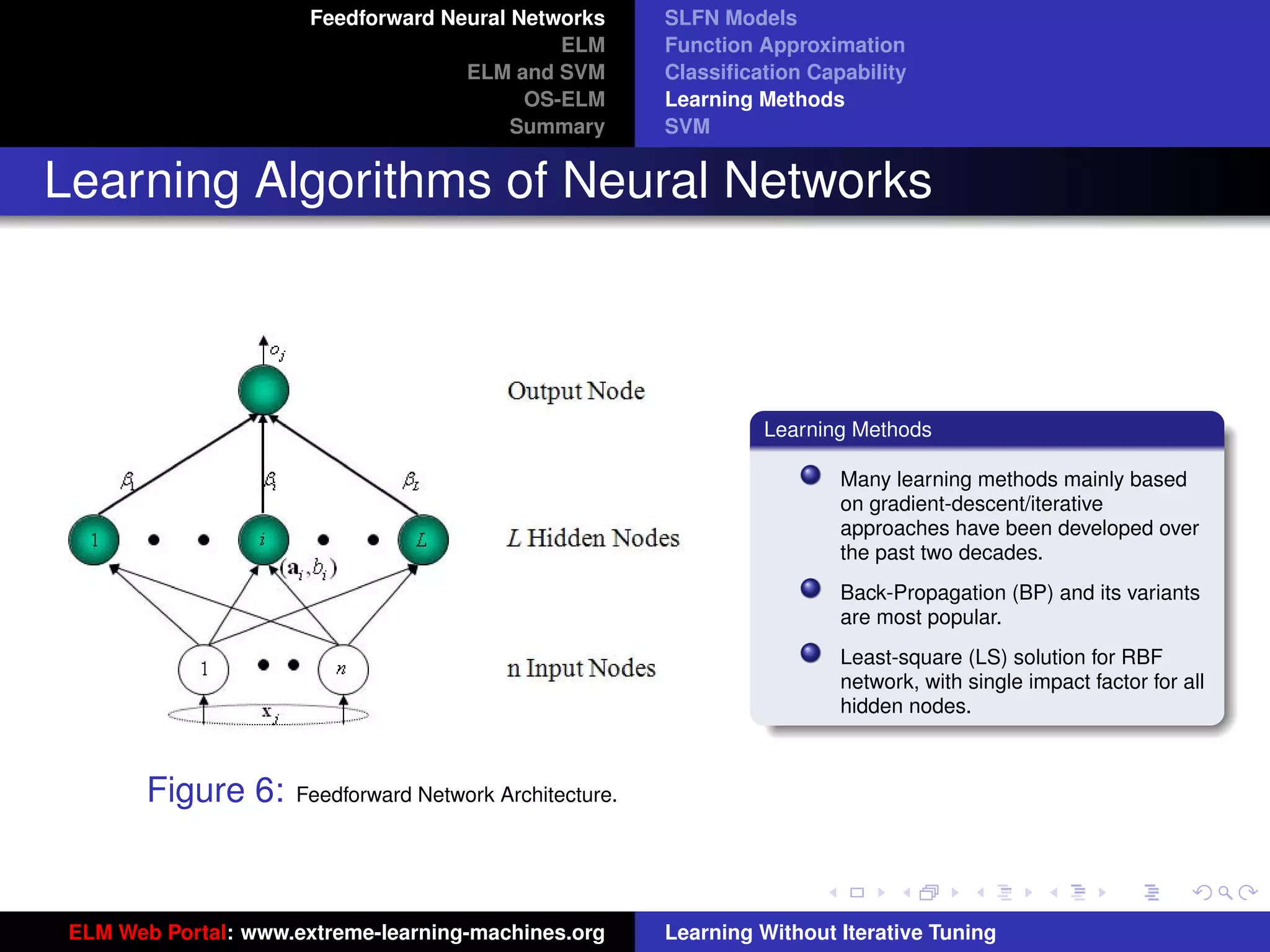
The hidden layer output function (hidden layer
mapping):
h(x) = [G(a1 , b1 , x), · · · , G(aL , bL , x)]
The output function needn’t be:
Sigmoid: G(ai , bi , x) = g(ai · x + bi )
RBF: G(ai , bi , x) = g (bi x − ai )
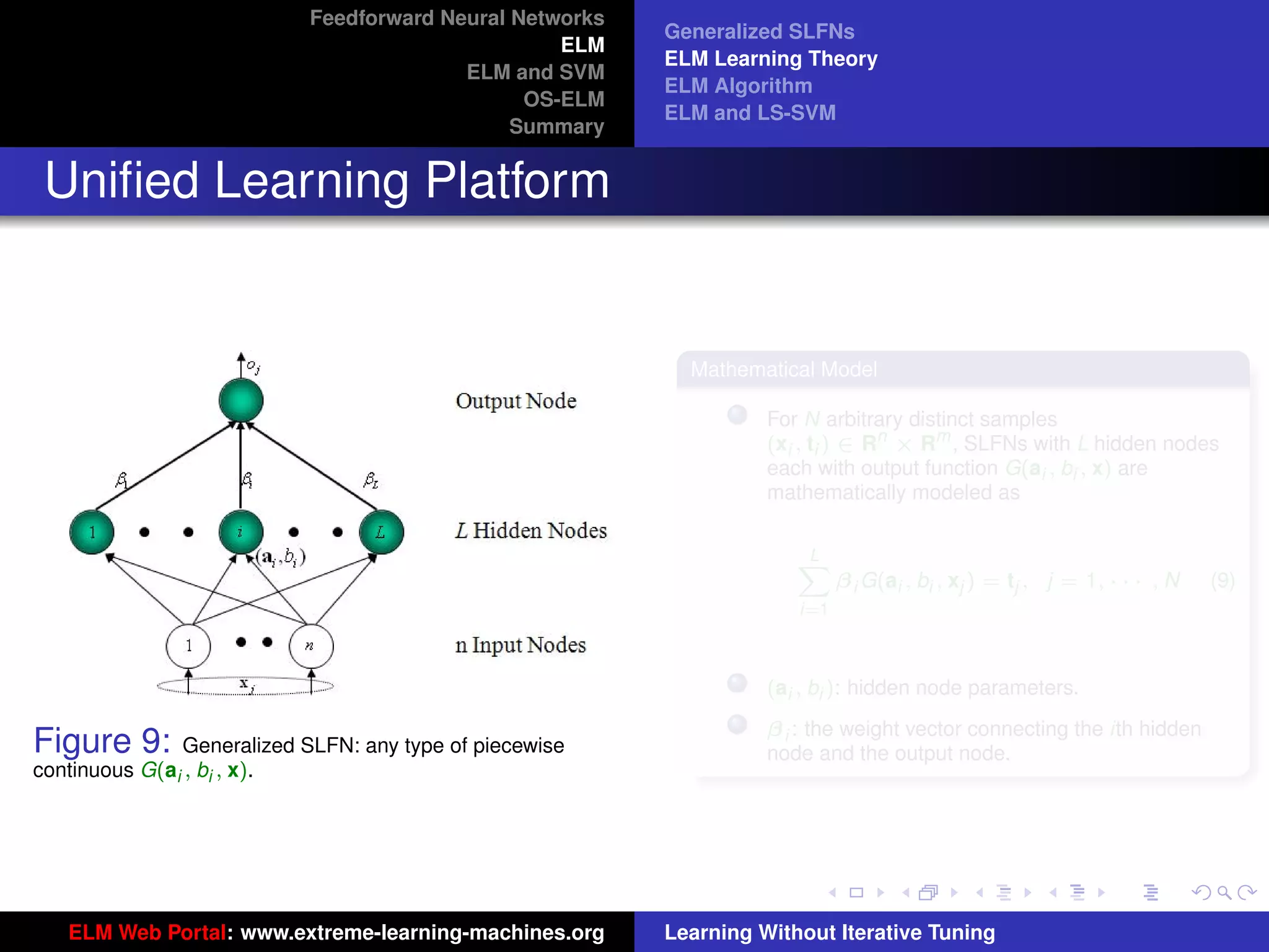
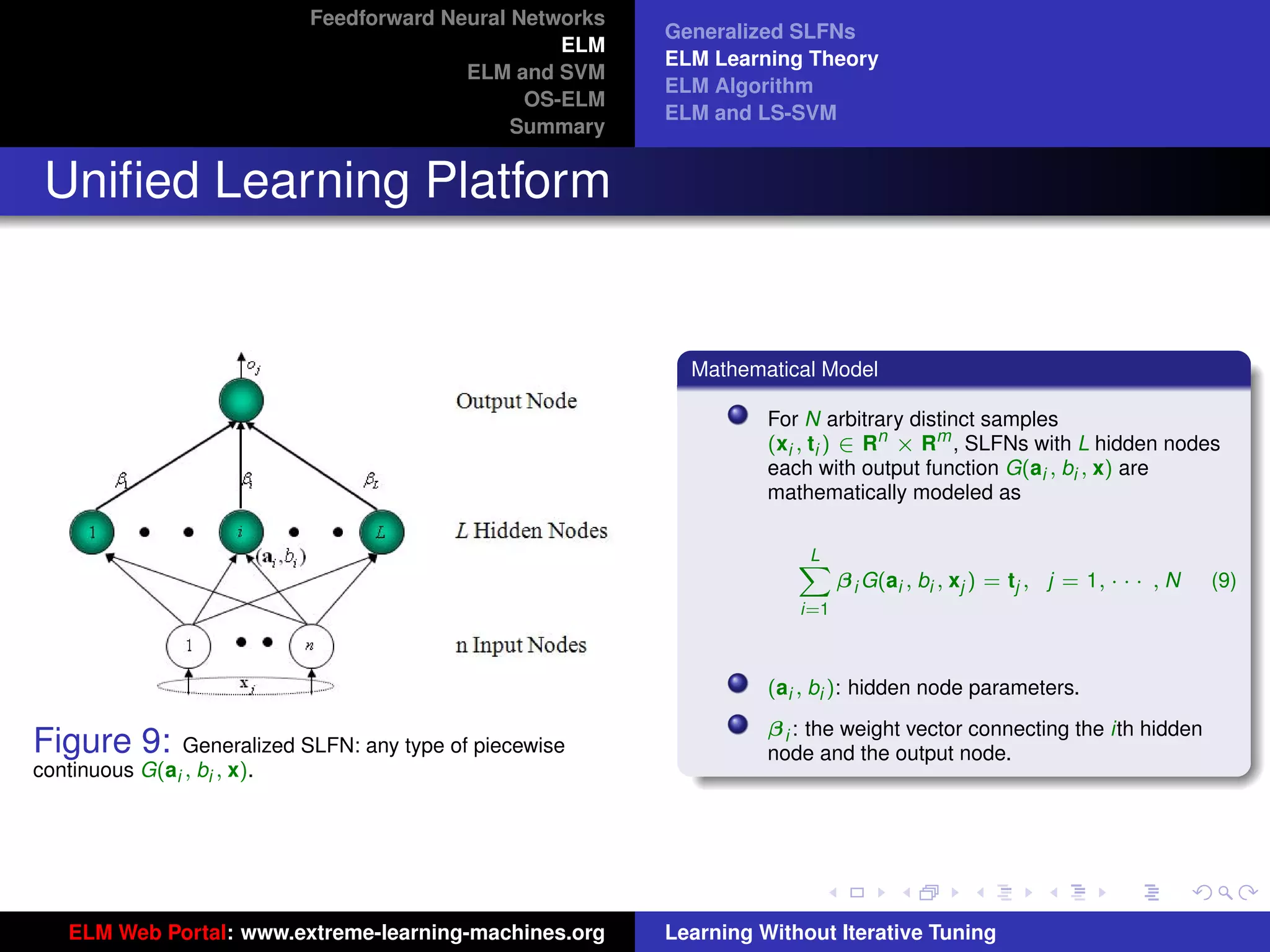
Figure 8: SLFN: any type of piecewise continuous G(ai , bi , x).
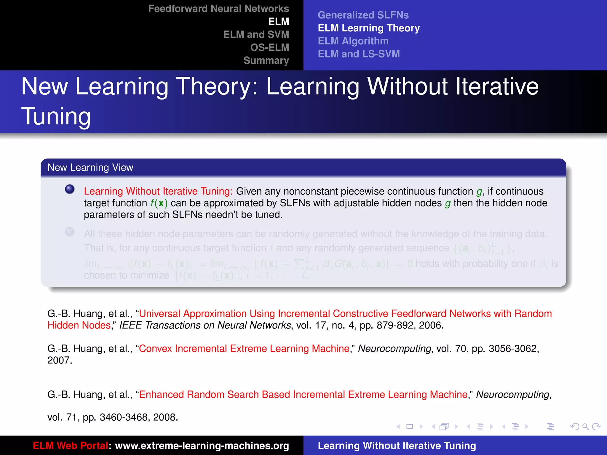
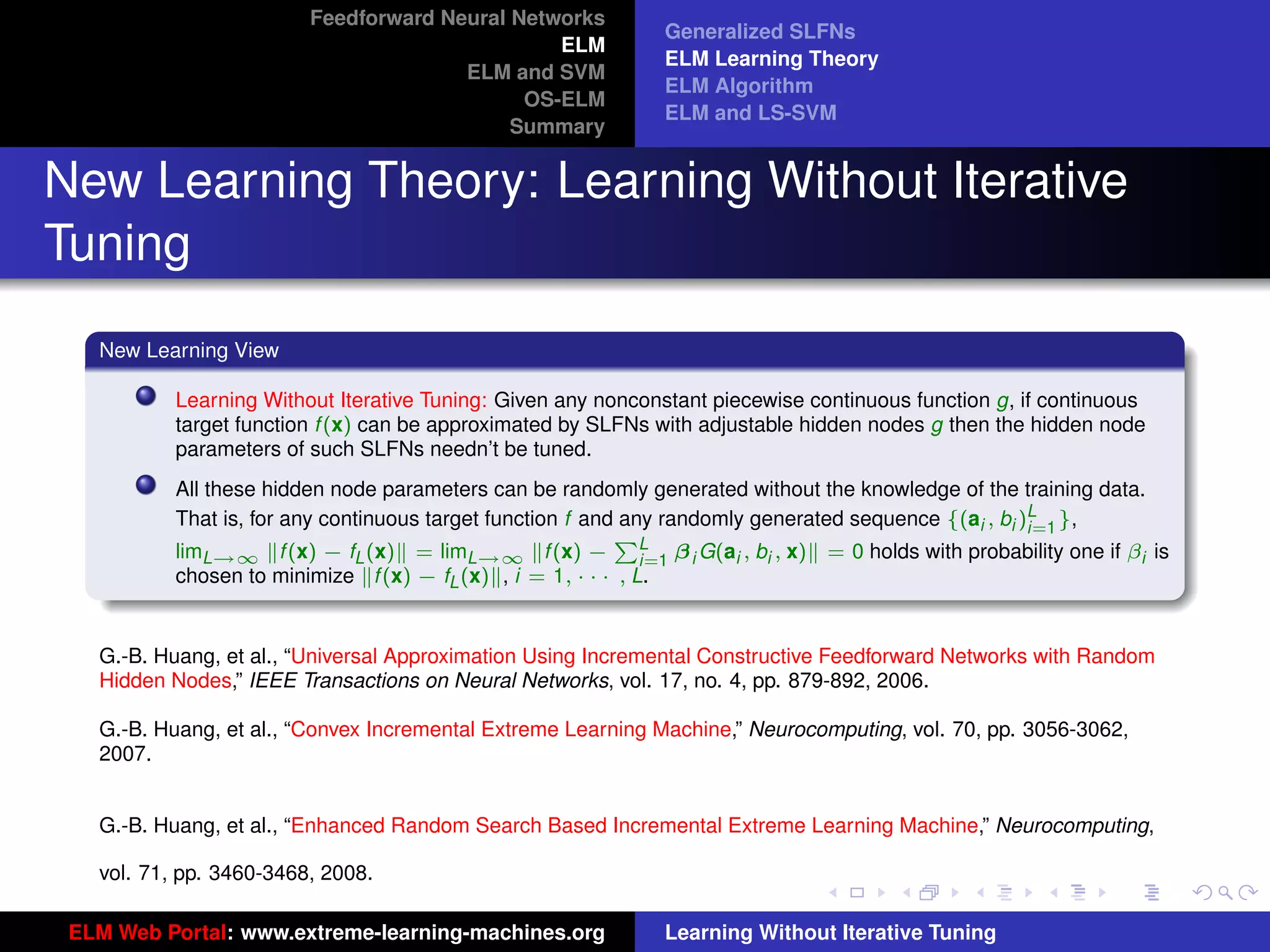
G.-B. Huang, et al., “Universal Approximation Using Incremental Constructive Feedforward Networks with Random tu-logo
Hidden Nodes,” IEEE Transactions on Neural Networks, vol. 17, no. 4, pp. 879-892, 2006.
G.-B. Huang, et al., “Convex Incremental Extreme Learning Machine,” Neurocomputing, vol. 70, pp. 3056-3062, ur-logo
2007.
ELM Web Portal: www.extreme-learning-machines.org Learning Without Iterative Tuning](https://image.slidesharecdn.com/elm-talk-110518005855-phpapp01/75/ELM-Extreme-Learning-Machine-Learning-without-iterative-tuning-33-2048.jpg)
![Feedforward Neural Networks
Generalized SLFNs
ELM
ELM Learning Theory
ELM and SVM
ELM Algorithm
OS-ELM
ELM and LS-SVM
Summary
Generalized SLFNs
General Hidden Layer Mapping
PL
Output function: f (x) = i=1 β i G(ai , bi , x)
The hidden layer output function (hidden layer
mapping):
h(x) = [G(a1 , b1 , x), · · · , G(aL , bL , x)]
The output function needn’t be:
Sigmoid: G(ai , bi , x) = g(ai · x + bi )
RBF: G(ai , bi , x) = g (bi x − ai )
Figure 8: SLFN: any type of piecewise continuous G(ai , bi , x).
G.-B. Huang, et al., “Universal Approximation Using Incremental Constructive Feedforward Networks with Random tu-logo
Hidden Nodes,” IEEE Transactions on Neural Networks, vol. 17, no. 4, pp. 879-892, 2006.
G.-B. Huang, et al., “Convex Incremental Extreme Learning Machine,” Neurocomputing, vol. 70, pp. 3056-3062, ur-logo
2007.
ELM Web Portal: www.extreme-learning-machines.org Learning Without Iterative Tuning](https://image.slidesharecdn.com/elm-talk-110518005855-phpapp01/75/ELM-Extreme-Learning-Machine-Learning-without-iterative-tuning-34-2048.jpg)
![Feedforward Neural Networks
ELM
ELM and SVM
OS-ELM
Summary
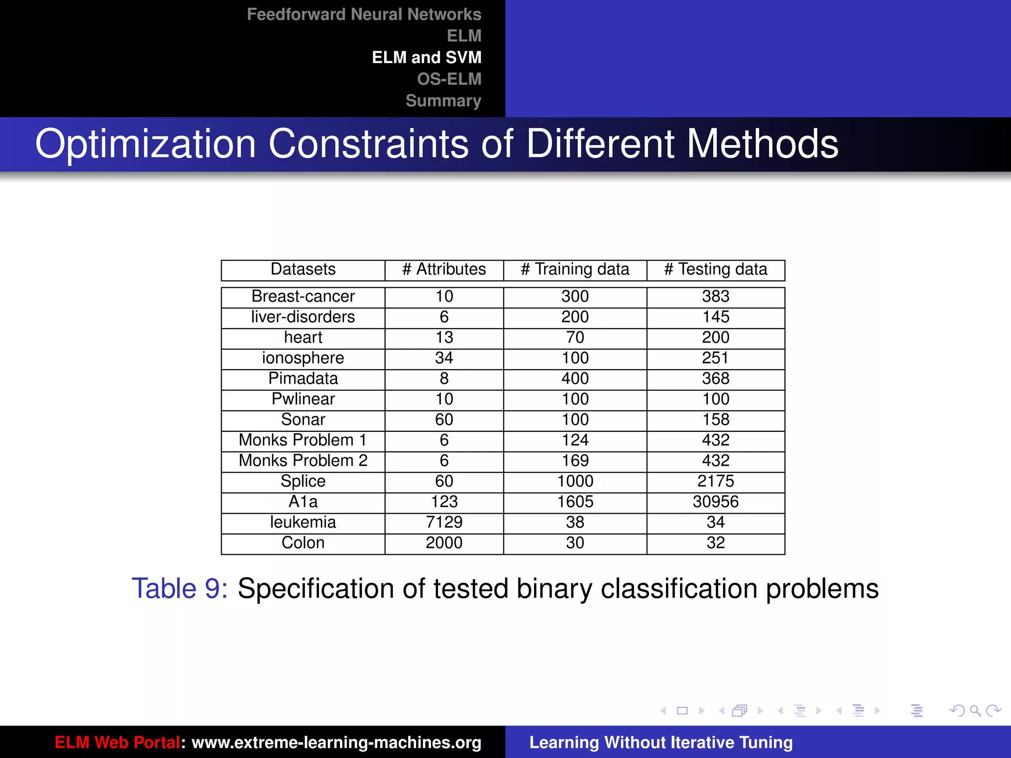
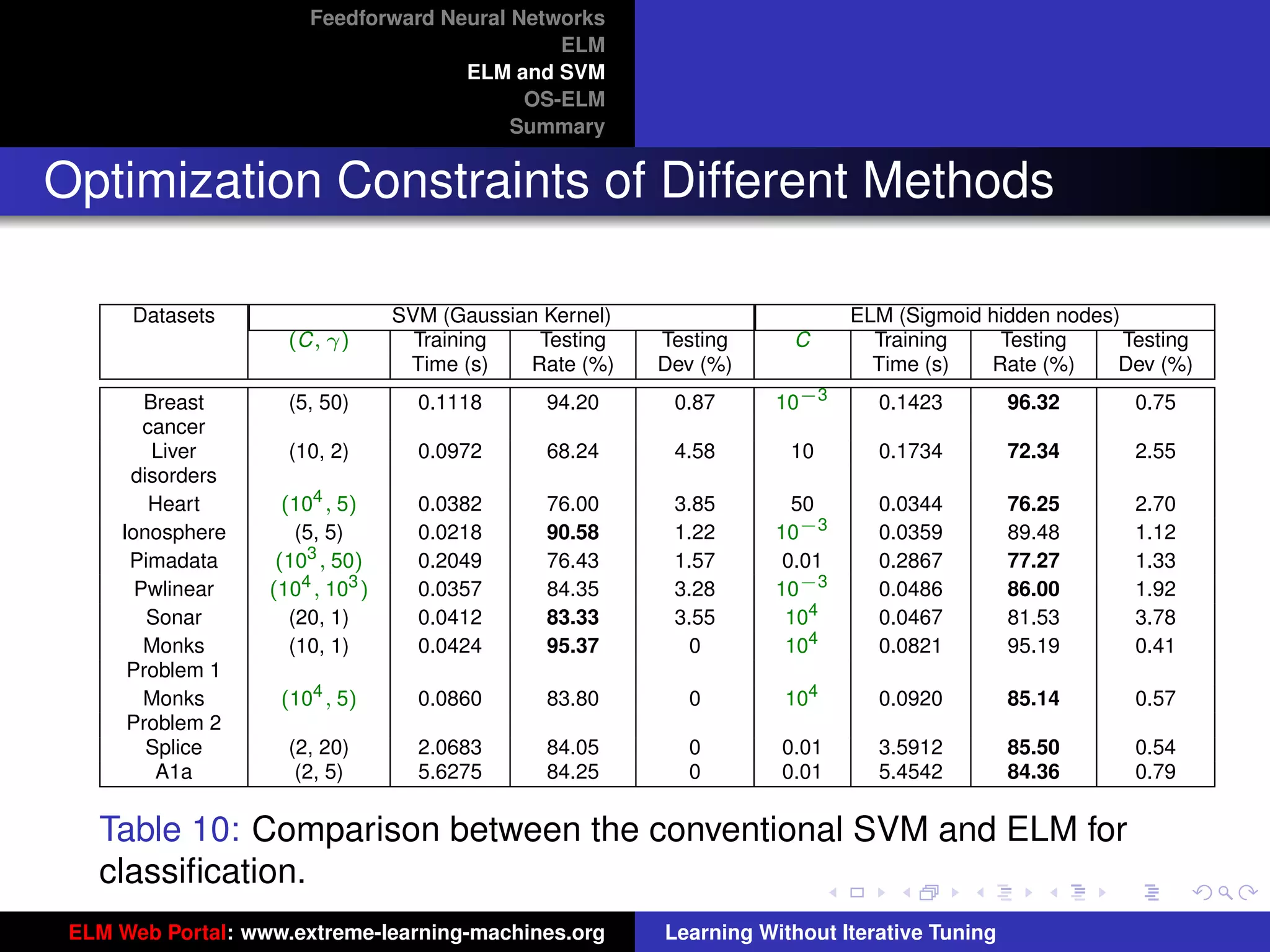
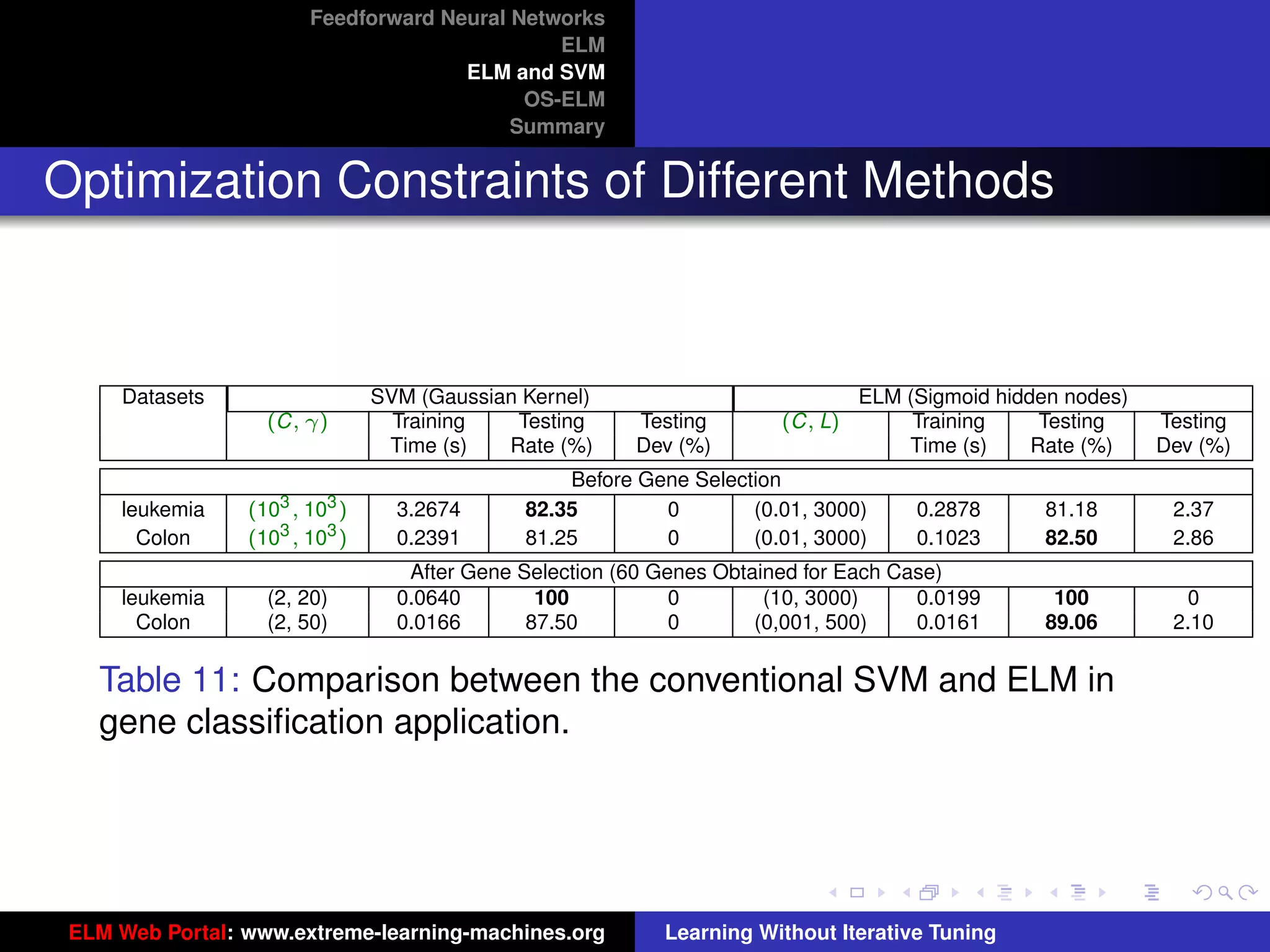
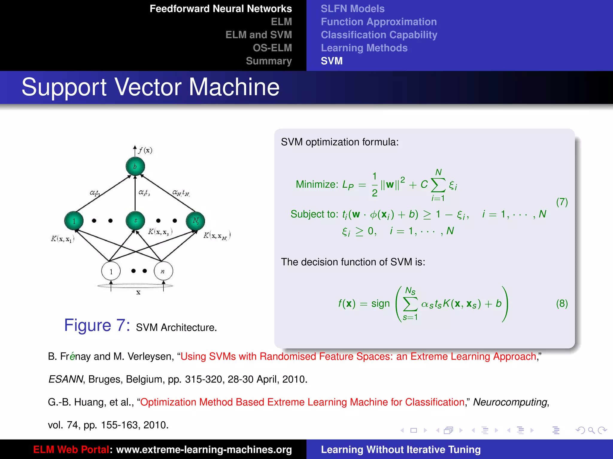
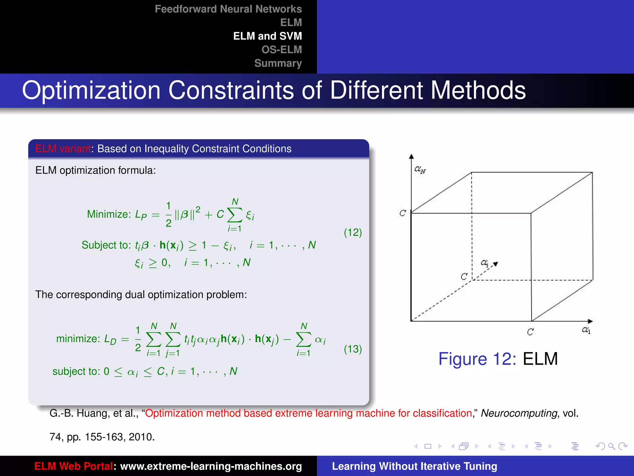
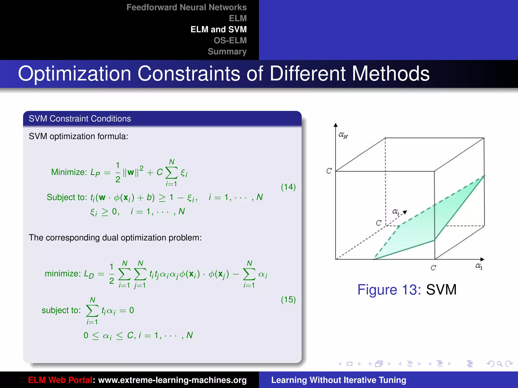
Optimization Constraints of Different Methods
tu-logo
Figure 14: ELM Figure 15: SVM
ELM and SVM have the same dual optimization objective functions, but in ELM optimal αi are found from the entire
ur-logo
cube [0, C]N while in SVM optimal αi are found from one hyperplane
PN
i=1 ti αi = 0 within the cube [0, C]N . SVM
always provides a suboptimal solution, so does LS-SVM.
ELM Web Portal: www.extreme-learning-machines.org Learning Without Iterative Tuning](https://image.slidesharecdn.com/elm-talk-110518005855-phpapp01/75/ELM-Extreme-Learning-Machine-Learning-without-iterative-tuning-69-2048.jpg)
![Feedforward Neural Networks
ELM
ELM and SVM
OS-ELM
Summary
Flaws in SVM Theory?
Flaws?
1 SVM is great! Without SVM computational intelligence may not be so
successful! Many applications and products may not be so successful
either! However ...
2 SVM always searches for the optimal solution in the hyperplane
PN N
i=1 αi ti = 0 within the cube [0, C] of the SVM feature space.
3 Irrelevant applications may be handled similarly in SVMs. Given two
(1) (1) (2) (2) (1) N
training datasets {(xi , ti )}N and {(xi
i=1 , ti )}N and {(xi
i=1 }i=1
(2) (1) (1)
and {(xi }Ni=1 are totally irrelevant/independent, if [t1 , · · · , tN ]T is
(2) (2)
similar or close to [t1 , · · · , tN ]T SVM may have similar search areas
of the cube [0, C]N for two different cases.
G.-B. Huang, et al., “Optimization method based extreme learning machine for Figure 16: SVM
classification,” Neurocomputing, vol. 74, pp. 155-163, 2010.
tu-logo
Reasons
SVM is too “generous” on the feature mappings and kernels, almost condition free except for Mercer’s conditions.
ur-logo
1 As the feature mappings and kernels need not satisfy universal approximation condition, b must be present.
2 As b exists, contradictions are caused.
ELM Web Portal: www.extreme-learning-machines.org Learning Without Iterative Tuning](https://image.slidesharecdn.com/elm-talk-110518005855-phpapp01/75/ELM-Extreme-Learning-Machine-Learning-without-iterative-tuning-70-2048.jpg)
![Feedforward Neural Networks
ELM
ELM and SVM
OS-ELM
Summary
Flaws in SVM Theory?
Flaws?
1 SVM is great! Without SVM computational intelligence may not be so
successful! Many applications and products may not be so successful
either! However ...
2 SVM always searches for the optimal solution in the hyperplane
PN N
i=1 αi ti = 0 within the cube [0, C] of the SVM feature space.
3 Irrelevant applications may be handled similarly in SVMs. Given two
(1) (1) (2) (2) (1) N
training datasets {(xi , ti )}N and {(xi
i=1 , ti )}N and {(xi
i=1 }i=1
(2) (1) (1)
and {(xi }Ni=1 are totally irrelevant/independent, if [t1 , · · · , tN ]T is
(2) (2)
similar or close to [t1 , · · · , tN ]T SVM may have similar search areas
of the cube [0, C]N for two different cases.
G.-B. Huang, et al., “Optimization method based extreme learning machine for Figure 16: SVM
classification,” Neurocomputing, vol. 74, pp. 155-163, 2010.
tu-logo
Reasons
SVM is too “generous” on the feature mappings and kernels, almost condition free except for Mercer’s conditions.
ur-logo
1 As the feature mappings and kernels need not satisfy universal approximation condition, b must be present.
2 As b exists, contradictions are caused.
ELM Web Portal: www.extreme-learning-machines.org Learning Without Iterative Tuning](https://image.slidesharecdn.com/elm-talk-110518005855-phpapp01/75/ELM-Extreme-Learning-Machine-Learning-without-iterative-tuning-71-2048.jpg)