Downloaded 169 times
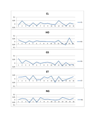
![The result is obviously completely different, in all the cases the null hypothesis is rejected and the series are stationary and non-integrated.
The AR models are normally used to study stationary time series, when we speak of multi- variate time series models we refer to VAR (Vector Auto-Regression) models.
We will now use VAR models to analyze the returns of the five energy futures.
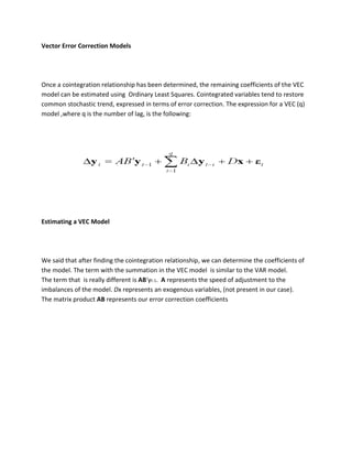
Vector Autoregressive Models
VAR is a simple and useful model for modeling our vectors of returns . We will think in terms of a model like the following:
Yt is a vector [n:1] e A is a [n:n] matrix of the coefficients of the lagged variable Yp . In this case the lag of the model is equal to 1.
Determining an appropriate number of lags
Among the various methods to derive the most appropriate number of lags, we will use Akaike Information Criterion, which requires various values : the likelihood and the number of active parameters in the model.
In practice, we can quickly obtain these data modeling our VAR for different lag (1,2,3,4 ...), keeping in mind that the first values are the most likely. To obtain the likelihood in Matlab, simply type LLF after the estimate of the model parameters. To derive the number of active parameters:
[NumParam,NumActive]=vgxcount( Model name )
To calculate Akaike Information Criterion
AIC = aicbic([LLF1, ...LLFn],[Np1,...Npn])
where LLF indicates the likelihood and Npn indicates the nth number of active parameters.](https://image.slidesharecdn.com/multivariatetimeseries-141214155831-conversion-gate02/85/Multivariate-time-series-6-320.jpg)
![The lowest values of the AIC indicates the best lag.
VAR(p)
Likelihood
NumParam
AIC
1
1.5890e+004
5
-31770
2
1.5936e+004
5
-31862
3
1.6109e+004
5
-32208
4
1.6188e+004
5
-32366
Obviously, we will choose a VAR (1), model, ie with lag equal to one.
VAR(1) Parameters Estimation
In order to estimate the model using Matlab we will follow the following steps:
1. import stationary time series, collected in a matrix in excel with a series of returns in each of the columns and a number of rows equal to the observations.
2. Create the VAR model
We want to build a VAR model with one lag , a constant and five series:
Model = vgxset('n',5,'nAR',1,'Constant',true)
3. Fit the model to the data
We also want to find the values of the constants, parameters and of the covariances of the innovations:
[EstSpec,EstStdErrors,LLF,W] = vgxvarx(Model, DataMatrix);
and obviously we want to see the results
vgxdisp(EstSpec,EstStdErrors)
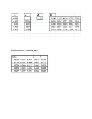
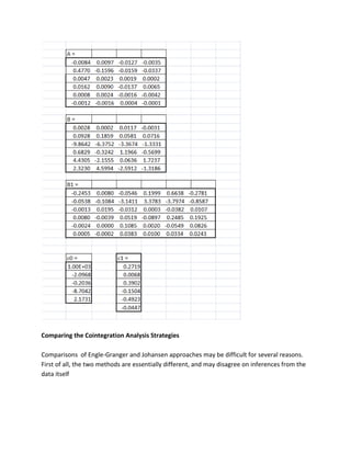
Then we obtain the estimates of the parameters:](https://image.slidesharecdn.com/multivariatetimeseries-141214155831-conversion-gate02/85/Multivariate-time-series-7-320.jpg)
![and the covariance matrix of the residuals
Stability Check
Once fitted the model, we can control the stability of the model, given that we have no MA elements, having only AR model, the model is invertible by definition.
[isStable, isInvertible] = vgxqual(Model);
The answer is a logical operator (0.1) which represent the rejection and acceptance of the hypothesis of stability and reversibility.](https://image.slidesharecdn.com/multivariatetimeseries-141214155831-conversion-gate02/85/Multivariate-time-series-8-320.jpg)
![In our case the answer (ans) is: (1.1). The model is stable and invertible.
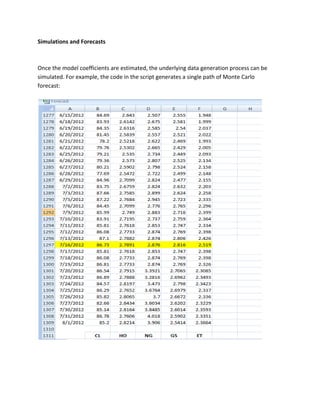
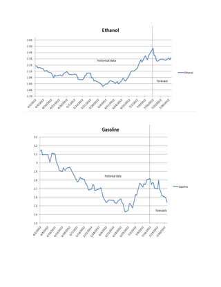
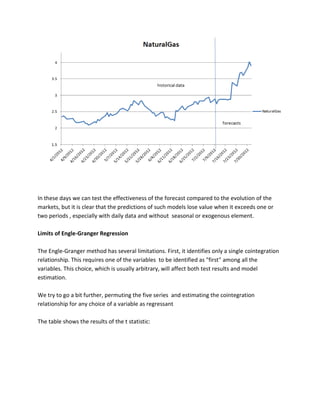
Forecasts using a VAR model
We can use the estimated VAR model to make predictions about future values of the series studied.
[ypred,ycov] = vgxpred(Model, [],5,[],[])
Is an iterative instruction that uses the model we built and estimated to make 5 predictions about future changes in the futures prices.](https://image.slidesharecdn.com/multivariatetimeseries-141214155831-conversion-gate02/85/Multivariate-time-series-9-320.jpg)
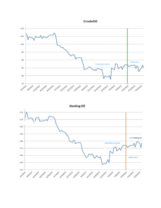
![We could check , later in this project, whether these changes are consistent with the forecasts of our VEC models on closing prices .
Closing Prices Time Series
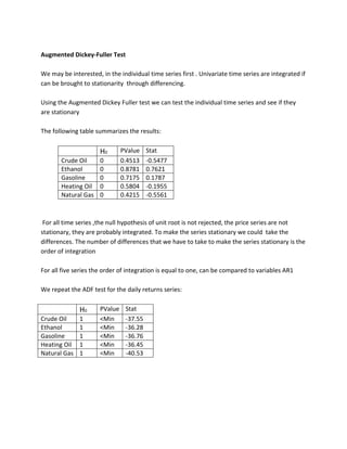
We have already seen, with the ADF tests, that time series of prices are not stationary. We want a confirmation from the KPSS test, which evaluates the null hypothesis that a univariate time series y is trend stationary against the alternative that it is a unit root . We want this series to be integrated.
[h0,pVal0] = kpsstest(TimeSeries,'trend',false)
KPSS Test
H0
PValue
Crude Oil
1
>0.01
Ethanol
1
>0.01
Gasoline
1
>0.01
Heating Oil
1
>0.01
Natural Gas
1
>0.01
The results show that we accept the hypothesis that the processes are integrated in all the time series of derivative prices. We may calculate the order of integration of each series obtaining the number of differences required to make the series stationary.
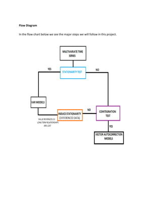
Returning to the flowchart, rejecting the hypothesis of stationarity and having an indication of integrated processes, we continue in the right part of the scheme and apply a first test of cointegration.](https://image.slidesharecdn.com/multivariatetimeseries-141214155831-conversion-gate02/85/Multivariate-time-series-11-320.jpg)
![Engle-Granger Test for Cointegration
To get information about the presence of a cointegration relationship, we will run the Engle- Granger test and T-test, this time over the entire Matrix of our futures prices.
The test has the form:
Y(:,1)=Y(:2:end)*b+X+a+e
On the left side we have the regressand , the first series, while on the right-side ofthe equation , from 2 to five in our case, we have the regressors. The key factor here are the residuals, to be more precise, the estimates of residuals. If the residuals series is stationary, the linear combination of variables is stationary
[hEG,pValEG]=egtest(DataMatrix,'test',{'t1})
we obtain the following results:
H0
PValue
t
Engle-Granger
1
0.0615
---
t.statistic
1
----
0.1
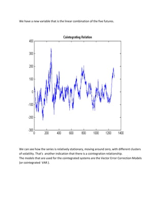
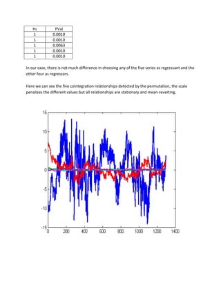
Both tests indicate the presence of cointegration in the matrix of the values of the derivatives. At this point, we want to identify the cointegration relationship.
We extract the vector of parameter b and the intercept c0 obtained running the function egcitest and form a linear combination of regression:
c0=reg.coeff(1);
b=reg.coeff(2:5);
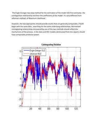
plot(Y*[1;-b]-c0,'LineWidth',2)](https://image.slidesharecdn.com/multivariatetimeseries-141214155831-conversion-gate02/85/Multivariate-time-series-12-320.jpg)
![Another limitation of the Engle-Granger method is that it is a two-steps procedure, with a first regression that estimates the residual series, and another regression to verify the unit root. Errors in the initial estimate are necessarily brought in the second evaluation.
Furthermore, the Engle-Granger method for the estimation of the cointegration relationships play a role in the VEC model definition. As a result, the VEC model estimates also becomes a two-step procedure
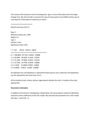
Johansen Test for Cointegration
The Johansen test for cointegration addresses many of the limitations of the Engle-Granger method. It avoids the two-step estimators and provides comprehensive tests in the presence of multiple cointegrating relationships.
His approach incorporates the maximum-likelihood test procedure in the process of estimating the model, avoiding conditional estimates. Furthermore, the test provides a framework for testing restrictions on cointegrating relationships.
The key point in the Johansen method is the ratio between the degree of the impact matrix
C = AB' and the size of its eigenvalues. The eigenvalues depend on the shape of the VEC model, and in particular on the composition of its deterministic terms. The method relies on the rank of cointegration by testing the number of eigenvalues that are statistically different from 0.
We will now run the test for the cointegration rank using the H1 default model,the form of the H1 model is:
A(B'yt-1+C0)+C1
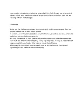
[~,~,~,~,mles] = jcitest(Y,'model','H1','lags',2,'display','params');
The term mLes refers to the fact that the test procedure is based on the Maximum Likelihood method.](https://image.slidesharecdn.com/multivariatetimeseries-141214155831-conversion-gate02/85/Multivariate-time-series-21-320.jpg)

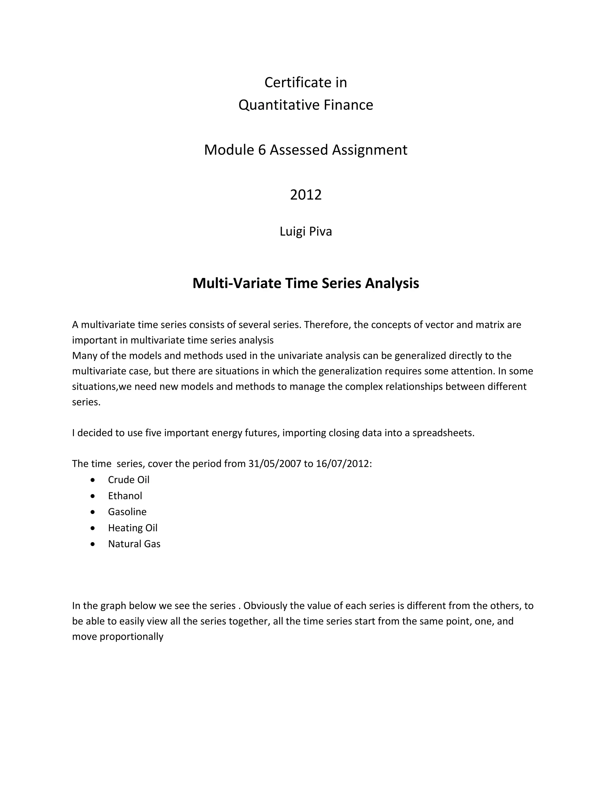
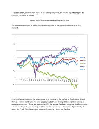
The document discusses analyzing multivariate time series of five energy futures (crude oil, ethanol, gasoline, heating oil, natural gas) using vector autoregressive (VAR) and vector error correction (VEC) models. It finds the futures are cointegrated using Johansen and Engle-Granger tests, indicating they share a common stochastic trend. A VAR(1) model is estimated and found stable. The VEC model captures the error correction behavior as futures return to their long-run equilibrium. Forecasts are generated and limitations of the Engle-Granger approach discussed.


