Frequency Response with MATLAB Examples.pdf

Frequency Response
with MATLAB Examples
Control Design and Analysis
https://www.halvorsen.blog
Hans-Petter Halvorsen

Contents
• Introduction to PID Control
• Introduction to Frequency Response
• Frequency Response using Bode Diagram
• Introduction to Complex Numbers (which Frequency Response Theory is
based on)
• Frequency Response from Transfer Functions
• Frequency Response from Input/output Signals
• PID Controller Design and Tuning (Theory)
• PID Controller Design and Tuning using MATLAB
• Stability Analysis using MATLAB
• Stability Analysis of Feedback Systems
• Stability Analysis of Feedback Systems – a Practical Example
• The Bandwidth of the Control System
• Practical PI Controller Example

PID Control

Control System
𝑟 – Reference Value, SP (Set-point), SV (Set Value)
𝑦 – Measurement Value (MV), Process Value (PV)
𝑒 – Error between the reference value and the measurement value (𝑒 = 𝑟 – 𝑦)
𝑣 – Disturbance, makes it more complicated to control the process
𝑢 - Control Signal from the Controller
Controller Process
Sensors
Actuators
Filtering
𝑟 𝑢
𝑒
− 𝑦
𝑣

The PID Algorithm
Tuning Parameters:
𝐾𝑝
𝑇𝑖
𝑇𝑑
Where 𝑢 is the controller output and 𝑒 is the
control error:
𝑒 𝑡 = 𝑟 𝑡 − 𝑦(𝑡)
𝑟 is the Reference Signal or Set-point
𝑦 is the Process value, i.e., the Measured value
𝑢 𝑡 = 𝐾𝑝𝑒 +
𝐾𝑝
𝑇𝑖
න
0
𝑡
𝑒𝑑𝜏 + 𝐾𝑝𝑇𝑑 ሶ
𝑒
Proportional Gain
Integral Time [sec. ]
Derivative Time [sec. ]

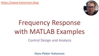
The PI Algorithm
Tuning Parameters:
𝐾𝑝
𝑇𝑖
Where 𝑢 is the controller output and 𝑒 is the
control error:
𝑒 𝑡 = 𝑟 𝑡 − 𝑦(𝑡)
𝑟 is the Reference Signal or Set-point
𝑦 is the Process value, i.e., the Measured value
𝐾𝑝
𝑇𝑖
න
0
𝑡
𝑒𝑑𝜏
Proportional Gain
Integral Time [sec. ]

PI(D) Algorithm in MATLAB
• We can use the pid() function in MATLAB
• We can define the PI(D) transfer function
using the tf() function in MATLAB
• We can also define and implement a discrete
PI(D) algorithm

Discrete PI Controller Algorithm
We start with:
𝑢 𝑡 = 𝑢0 + 𝐾𝑝𝑒 𝑡 +
𝐾𝑝
𝑇𝑖
න
0
𝑡
𝑒𝑑𝜏
In order to make a discrete version using, e.g., Euler, we can derive both sides of the equation:
ሶ
𝑢 = ሶ
𝑢0 + 𝐾𝑝 ሶ
𝑒 +
𝐾𝑝
𝑇𝑖
𝑒
If we use Euler Forward we get:
𝑢𝑘 − 𝑢𝑘−1
𝑇𝑠
=
𝑢0,𝑘 − 𝑢0,𝑘−1
𝑇𝑠
+ 𝐾𝑝
𝑒𝑘 − 𝑒𝑘−1
𝑇𝑠
+
𝐾𝑝
𝑇𝑖
𝑒𝑘
Then we get:
𝑢𝑘 = 𝑢𝑘−1 + 𝑢0,𝑘 − 𝑢0,𝑘−1 + 𝐾𝑝 𝑒𝑘 − 𝑒𝑘−1 +
𝐾𝑝
𝑇𝑖
𝑇𝑠𝑒𝑘
Where
𝑒𝑘 = 𝑟𝑘 − 𝑦𝑘
We can also split the equation above in 2 different parts by setting:
∆𝑢𝑘 = 𝑢𝑘 − 𝑢𝑘−1
This gives the following PI control algorithm:
∆𝑢𝑘 = 𝑢0,𝑘 − 𝑢0,𝑘−1 + 𝐾𝑝 𝑒𝑘 − 𝑒𝑘−1 +
𝐾𝑝
𝑇𝑖
𝑇𝑠𝑒𝑘
𝑢𝑘 = 𝑢𝑘−1 + ∆𝑢𝑘
This algorithm can easily be implemented in MATLAB

Discrete PI Controller Algorithm
∆𝑢𝑘 = 𝑢0,𝑘 − 𝑢0,𝑘−1 + 𝐾𝑝 𝑒𝑘 − 𝑒𝑘−1 +
𝐾𝑝
𝑇𝑖
𝑇𝑠𝑒𝑘
𝑢𝑘 = 𝑢𝑘−1 + ∆𝑢𝑘
Discrete PI control algorithm:

PID Controller –Transfer Function
𝐾𝑝
𝑇𝑖
න
0
𝑡
𝑒𝑑𝜏 + 𝐾𝑝𝑇𝑑 ሶ
𝑒
Laplace gives:
We have:
𝐻𝑃𝐼𝐷 𝑠 =
𝑢(𝑠)
𝑒(𝑠)
= 𝐾𝑝 +
𝐾𝑝
𝑇𝑖𝑠
+ 𝐾𝑝𝑇𝑑𝑠
or:
𝐻𝑃𝐼𝐷 𝑠 =
𝑢(𝑠)
𝑒(𝑠)
=
𝐾𝑝(𝑇𝑑𝑇𝑖𝑠2 + 𝑇𝑖𝑠 + 1)
𝑇𝑖𝑠

PI Controller –Transfer Function
𝐻𝑃𝐼 𝑠 =
𝑢(𝑠)
𝑒(𝑠)
=
𝐾𝑝(𝑇𝑖𝑠 + 1)
𝑇𝑖𝑠
𝐾𝑝
𝑇𝑖
න
0
𝑡
𝑒𝑑𝜏
Laplace gives:
We have:
𝐻𝑃𝐼 𝑠 =
𝑢(𝑠)
𝑒(𝑠)
= 𝐾𝑝 +
𝐾𝑝
𝑇𝑖𝑠
=
𝐾𝑝𝑇𝑖𝑠 + 𝐾𝑝
𝑇𝑖𝑠
=
𝑇𝑖𝑠
Finally:

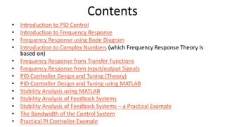
Define PI Transfer function in MATLAB
clear, clc
% PI Controller Transfer function
Kp = 0.52;
Ti = 18;
num = Kp*[Ti, 1];
den = [Ti, 0];
Hpi = tf(num,den)
...
𝐻𝑃𝐼 𝑠 =
𝑢(𝑠)
𝑒(𝑠)
=
𝑇𝑖𝑠

PI Controller – State space model
Given:
𝑢 𝑠 = 𝐾𝑝𝑒 𝑠 +
𝐾𝑝
𝑇𝑖𝑠
𝑒 𝑠
We set 𝑧 =
1
𝑠
𝑒 ⇒ 𝑠𝑧 = 𝑒 ⇒ ሶ
𝑧 = 𝑒
This gives:
ሶ
𝑧 = 𝑒
𝑢 = 𝐾𝑝𝑒 +
𝐾𝑝
𝑇𝑖
𝑧
Where
𝑒 = 𝑟 − 𝑦

PI Controller – Discrete State space model
Using Euler:
ሶ
𝑧 ≈
𝑧𝑘+1 − 𝑧𝑘
𝑇𝑠
Where 𝑇𝑠 is the Sampling Time.
This gives:
𝑧𝑘+1 − 𝑧𝑘
𝑇𝑠
= 𝑒𝑘
𝑢𝑘 = 𝐾𝑝𝑒𝑘 +
𝐾𝑝
𝑇𝑖
𝑧𝑘
Finally:
𝑢𝑘 = 𝐾𝑝𝑒𝑘 +
𝐾𝑝
𝑇𝑖
𝑧𝑘
𝑧𝑘+1 = 𝑧𝑘 + 𝑇𝑠𝑒𝑘

PI Controller – Discrete State space model
implemented in MATLAB clear, clc
...
for i=1:N
...
e = r - y;
u = Kp*e + z;
z = z + dt*Kp*e/Ti;
...
end
plot(...)

Frequency Response

Frequency Response
• The frequency response of a system is a frequency dependent
function which expresses how a sinusoidal signal of a given frequency
on the system input is transferred through the system. Each
frequency component is a sinusoidal signal having certain amplitude
and a certain frequency.
• The frequency response is an important tool for analysis and design
of signal filters and for analysis and design of control systems.
• The frequency response can be found experimentally or from a
transfer function model.
• The frequency response of a system is defined as the steady-state
response of the system to a sinusoidal input signal. When the system
is in steady-state, it differs from the input signal only in
amplitude/gain (A) and phase lag (𝜙).
Theory

Frequency
Response
Dynamic
System
Input Signal
Output Signal
Gain Phase Lag
Frequency
Amplitude
The frequency response of a system expresses how a sinusoidal signal of a given frequency on the system
input is transferred through the system. The only difference is the gain and the phase lag.
Theory
𝑢 𝑡 = 𝑈 ∙ 𝑠𝑖𝑛𝜔𝑡
𝑦 𝑡 = ด
𝑈𝐴
𝑌
𝑠𝑖𝑛(𝜔𝑡 + 𝜙)
Input Signal
Output Signal

Frequency Response - Definition
• The frequency response of a system is defined as the steady-state response of the system to a sinusoidal
input signal.
• When the system is in steady-state, it differs from the input signal only in amplitude/gain (A) (Norwegian:
“forsterkning”) and phase lag (ϕ) (Norwegian: “faseforskyvning”).
and the same for Frequency 2, 3, 4, 5, 6, etc.
Theory
𝑢 𝑡 = 𝑈 ∙ 𝑠𝑖𝑛𝜔𝑡 𝑦 𝑡 = ด
𝑈𝐴
𝑌
Dynamic
System
𝜔 = 1 𝑟𝑎𝑑/𝑠
𝜔 = 1 𝑟𝑎𝑑/𝑠
Input Output

Frequency Response - Simple Example
Inside Temperature
Assume the outdoor temperature is varying like a sine function during a year (frequency 1) or during 24 hours (frequency 2).
Then the indoor temperature will be a sine as well, but with different gain. In addition it will have a phase lag.
Note! Only the
gain and phase
are different
Theory
Outside Temperature
Dynamic System
frequency 1 (year)
T = 1 year
frequency 1 (year)

Frequency Response - Simple Example
Inside Temperature
Assume the outdoor temperature is varying like a sine function during a year (frequency 1) or during 24 hours (frequency 2).
Then the indoor temperature will be a sine as well, but with different gain. In addition it will have a phase lag.
Note! Only the gain and phase are different
Theory
Outside Temperature
Dynamic System frequency 2 (24 hours)
frequency 2 (24 hours)
T = 24 hours

Frequency Response using
Bode Diagram

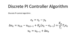
Bode Diagram
𝐿𝑜𝑔 𝜔
𝐿𝑜𝑔 𝜔
𝜑
∆𝐾
𝜔𝑐
𝜔180
You can find the Bode diagram from experiments on the physical process or from the transfer function (the model of the
system). A simple sketch of the Bode diagram for a given system:
The Bode diagram gives a simple Graphical
overview of the Frequency Response for a
given system. A Tool for Analyzing the
Stability properties of the Control System.
With MATLAB you can easily create Bode
diagram from the Transfer function model
using the bode() function
ω [rad/s]
ω [rad/s]
0𝑑𝐵

Bode Diagram from experiments
We find 𝐴 and 𝜙 for each of the frequencies,
e.g.:
Based on that we can plot the
Frequency Response in a so-called Bode
Diagram:
Find Data for different frequencies
...

Bode Diagram The x-scale is logarithmic
Gain (“Forsterkningen”)
Phase lag (“Faseforkyvningen”)
Note! The y-scale is in [𝑑𝐵]
Normally, the unit for frequency is Hertz [Hz], but in frequency response and Bode
diagrams we use radians ω [rad/s]. The relationship between these are as follows:
The y-scale is in [𝑑𝑒𝑔𝑟𝑒𝑒𝑠]
𝑥 𝑑𝐵 = 20𝑙𝑜𝑔10𝑥
2𝜋 𝑟𝑎𝑑 = 360°
𝜔 = 2𝜋𝑓

Frequency Response – MATLAB
clear
clc
close all
% Define Transfer function
num=[1];
den=[1, 1];
H = tf(num, den)
% Frequency Response
bode(H);
grid on
The frequency response is an important tool for analysis and design
of signal filters and for analysis and design of control systems.
Transfer Function:
MATLAB Code:

Frequency Response – MATLAB
clear
clc
close all
% Define Transfer function
num = [1];
den = [1, 1];
H = tf(num, den)
% Frequency Response
bode(H);
grid on
% Get Freqquency Response Data
wlist = [0.01, 0.1, 1, 2 ,3 ,5 ,10, 100];
[mag, phase, w] = bode(H, wlist);
for i=1:length(w)
magw(i) = mag(1,1,i);
phasew(i) = phase(1,1,i);
end
magdB = 20*log10(magw); % Convert to dB
freq_data = [wlist; magdB; phasew]'
Transfer Function:
Instead of Plotting the Bode Diagram we
can also use the bode function for
calculation and showing the data as well:
freq_data =
0.0100 -0.0004 -0.5729
0.1000 -0.0432 -5.7106
1.0000 -3.0103 -45.0000
2.0000 -6.9897 -63.4349
3.0000 -10.0000 -71.5651
5.0000 -14.1497 -78.6901
10.0000 -20.0432 -84.2894
100.0000 -40.0004 -89.4271

Bode Diagram – MATLAB Example
clear, clc
% Transfer function
num=[1];
den1=[1,0];
den2=[1,1]
den3=[1,1]
den = conv(den1,conv(den2,den3));
H = tf(num, den)
% Bode Diagram
bode(H)
subplot(2,1,1)
grid on
subplot(2,1,2)
grid on
clear, clc
% Transfer function
num=[1];
den=[1,2,1,0];
H = tf(num, den)
% Bode Diagram
bode(H)
subplot(2,1,1)
grid on
subplot(2,1,2)
grid on
or:
MATLAB Code:

Example
We will use the following system as an example:
𝐻𝑐 = 𝐾𝑝
𝐻𝑝 =
1
𝑠(𝑠 + 1)
𝐻𝑚 =
1
3𝑠 + 1
Controller Process
Sensors
𝑟 𝑢
𝑒
− 𝑦

Bode Diagram – MATLAB Example
clear
clc
num = 1;
den = [1,1,0];
Hp = tf(num,den)
bode(Hp)
grid on
MATLAB Code:
𝐻𝑝 =
1
𝑠(𝑠 + 1)

Complex Numbers
Background Theory for Frequency Response

A Complex Number is given by:
𝑧 = 𝑎 + 𝑗𝑏
Where
𝑗 = −1
We have that:
𝑎 = 𝑅𝑒 𝑧
𝑏 = 𝐼𝑚(𝑧)
Complex Numbers
0 𝑎
𝑏
𝐼𝑚𝑎𝑔𝑖𝑛𝑎𝑟𝑦
𝐴𝑥𝑖𝑠 (𝐼𝑚)
𝑅𝑒𝑎𝑙
𝐴𝑥𝑖𝑠(𝑅𝑒)

Complex Numbers
Polar form:
𝑧 = 𝑟𝑒𝑗𝜃
Where:
𝑟 = 𝑧 = 𝑎2+𝑏2
𝜃 = 𝑎𝑡𝑎𝑛
𝑏
𝑎
Note!
𝑎 = 𝑟 cos 𝜃
𝑏 = 𝑟 sin 𝜃
0 𝑎
𝑏
𝑅𝑒𝑎𝑙
𝜃
𝑟
𝑗 = −1

Complex Numbers
Rectangular form of a complex number Exponential/polar form of a complex number
Length (“Gain”): Angle (“Phase”):
1 2
0 𝑎
𝑏
𝑅𝑒𝑎𝑙
0 𝑎
𝑏
𝑅𝑒𝑎𝑙
𝜃
𝑟
𝑟 = 𝑧 = 𝑎2 + 𝑏2 𝜃 = 𝑎𝑡𝑎𝑛
𝑏
𝑎
𝑗 = −1

Frequency response from
Transfer function

Manually find the Frequency Response
from the Transfer Function
For a transfer function:
𝐻 𝑆 =
𝑦(𝑠)
𝑢(𝑠)
We have that:
𝐻 𝑗𝜔 = 𝐻(𝑗𝜔) 𝑒𝑗∠𝐻(𝑗𝜔)
Where 𝐻(𝑗𝜔) is the frequency response of the system, i.e., we may find the frequency response by setting 𝑠 = 𝑗𝜔
in the transfer function. Bode diagrams are useful in frequency response analysis.
The Bode diagram consists of 2 diagrams, the Bode magnitude diagram, 𝐴(𝜔) and the Bode phase diagram,
𝜙(𝜔).
The Gain function:
𝐴 𝜔 = 𝐻(𝑗𝜔)
The Phase function:
𝜙 𝜔 = ∠𝐻(𝑗𝜔)
The 𝐴(𝜔)-axis is in decibel (dB), where the decibel value of x is calculated as: 𝑥 𝑑𝐵 = 20𝑙𝑜𝑔10𝑥
The 𝜙(𝜔)-axis is in degrees (not radians!)
Theory
𝑠 = 𝑗𝜔

Mathematical expressions for 𝐴(𝜔) and 𝜙(𝜔)
cont. next page
We find the Mathematical expressions for 𝐴(𝜔) and 𝜙(𝜔) by setting 𝑠 = 𝑗𝜔 in the transfer function
given by:
𝐻 𝑠 =
𝑦(𝑠)
𝑢(𝑠)
=
𝐾
𝑇𝑠 + 1
The Frequency Response (we replace 𝑠 with 𝑗𝜔) then becomes:
𝐻 𝑗𝜔 =
𝐾
𝑇𝑗𝜔 + 1
=
𝐾
ณ
1
𝑅𝑒
+ 𝑗 ด
𝑇𝜔
𝐼𝑚
Polar form:
𝐻 𝑗𝜔 =
𝐾
12 + 𝑇𝜔 2𝑒
𝑗 𝑎𝑟𝑐𝑡𝑎𝑛
𝑇𝜔
1
=
𝐾
1 + 𝑇𝜔 2
𝑒𝑗 −𝑎𝑟𝑐𝑡𝑎𝑛(𝑇𝜔)
Finally:
𝐻 𝑗𝜔 =
𝐾
1 + 𝑇𝜔 2
𝑒𝑗 −𝑎𝑟𝑐𝑡𝑎𝑛(𝑇𝜔)

cont. from previous page
The Gain function becomes:
𝐴 𝜔 = 𝐻(𝑗𝜔) =
𝐾
1 + 𝑇𝜔 2
Or in 𝑑𝐵 (used in the Bode Plot):
𝐴 𝜔 𝑑𝐵 = 𝐻(𝑗𝜔) 𝑑𝐵 = 20𝑙𝑜𝑔𝐾 − 20𝑙𝑜𝑔 1 + 𝑇𝜔 2
The Phase function becomes ( 𝑟𝑎𝑑 ):
𝜙 𝜔 = ∠𝐻 𝑗𝜔 = 𝑎𝑟𝑔 𝐻 𝑗𝜔 = −𝑎𝑟𝑐𝑡𝑎𝑛(𝑇𝜔)
Or in degrees ° (used in the Bode plot):
𝜙 𝜔 = ∠𝐻 𝑗𝜔 = −𝑎𝑟𝑐𝑡𝑎𝑛(𝑇𝜔) ∙
180
𝜋
Note: 2𝜋 𝑟𝑎𝑑 = 360°

Transfer function: 𝑨(𝝎) og 𝝓(𝝎):
𝐻 𝑠 =
1
𝑠 + 1
𝐻(𝑗𝜔) 𝑑𝐵 = 20𝑙𝑜𝑔1 − 20𝑙𝑜𝑔 (𝜔)2+1
∠𝐻(𝑗𝜔) = −arctan(𝜔)
𝐻 𝑠 =
4
2𝑠 + 1
𝐻(𝑗𝜔) 𝑑𝐵 = 20𝑙𝑜𝑔4 − 20𝑙𝑜𝑔 (2𝜔)2+1
∠𝐻(𝑗𝜔) = −arctan(2𝜔)
𝐻 𝑆 =
5
𝑠 + 1 (10𝑠 + 1)
𝐻(𝑗𝜔) 𝑑𝐵 = 20𝑙𝑜𝑔5 − 20𝑙𝑜𝑔 (𝜔)2+1 − 20𝑙𝑜𝑔 (10𝜔)2+1
∠𝐻(𝑗𝜔) = −arctan(𝜔) − arctan(10𝜔)
𝐻 𝑆 =
1
𝑠 𝑠 + 1 2
𝐻(𝑗𝜔) 𝑑𝐵 = −20𝑙𝑜𝑔 (𝜔)2− 2𝑥20𝑙𝑜𝑔 (𝜔)2+1
= 20𝑙𝑜𝑔𝜔 − 40𝑙𝑜𝑔 (𝜔)2+1
∠𝐻(𝑗𝜔) = −90 − 2 arctan(𝜔)
𝐻 𝑠 =
3.2𝑒−2𝑠
3𝑠 + 1
𝐻(𝑗𝜔) 𝑑𝐵 = 20𝑙𝑜𝑔3.2 − 20𝑙𝑜𝑔 (3𝜔)2+1
∠𝐻(𝑗𝜔) = −2𝜔 − arctan(3𝜔)
𝐻 𝑆 =
5𝑠 + 1
2𝑠 + 1 (10𝑠 + 1)
𝐻(𝑗𝜔) 𝑑𝐵 = 20𝑙𝑜𝑔 (5𝜔)2+1 − 20𝑙𝑜𝑔 (2𝜔)2+1 − 20𝑙𝑜𝑔 (10𝜔)2+1
∠𝐻(𝑗𝜔) = arctan(5𝜔) − arctan(2𝜔) − arctan(10𝜔)
Note!
In
order
to
find
the
phase
in
degrees,
we
have
to
multiply
with:
180
𝜋

Manually find the Frequency Response
from the Transfer Function
Given the following transfer function:
𝐻 𝑆 =
4
2𝑠 + 1
The mathematical expressions for 𝐴(𝜔) and
𝜙(𝜔) become:
𝐻(𝑗𝜔) 𝑑𝐵 = 20𝑙𝑜𝑔4 − 20𝑙𝑜𝑔 (2𝜔)2+1
∠𝐻(𝑗𝜔) = −arctan(2𝜔)
Bode Plot:
These equations can easily be implemented in MATLAB (See next slide)

clear
clc
% Transfer function
num=[4];
den=[2, 1];
H = tf(num, den)
% Bode Plot
figure(1)
bode(H)
grid on
% Margins and Phases for given Frequencies
% Alt 1: Use bode function directly
disp('----- Alternative 1 -----')
w = [0.1, 0.16, 0.25, 0.4, 0.625, 2.5, 10];
[magw, phasew] = bode(H, w);
for i=1:length(w)
mag(i) = magw(1,1,i);
phase(i) = phasew(1,1,i);
end
magdB = 20*log10(mag); %convert to dB
mag_data = [w; magdB]
phase_data = [w; phase]
clear
clc
w = [0.1, 0.16, 0.25, 0.4, 0.625, 2.5, 10];
% Alt 2: Use Mathematical expressions for H and <H
disp('----- Alternative 2 -----')
gain = 20*log10(4) - 20*log10(sqrt((2*w).^2+1));
phase = -atan(2*w);
phasedeg = phase * 180/pi; %convert to degrees
mag_data2 = [w; gain]
phase_data2 = [w; phasedeg]
figure(2)
subplot(2,1,1)
semilogx(w,gain)
grid on
subplot(2,1,2)
semilogx(w,phasedeg)
grid on
MATLAB Code

Transfer functions
with Time delay

Transfer functions with Time delay
𝐻 𝑠 =
𝐾
𝑇𝑠 + 1
𝑒−𝑇𝑠
A general transfer function for a 1.order system with time delay is:
Frequency Response functions for gain and phase margin becomes:
𝐴 𝜔 𝑑𝐵 = 20𝑙𝑜𝑔(𝐾) − 20𝑙𝑜𝑔 (𝑇𝜔)2+1
𝜙 𝜔 = − 𝑎𝑟𝑐𝑡𝑎𝑛 𝑇𝜔 − 𝜔 ∙ 𝜏
Or 𝜙 𝜔 in degrees:
𝜙 𝜔 [𝑑𝑒𝑔𝑟𝑒𝑒𝑠] = − arctan 𝑇𝜔 − 𝜔 ∙ 𝜏
180
𝜋

Transfer functions with Time delay in MATLAB
K = 3.5;
T = 22;
Tau = 2;
num = [K];
den = [T, 1];
H1 = tf(num, den);
s = tf('s')
H2 = exp(-Tau*s);
H = H1 * H2
bode(H)
K = 3.5;
T = 22;
Tau = 2;
num = [K];
den = [T, 1];
H1 = tf(num, den);
H = set(H1,'inputdelay',Tau)
bode(H);
K = 3.5;
T = 22;
Tau = 2;
s = tf('s');
H = K*exp(-Tau*s)/(T*s+1)
bode(H);
Different ways to implement a time delay in MATLAB:
Alt 1
Alt 2
Alt 3
Alt 4: Use Pade approximation
K = 3.5;
T = 22;
Tau = 2;
num = [K];
den = [T, 1];
H1 = tf(num, den);
N=5;
H2 = pade(Tau, N)
[num_pade,den_pade] = pade(T,N)
Hpade = tf(num_pade,den_pade);
H = series(H1, Hpade);
bode(H);

1. order system with Time delay
Given the following transfer function:
𝐻 𝑠 =
3.2𝑒−2𝑠
3𝑠 + 1
The mathematical expressions for 𝐴(𝜔) and 𝜙(𝜔):
𝐻(𝑗𝜔) 𝑑𝐵 = 20𝑙𝑜𝑔3.2 − 20𝑙𝑜𝑔 (3𝜔)2+1
∠𝐻(𝑗𝜔) = −2𝜔 − arctan(3𝜔)
Or in degrees:∠𝐻 𝑗𝜔 = −2𝜔 − arctan(3𝜔) ∙
180
𝜋
Break frequency:
𝜔 =
1
𝑇
=
1
3
= 0.33 𝑟𝑎𝑑/𝑠
Poles:
𝑝1 = −
1
3
= −0.33
Zeros:
None

clear, clc
s = tf('s');
K=3.2;
T=3;
H1=tf(K/(T*s+1));
delay = 2;
H = set(H1,'inputdelay',delay)
bode(H);
p = pole(H)
z = zero (H)
H =
3.2
exp(-2*s) * -------
3 s + 1
Continuous-time transfer function.
p = -0.3333
z = Empty matrix: 0-by-1
clear, clc
s=tf('s');
K=3.2;
T=3;
Tau = 2;
num = K;
den = [T, 1];
H1 = tf(num, den);
s = tf('s')
H2 = exp(-Tau*s);
H = H1 * H2
bode(H);
p = pole(H)
z = zero (H)
or:

Frequency response from
Input/Output Signals

Frequency Response from sinusoidal
input and output signals
We can find the frequency response of a system
by exciting the system (either the real system or a
model of the system) with a sinusoidal signal of
amplitude 𝐴 and frequency 𝜔 [𝑟𝑎𝑑/𝑠] (Note:
𝜔 = 2𝜋𝑓) and observing the response in the
output variable of the system.
Theory

The input signal is given by:
𝑢 𝑡 = 𝑈 ∙ 𝑠𝑖𝑛𝜔𝑡
The steady-state output signal will then be:
𝑦 𝑡 = ด
𝑈𝐴
𝑌
The gain is given by:
𝐴 =
𝑌
𝑈
The phase lag is given by:
𝜙 = −𝜔Δ𝑡 [𝑟𝑎𝑑]
Theory

t
Theory
The gain is given by:
𝐴 =
𝑌
𝑈
The phase lag is given by:
𝜙 = −𝜔Δ𝑡 [𝑟𝑎𝑑]
You will get plots like this for each frequency:

Find the gain (𝐴) and the phase (𝜙) for the given frequency from the plot
𝜔 = 1 rad/s

Solutions
From the Plot we get:
Cont. next page ->
t

Conversion to dB
𝐴 𝑑𝐵 = 20𝑙𝑜𝑔(𝐴)
Example:
𝐴 = 0.68
𝐴 𝑑𝐵 = 20𝑙𝑜𝑔(𝐴)=20𝑙𝑜𝑔(0.68) ≈ −3.35𝑑𝐵
Or the other way:
𝐴 𝑑𝐵 = −3.35𝑑𝐵
𝐴 𝑑𝐵 = 10
−3.35
20 ≈ 0.68
𝐴 = 10
𝐴 𝑑𝐵
20
or the other way:

𝐴 = −3.35 𝑑𝐵
𝜙 = −45.9 °
𝜔 = 1 rad/s
From the Bode diagram we can verify that our calculations are correct:

The following MATLAB Code is used to create the Plot:
clear, clc
K = 1;
T = 1;
num = [K];
den = [T, 1];
H = tf(num, den);
figure(1)
bode(H), grid on
% Define input signal
t = [1: 0.1 : 12];
w = 1;
U = 1;
u = U*sin(w*t);
figure(2)
plot(t, u)
% Output signal
hold on
lsim(H, ':r', u, t)
grid on
hold off
legend('input signal', 'output signal')
𝐻 𝑠 =
1
𝑠 + 1
We use the following transfer function:
𝜔 = 1 rad/s
The Frequency used:

PID Controller
Design/Tuning

PID Controller Design
A lot of PID Tuning methods exist, e.g.,
• Skogestad's method
• Ziegler-Nichols’ methods
• Trial and Error Methods
• PID Tuning functionality built into MATLAB
• Auto-tuning built into commercial PID controllers
• ...

Skogestad’s method
• The Skogestad’s method assumes you apply a step on the input (𝑢)
and then observe the response and the output (𝑦), as shown below.
• If we have a model of the system (which we have in our case), we can
use the following Skogestad’s formulas for finding the PI(D)
parameters directly.
𝑇𝑐 is the time-constant of the control system which
the user must specify
Originally, Skogestad defined the factor 𝑐 = 4. This gives
good set-point tracking. But the disturbance
compensation may become quite sluggish. To obtain
faster disturbance compensation, you can use 𝑐 = 1.5
Figure: F. Haugen, Advanced Dynamics and Control: TechTeach, 2010.

Ziegler–Nichols Frequency Response method
https://en.wikipedia.org/wiki/Ziegler–Nichols_method
Controller 𝐾𝑝 𝑇𝑖 𝑇𝑑
P 0.5𝐾𝑐 ∞ 0
PI 0.45𝐾𝑐
𝑇𝑐
1.2
0
PID 0.6𝐾𝑐
𝑇𝑐
2
𝑇𝑐
8
Assume you use a P controller only 𝑇𝑖 = ∞, 𝑇𝑑 = 0. Then you need to find for
which 𝐾𝑝 the closed loop system is a marginally stable system (𝜔𝑐 = 𝜔180). This 𝐾𝑝
is called 𝐾𝑐 (critical gain). The 𝑇𝑐 (critical period) can be found from the damped
oscillations of the closed loop system. Then calculate the PI(D) parameters using
the formulas below.
𝜔𝑐 = 𝜔180
𝐾𝑐- Critical Gain
𝑇𝑐- Critical Period
Marginally stable system:
𝑇𝑐
Theory
𝑇𝑐 =
2𝜋
𝜔180

Controller Design/Tuning
using MATLAB

Controller Design/Tuning using MATLAB
• Frequency Design and Analysis
• pidtune() MATLAB function
• PID Tuner (Interactive Tools)
• ...
Validate with simulations!

pidtune() MATLAB function
clear, clc
%Define Process
num = 1;
den = [1,1,0];
Hp = tf(num,den)
% Find PI Controller
[Hpi,info] = pidtune(Hp,'PI')
%Bode Plots
figure(1)
bode(Hp)
grid on
figure(2)
bode(Hpi)
grid on
% Feedback System
T = feedback(Hpi*Hp, 1);
figure(3)
step(T)
𝐾𝑝 = 0.33
𝑇𝑖 =
1
𝐾𝑖
=
1
0.023
≈ 43.5𝑠

pidtune() MATLAB function
To improve the response time, you can set a higher
target crossover frequency than the result that pidtune()
automatically selects, 0.32. Increase the crossover
frequency to 1.0.
[Hpi,info] = pidtune(Hp,'PI', 1.0)
The new controller achieves the higher
crossover frequency, but at the cost of a
reduced phase margin.

MATLAB PID Tuner
Define your
Process
Define Controller Type Tuning
Add Additional
Plots
Step Response and other
Plots can be shown
PID Parameters

Stability Analysis
using MATLAB

Stability Analysis
How do we figure out that the Feedback System
is stable before we test it on the real System?
1. Poles
2. Frequency Response/Bode
3. Simulations (Step Response)
We will do all these things using MATLAB

Stability Analysis
Asymptotically stable system
Marginally stable system
Unstable system
Time domain
The Complex domain
Frequency domain
Poles
Tracking
transfer
function
Tracking
transfer
function
Loop
transfer
function
3
2
1
Asymptotically stable system: 𝜔𝑐 < 𝜔180
Marginally stable system: 𝜔𝑐 = 𝜔180
Unstable system: 𝜔𝑐 > 𝜔180
lim
𝑡→∞
𝑦 𝑡 = 𝑘

Poles
Asymptotically stable system:
Each of the poles of the transfer function lies strictly in the
left half plane (has strictly negative real part).
Marginally stable system:
Unstable system:
At least one pole lies in the right half
plane (has real part greater than zero).
Or: There are multiple and coincident
poles on the imaginary axis.
Example: double integrator 𝐻(𝑠) =
1
𝑠2
One or more poles lies on the imaginary axis
(have real part equal to zero), and all these
poles are distinct. Besides, no poles lie in the
right half plane.
3
1
2

Stability Analysis
Asymptotically stable system: Marginally stable system: Unstable system:
Each of the poles of the transfer function lies
strictly in the left half plane (has strictly negative
real part).
One or more poles lies on the imaginary axis (have
real part equal to zero), and all these poles are
distinct. Besides, no poles lie in the right half plane.
At least one pole lies in the right half plane (has
real part greater than zero).
Or: There are multiple and coincident poles
on the imaginary axis. Example: double
integrator 𝐻(𝑠) =
1
𝑠2
Theory
lim
𝑡→∞
𝑦 𝑡 = 𝑘
0 < lim
𝑡→∞
𝑦 𝑡 < ∞
lim
𝑡→∞
𝑦 𝑡 = ∞
Figures: F. Haugen, Advanced Dynamics and Control: TechTeach, 2010.

Stability Analysis of
Feedback Systems

Feedback Systems
Loop Transfer Function
(“Sløyfetransferfunksjonen”):
The Tracking Function (“Følgeforholdet”):
L = ...
T = feedback(L, 1)
Hr = ...
Hp = ...
Hm = ...
L = series(series(Hr, Hp), Hm)
The Sensitivity Function (“Sensitivitetsfunksjonen”):
T = ...
S = 1-T
Theory
3
1
2

Frequency Response and Stability Analysis
𝜔𝑐 and 𝜔180 are called the crossover-frequencies
(“kryssfrekvens”)
Δ𝐾 is the gain margin (GM) of the system (“Forsterkningsmargin”).
How much the loop gain can increase before the system becomes
unstable
𝜙 is the phase margin (PM) of the system (“Fasemargin”).
How much phase shift the system can tolerate before it becomes
unstable.
Bode Diagram
Theory
Asymptotically stable system: 𝜔𝑐 < 𝜔180
Marginally stable system: 𝜔𝑐 = 𝜔180
Unstable system: 𝜔𝑐 > 𝜔180

Frequency Response and Stability Analysis Theory
Gain Crossover-frequency - 𝜔𝑐 :
𝐿 𝑗𝜔𝑐 = 1 = 0𝑑𝐵
Phase Crossover-frequency - 𝜔180 :
∠𝐿 𝑗𝜔180 = −180𝑜
Gain Margin - GM (𝛥𝐾):
𝐺𝑀 𝑑𝐵 = − 𝐿 𝑗𝜔180 𝑑𝐵
Phase margin PM (𝜑):
𝑃𝑀 = 180𝑜 + ∠𝐿(𝑗𝜔𝑐)
We have that:
1. Asymptotically stable system: 𝜔𝑐 < 𝜔180
2. Marginally stable system: 𝜔𝑐 = 𝜔180
3. Unstable system: 𝜔𝑐 > 𝜔180
The definitions are as follows:
𝜔180 is the gain margin frequency, in
radians/second. A gain margin frequency indicates
where the model phase crosses -180 degrees.
GM (Δ𝐾) is the gain margin of the system.
𝜔𝑐 is phase margin frequency, in radians/second. A
phase margin frequency indicates where the
model magnitude crosses 0 decibels.
PM (𝜑) is the phase margin of the system.

Feedback System - Example

Example
𝐻𝑐 = 𝐾𝑝
𝐻𝑝 =
1
𝑠(𝑠 + 1)
𝐻𝑚 =
1
3𝑠 + 1
Controller Process
Sensors
𝑟 𝑢
𝑒
−
𝑦

Analysis of the Feedback System
Loop transfer function: 𝑳(𝒔)
We need to find the Loop transfer function 𝐿(𝑠) using MATLAB.
The Loop transfer function is defined as:
𝐿 𝑠 = 𝐻𝑐𝐻𝑝𝐻𝑚 We will use the built-in function series() in MATLAB.
Tracking transfer function: 𝑻(𝒔)
We need to find the Tracking transfer function 𝑇(𝑠) using MATLAB.
The Tracking transfer function is defined as:
𝑇 𝑠 =
𝑦(𝑠)
𝑟(𝑠)
=
𝐻𝑐𝐻𝑝𝐻𝑚
1+𝐻𝑐𝐻𝑝𝐻𝑚
=
𝐿(𝑠)
1+𝐿(𝑠)
We will use the built-in function feedback() in MATLAB.
Sensitivity transfer function: 𝑺(𝒔)
We need to find the Sensitivity transfer function 𝑆(𝑠) using MATLAB.
The Sensitivity transfer function is defined as:
𝑆 𝑠 =
𝑒(𝑠)
𝑟(𝑠)
=
1
1+𝐿(𝑠)
= 1 − 𝑇(𝑠)

Stability Analysis
• Plot the Bode plot for the system using e.g., the bode()
function in MATLAB
• Find the crossover-frequencies (𝜔180, 𝜔𝑐) and stability
margins GM (𝐴(𝜔)), PM (𝜙(𝜔)) of the system (𝐿(𝑠)) from
the Bode plot.
• Plot also Bode diagram where the crossover-frequencies,
GM and PM are illustrated. Tip! Use the margin() function
in MATLAB.
• Use also the margin() function in order to find values for
𝜔180, 𝜔𝑐, 𝐴(𝜔), 𝜙(𝜔) directly.
• You should compare and discuss the results.
• How much can you increase 𝐾𝑝 before the system
becomes unstable?

clear, clc, clf
% The Process Transfer function Hp(s)
num_p=[1];
den1=[1, 0];
den2=[1, 1];
den_p = conv(den1,den2);
Hp = tf(num_p, den_p)
% The Measurement Transfer function Hm(s)
num_m=[1];
den_m=[3, 1];
Hm = tf(num_m, den_m)
% The Controller Transfer function Hr(s)
Kp = 0.35;
Hr = tf(Kp)
% The Loop Transfer function
% Bode Diagram
figure(1)
bode(L),grid on
figure(2)
margin(L)
[gm, pm, w180, wc] = margin(L);
wc
w180
gm
gmdB = 20*log10(gm)
pm
MATLAB Code:
bode(L)
margin(L)
wc = 0.2649 rad/s
w180 = 0.5774 rad/s
gm = 3.8095
gmdB = 11.6174 dB
pm = 36.6917 degrees

𝜔𝑐 = 0.26
From the Bode plot we can get:
1
10
0.1
0.2
0.3
0.5
𝜔180 = 0.58
∆𝐾 = 11.6 𝑑𝐵
𝜙 = 37 °

Stable vs. Unstable System
• We will find and use different values of 𝐾𝑝 where we get a marginally
stable system, an asymptotically stable system and an unstable system.
• We will Plot the time response for the tracking function using the step()
function in MATLAB for all these 3 categories. How can we use the step
response to determine the stability of the system?
• We will find 𝜔180, 𝜔𝑐, 𝐴 𝜔 and 𝜙(𝜔) in all 3 cases. We will see how
we use 𝜔𝑐 and 𝜔180 to determine the stability of the system.
• We will find and plot the poles and zeros for the system for all the 3
categories mentioned above. We will see how we can we use the poles
to determine the stability of the system.
• Bandwidth: We will plot the Loop transfer function 𝐿(𝑠), the Tracking
transfer function 𝑇(𝑠) and the Sensitivity transfer function 𝑆(𝑠) in a
Bode diagram for the system for all the 3 categories mentioned above.

Stable System
𝐾𝑝 = 0.35
wc = 0.2649 rad/s
w180 = 0.5774 rad/s
gm = 3.8095
gmdB = 11.6174 dB
pm = 36.6917 degrees
𝐾𝑝𝑚 = 0.35 × Δ𝐾 = 0.35 × 3.8 ≈ 1,32
For what 𝐾𝑝 becomes the system marginally stable?
𝜔𝑐 < 𝜔180 Poles in the left half plane
lim
𝑡→∞
𝑦 𝑡 = 1

Marginally Stable System
𝐾𝑝 = 1.32
𝜔𝑐 = 𝜔180 Poles at the imaginary axis
0 < lim
𝑡→∞
𝑦 𝑡 < ∞
wc = 0.5744 rad/s
w180 = 0.5774 rad/s
gm = 1.0101
gmdB = 0.0873 dB
pm = 0.2500 degrees

Unstable System
𝐾𝑝 = 2
𝜔𝑐 > 𝜔180 Poles in the right half plane
lim
𝑡→∞
𝑦 𝑡 = ∞
wc = 0.7020
w180 = 0.5774
gm = 0.6667
gmdB = -3.5218
pm = -9.6664

MATLAB Code
clear, clc, clf
num_p=[1];
den1=[1, 0];
den2=[1, 1];
Hp = tf(num_p, den_p)
num_m=[1];
den_m=[3, 1];
Hm = tf(num_m, den_m)
% The Controller Transfer function Hr(s)
Kp = 0.35; % Stable System
%Kp = 1.32; % Marginally Stable System
%Kp = 2; % Unstable System
Hr = tf(Kp)
% Tracking transfer function
T=feedback(L,1);
% Sensitivity transfer function
S=1-T;
...
...
% Bode Diagram
figure(1)
bode(L), grid on
figure(2)
margin(L), grid on
wc
w180
gm
gmdB = 20*log10(gm)
pm
% Simulating step response for control system
(tracking transfer function)
figure(3)
step(T)
% Poles
pole(T)
figure(4)
pzmap(T)
% Bandwidth
figure(5)
bodemag(L,T,S), grid on

“Golden rules” of Stability Margins
for a Control System
Gain Margin (GM): (Norwegian: “Forsterkningsmargin”)
Phase Margin (PM): (Norwegian: “Fasemargin”)
Theory
Reference: F. Haugen, Advanced Dynamics and Control: TechTeach, 2010.

The Bandwidth of
the Control System

The Bandwidth of the Control System
• You should plot the Loop transfer function
𝐿(𝑠), the Tracking transfer function 𝑇(𝑠)
and the Sensitivity transfer function 𝑆(𝑠) in
the same Bode diagram.
• Use, e.g., the bodemag() function in
MATLAB (only the gain diagram is of
interest in this case, not the phase
diagram).
• Use the values for 𝐾𝑝 and 𝑇𝑖 found in a
previous Tasks.
• You need to find the different bandwidths
𝝎𝒕, 𝝎𝒄, 𝝎𝒔 (see the sketch below).
𝑆
𝑇
𝐿

The Bandwidth of the Control System Theory
3 different Bandwidth definitions:
The bandwidth of a control system is the frequency which divides the frequency
range of good tracking and poor tracking.
Good Set-point Tracking: |𝑆(𝑗𝜔)| ≪ 1, |𝑇 (𝑗𝜔)| ≈ 1, |𝐿(𝑗𝜔)| ≫ 1
Good
Tracking
Poor
Tracking
BW
𝑇
𝐿
𝑆

𝐾𝑝 = 0.35
𝐿
𝑇
𝑆
Good Set-point Tracking: |𝑆(𝑗𝜔)| ≪ 1, |𝑇 (𝑗𝜔)| ≈ 1, |𝐿(𝑗𝜔)| ≫ 1
𝜔𝑐 = 0.27
1
0.1 0.2 0.3
𝜔𝑠 = 0.092 𝜔𝑡 = 0.46
0.05

PI Controller
Example

PI Controller - Example
𝐻𝑝 =
1
𝑠(𝑠 + 1)
𝐻𝑚 =
1
3𝑠 + 1
Controller Process
Sensors
𝑟 𝑢
𝑒
− 𝑦
𝐻𝑐 =
𝑇𝑖𝑠

PI Controller using Ziegler–Nichols
𝐾𝑝 = 0.45𝐾𝑐
𝑇𝑖 =
𝑇𝑐
1.2
From previous Simulations:
𝐾𝑐 = 1.32
𝑇𝑐 =
2𝜋
𝜔180
=
2𝜋
0.58
Ziegler–Nichols (PI Controller):
This gives the following PI Parameters:
𝐾𝑝 = 0.45𝐾𝑐 = 0.45 ∙ 1.32 ≈ 0.6
𝑇𝑖 =
𝑇𝑐
1.2
=
2𝜋
0.58
1.2
≈ 9𝑠

Skogestad’s method
• The Skogestad’s method assumes you apply a step on the input (𝑢) and then
observe the response and the output (𝑦), as shown below.
• If we have a model of the system (which we have in our case), we can use the
following Skogestad’s formulas for finding the PI(D) parameters directly.
We set, e.g., 𝑇𝐶 = 5 𝑠 and 𝑐 = 1.5:
𝐻𝑝 =
1
𝑠(𝑠 + 1)
Our Process:
𝐾 = 1, 𝑇 = 1, 𝜏 = 0
𝐾𝑝 =
1
𝐾(𝑇𝑐 + 𝜏)
=
1
1(10 + 0)
=
1
5
= 0.2 𝑇𝑖 = 𝑐 𝑇𝑐 + 𝜏 = 1.5 5 + 0 = 7.5𝑠
𝑇𝑐 is the time-constant of the control system which the user must specify

MATLAB
Ziegler–Nichols and Skogestad’s Formulas:
% Ziegler-Nicols Method
Kc = 1.32; % Critical Gain
Tc = 2*pi/w180; % Tc - Critical Period
Kp = 0.45 * Kc
Ti = Tc/1.2
% Skogestad's Method
Tc = 5; % time-constant of the control system which the user must specify
c = 1.5;
% H=K*e(-Tau*s)/(T*s+1)*s
Kp = 1/K*(Tc)
Ti = c*(Tc+Tau)

MATLAB Simulations
𝐾𝑝 = 0.33, 𝑇𝑖 = 43.5𝑠
𝐺𝑀 = 11.3𝑑𝐵, 𝑃𝑀 = 33.1°

MATLAB Simulations
clear, clc, clf
num_p=[1];
den1=[1, 0];
den2=[1, 1];
Hp = tf(num_p, den_p);
num_m=[1];
den_m=[3, 1];
Hm = tf(num_m, den_m);
% The PI Controller Transfer function Hc(s)
%Kp = 0.6; Ti = 9; % Ziegler?Nichols
%Kp = 0.2; Ti = 7.5; % Skogestad
Kp = 0.33; Ti = 43.5; % MATLAB pidtune() function
num = Kp*[Ti, 1];
den = [Ti, 0];
Hc = tf(num,den);
L = series(series(Hc, Hp), Hm);
% Tracking transfer function
T=feedback(L,1);
% Sensitivity transfer function
S=1-T;
...
...
% Bode Diagram
figure(1)
bode(L), grid on
figure(2)
margin(L), grid on
wc
w180
gm
gmdB = 20*log10(gm)
pm
% Simulating step response for control system
(tracking transfer function)
figure(3)
step(T)
% Poles
pole(T)
figure(4)
pzmap(T)
% Bandwidth
figure(5)
bodemag(L,T,S), grid on

References
1. D. Ruscio, System Theory - State Space Analysis
and Control Theory, Lecture Notes, 2015
2. F. Haugen, Advanced Dynamics and Control:
TechTeach, 2010.
3. R. C. Dorf and R. H. Bishop, Modern Control
Systems. Eleventh Edition: Pearson Prentice Hall.
4. https://www.halvorsen.blog

University of South-Eastern Norway
www.usn.no
E-mail: hans.p.halvorsen@usn.no
Web: https://www.halvorsen.blog

Frequency Response with MATLAB Examples.pdf

More Related Content

What's hot

Similar to Frequency Response with MATLAB Examples.pdf

Recently uploaded

Frequency Response with MATLAB Examples.pdf