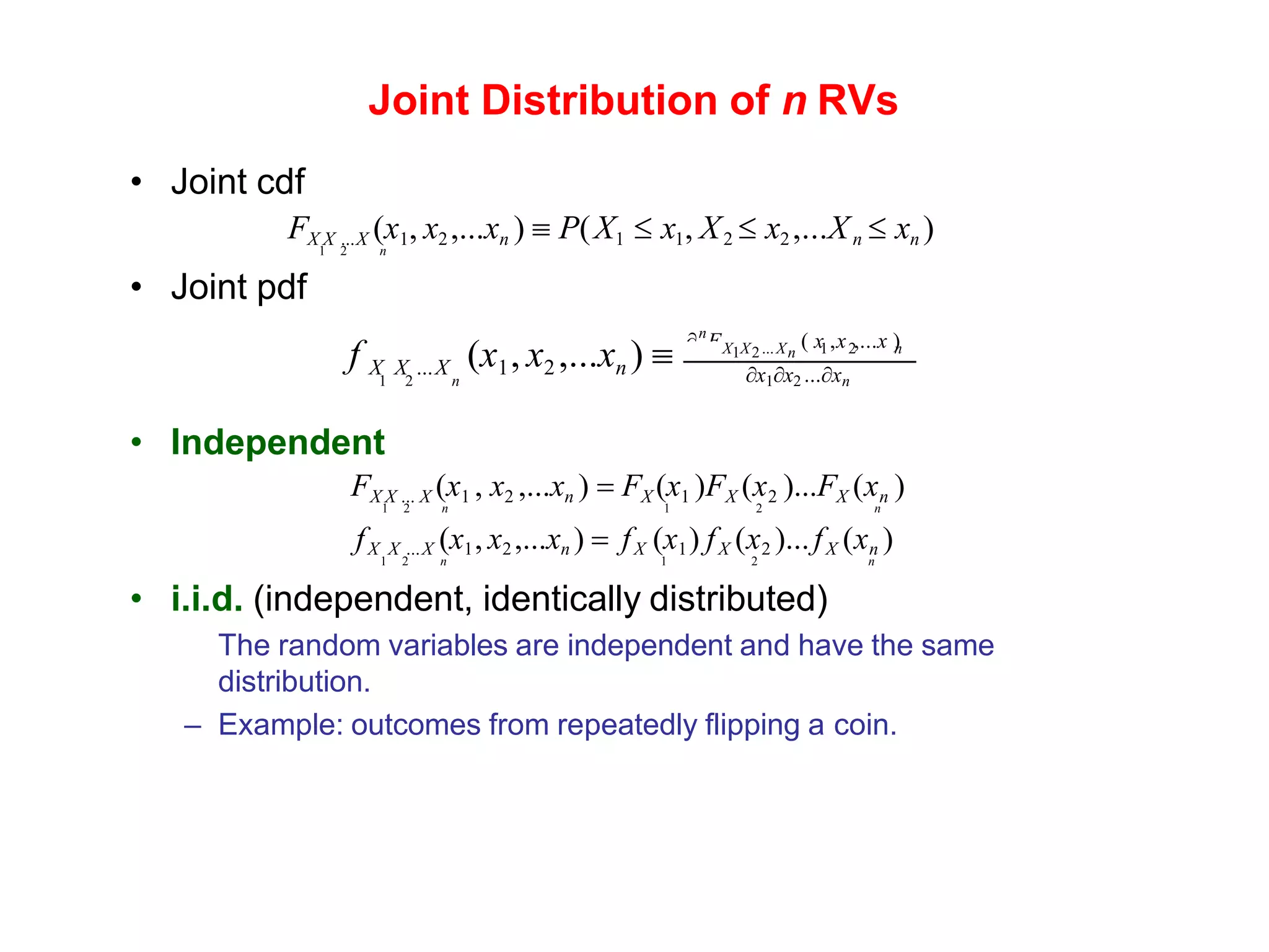
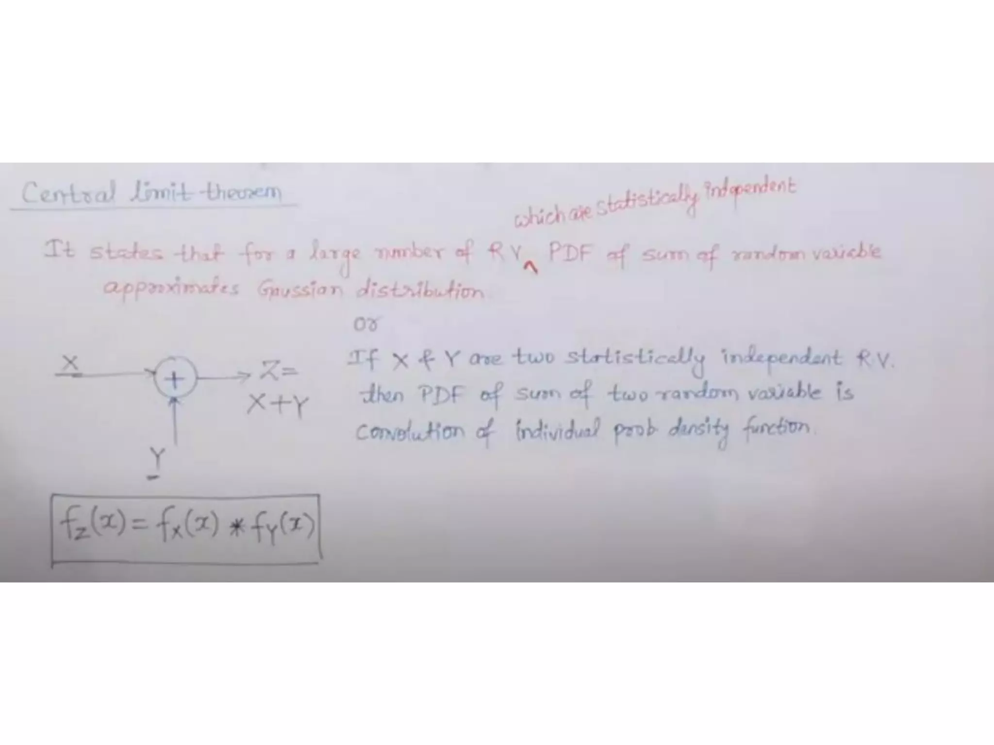
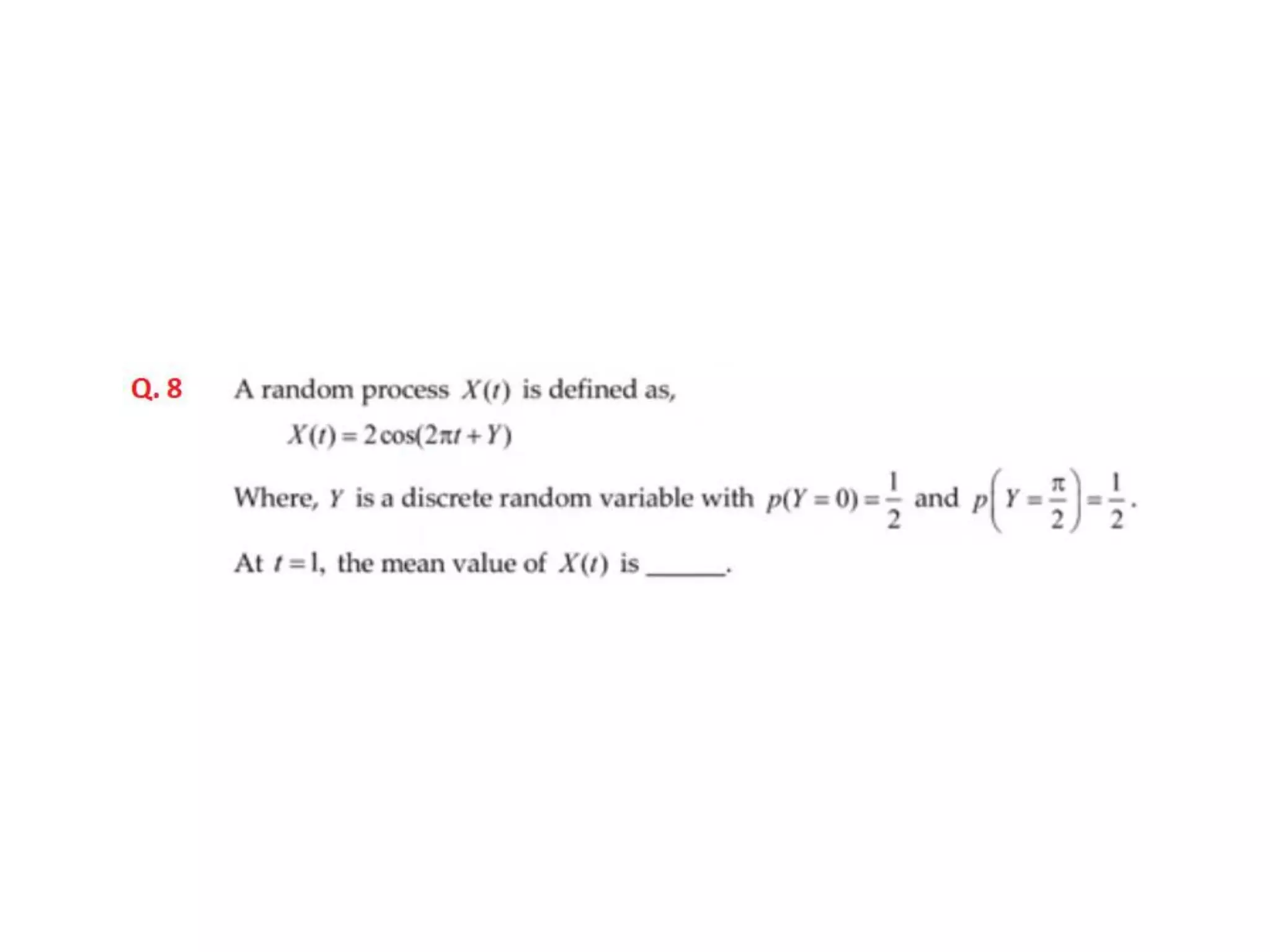
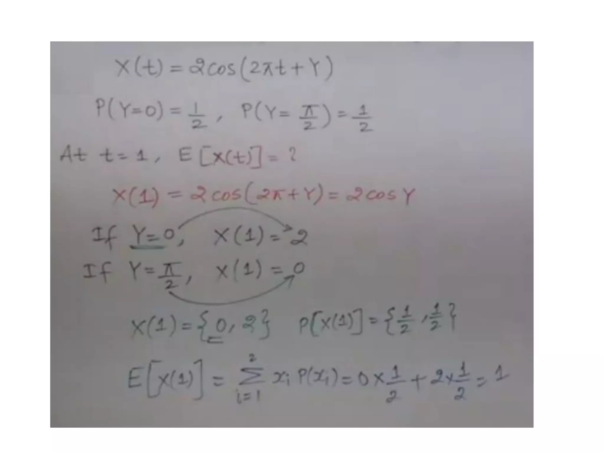
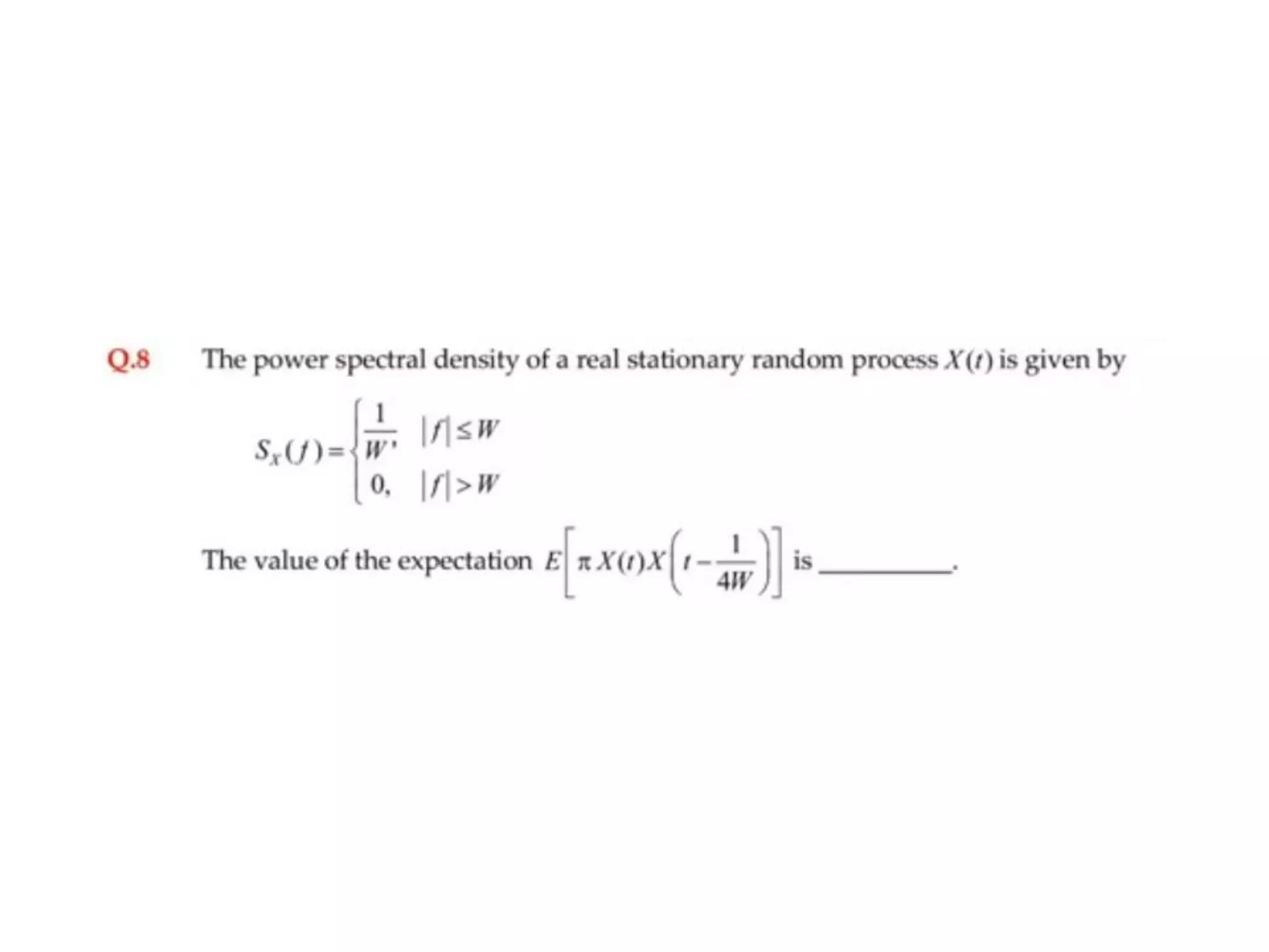
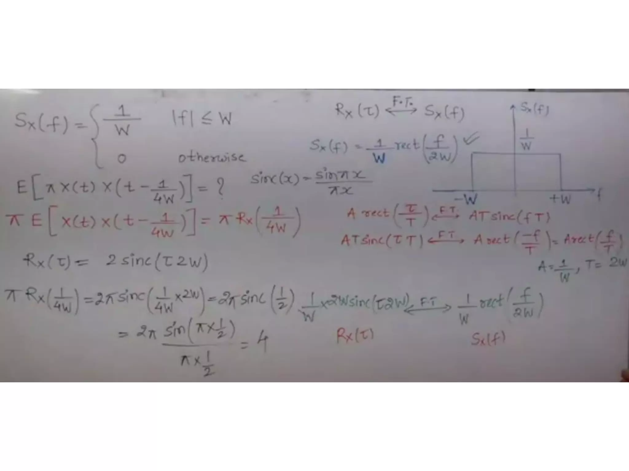
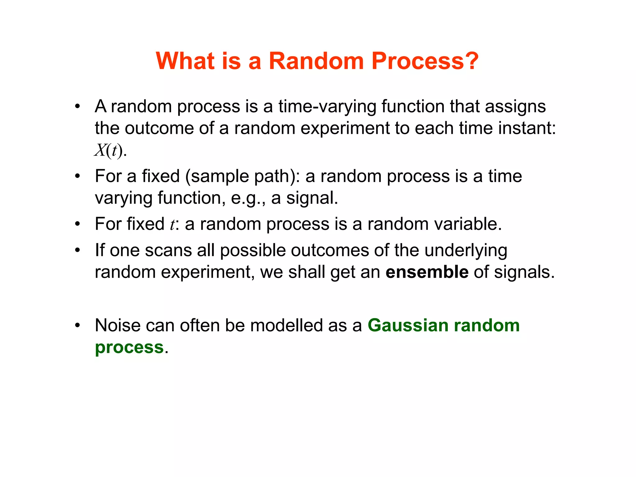
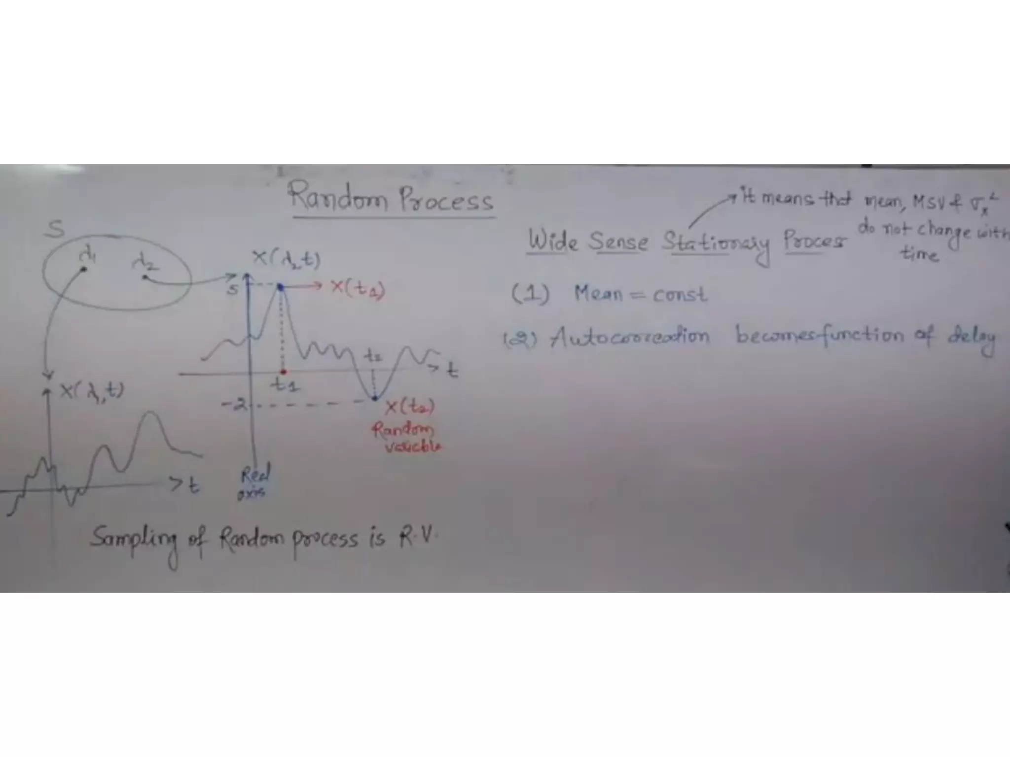
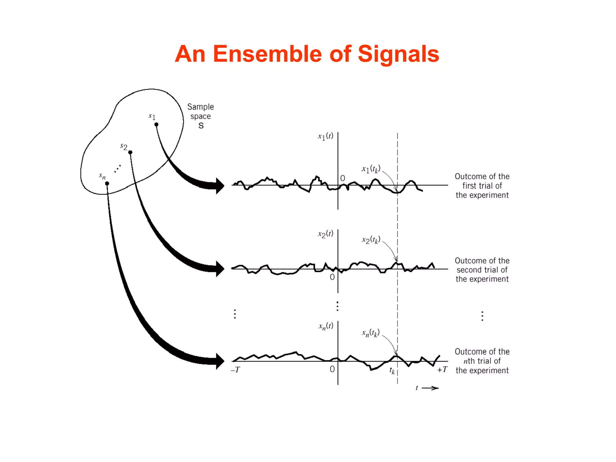
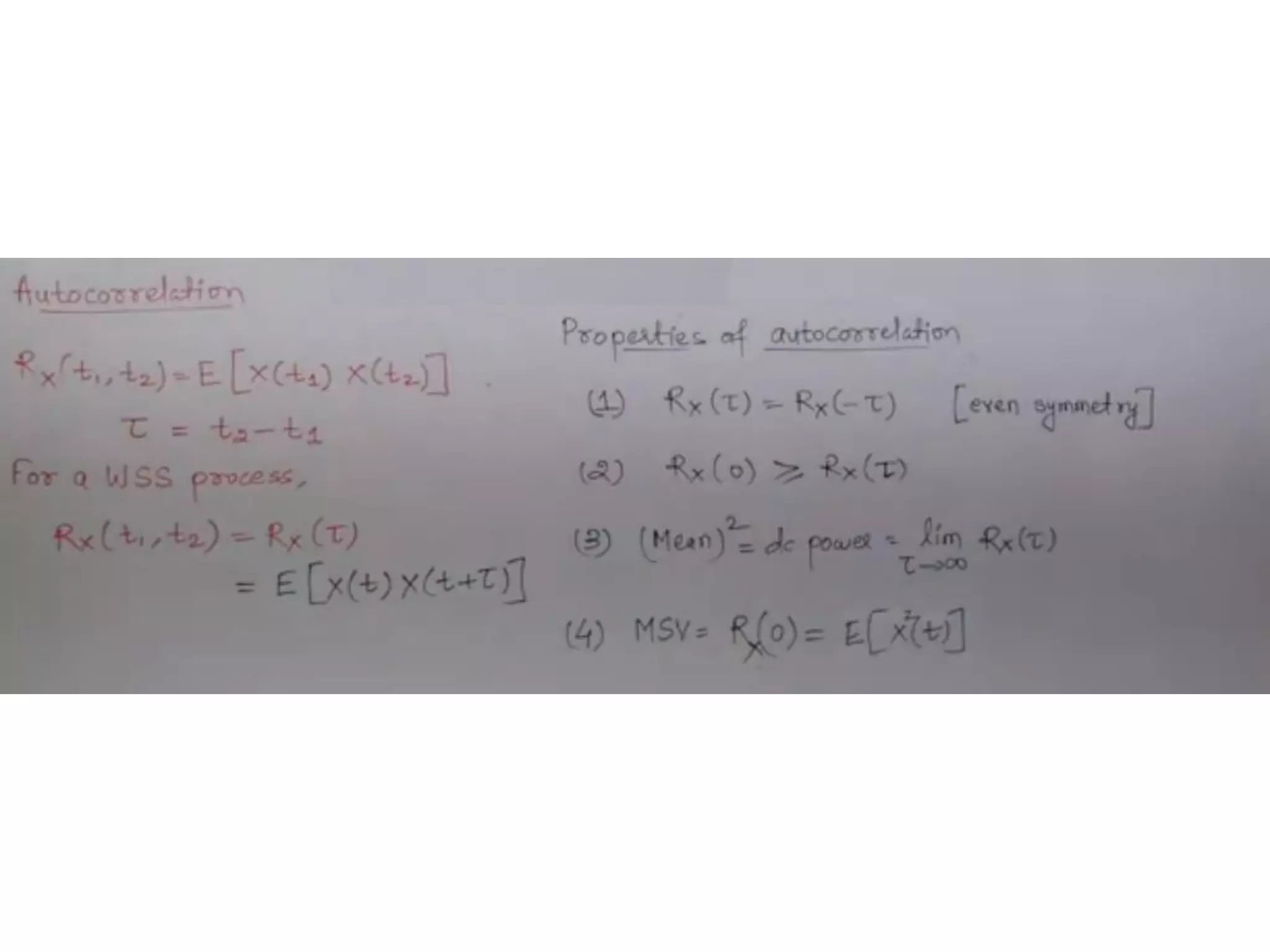
1) The document discusses key concepts in probability and random processes including random variables, probability density functions, mean and variance, joint distributions, and the central limit theorem. 2) It defines a random process as a time-varying function that assigns outcomes of a random experiment to time instances. Power spectral density measures the distribution of power over frequency for stationary random processes. 3) Random processes are widely used to model noise and interference in communication systems, which often exhibit random behavior. Probability and stochastic models provide important mathematical tools for analyzing communication systems.

1. Communication Systems
Probability and Random Processes
Dr. Irfan Arshad
Department of Electrical Engineering

2. Outline
• Probability
– How probability is defined
– cdf and pdf
– Mean and variance
Joint distribution
– Central limit theorem
• Random processes
– Definition
– Stationary random processes
– Power spectral density

3. Why Probability/Random Process?
• Probability is the core mathematical tool for communication
theory.
• The stochastic model is widely used in the study of
communication systems.
• Consider a radio communication system where the received
signal is a random process in nature:
– Message is random. No randomness, no information.
– Interference is random.
– Noise is a random process.
– And many more (delay, phase, fading, ...)
• Other real-world applications of probability and random
processes include
– Stock market modelling, gambling etc

4. Probabilistic Concepts
• What is a random variable (RV)?
– It is a variable that takes its values from the outputs of a random
experiment.
• What is a random experiment?
– It is an experiment the outcome of which cannot be predicted
precisely.
– All possible identifiable outcomes of a random experiment
constitute its sample space S.
– An event is a collection of possible outcomes of the random
experiment.
• Example
– For tossing a coin, S = { H, T }
– For rolling a die, S = { 1, 2, …, 6 }

6. Probability Properties
• PX(xi): the probability of the random variable X taking on
the value xi
• The probability of an event to happen is a non-negative
number, with the following properties:
– The probability of the event that includes all possible outcomes of
the experiment is 1.
– The probability of two events that do not have any common
outcome is the sum of the probabilities of the two events
separately.
• Example
– Roll a die: PX(x = k) = 1/6 for k = 1, 2, …, 6

7. Cumulative Distribution Function (CDF)
• The (cumulative) distribution function (cdf) of a random variable X
is defined as the probability of X taking a value less than the
argument x:
FX (x) = P( X x)
• Properties
FX (−) = 0, FX () =1
FX (x1 )  FX(x2 ) if x1x2

11. Probability Density Function (PDF)
• The probability density function (pdf) is defined as the derivative of
the cumulative distribution function:
dFX ( x )
X dx
f X ( y)dy
f (x) =
x
FX ( x) = 
a
f X ( y)dy
−
b
P (a  X  b ) = FX (b ) − FX (a ) = 
X X
dFX ( x )
dx
f (x) =  0 since F (x) is non - decreasing

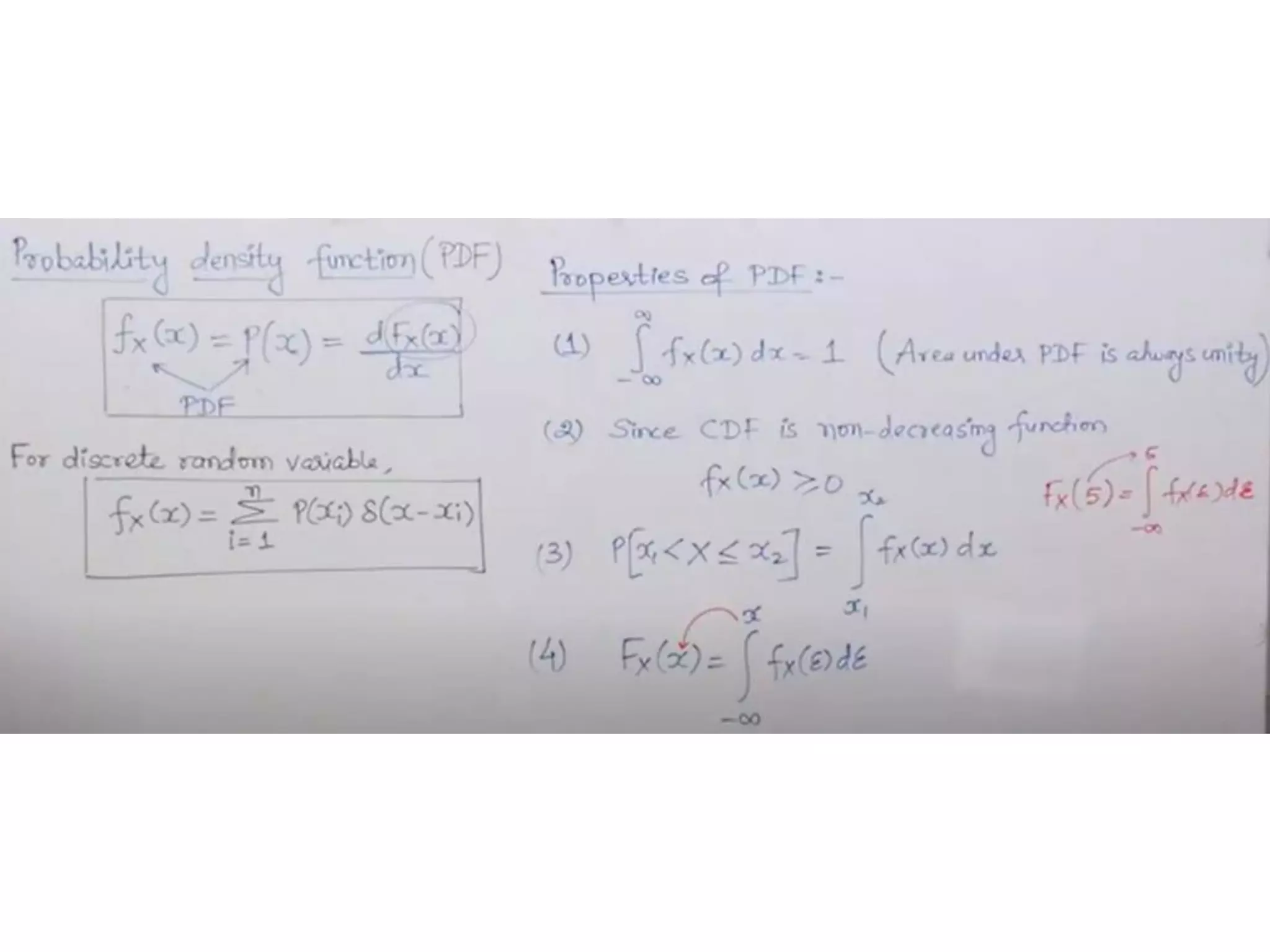
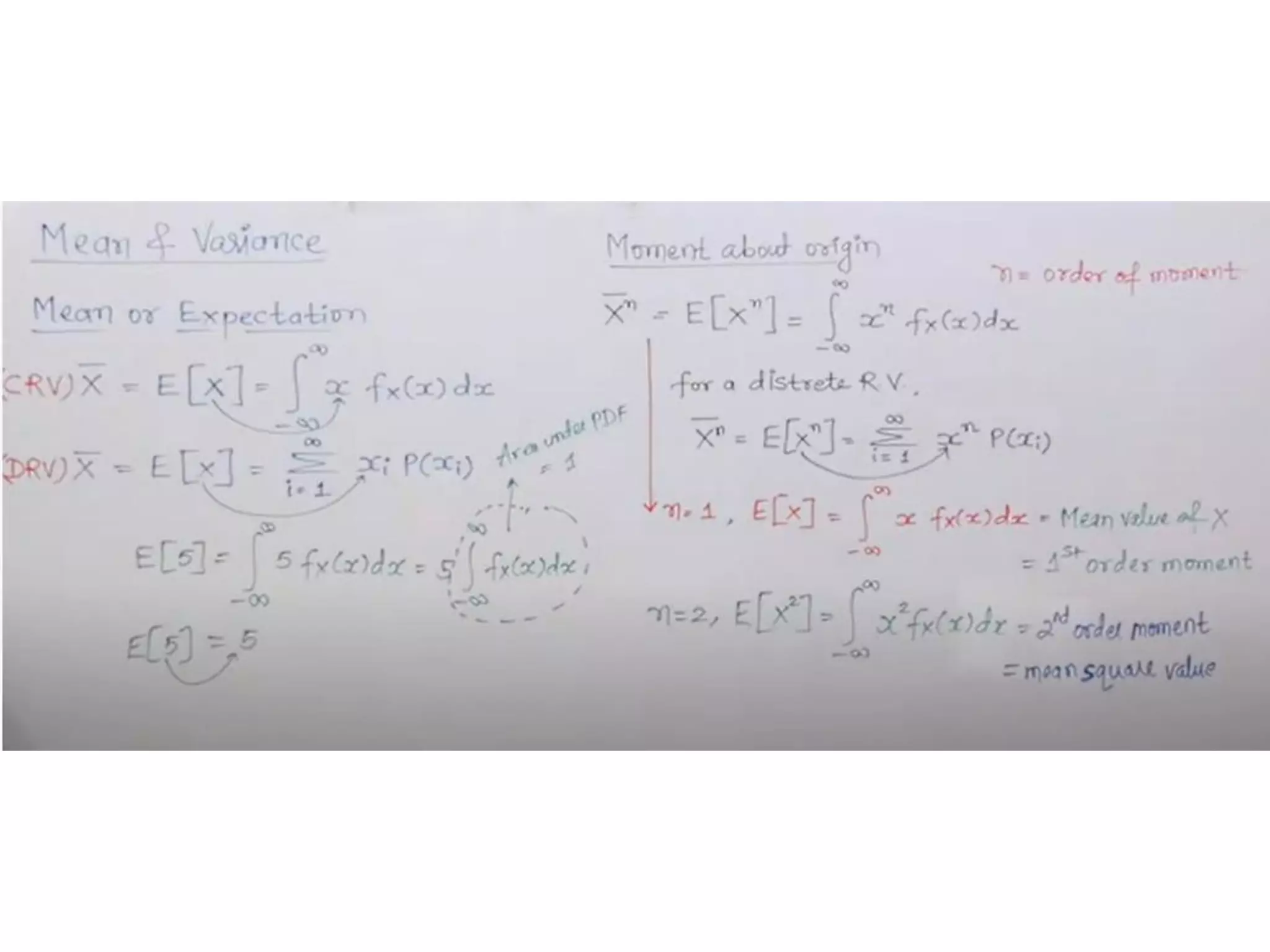
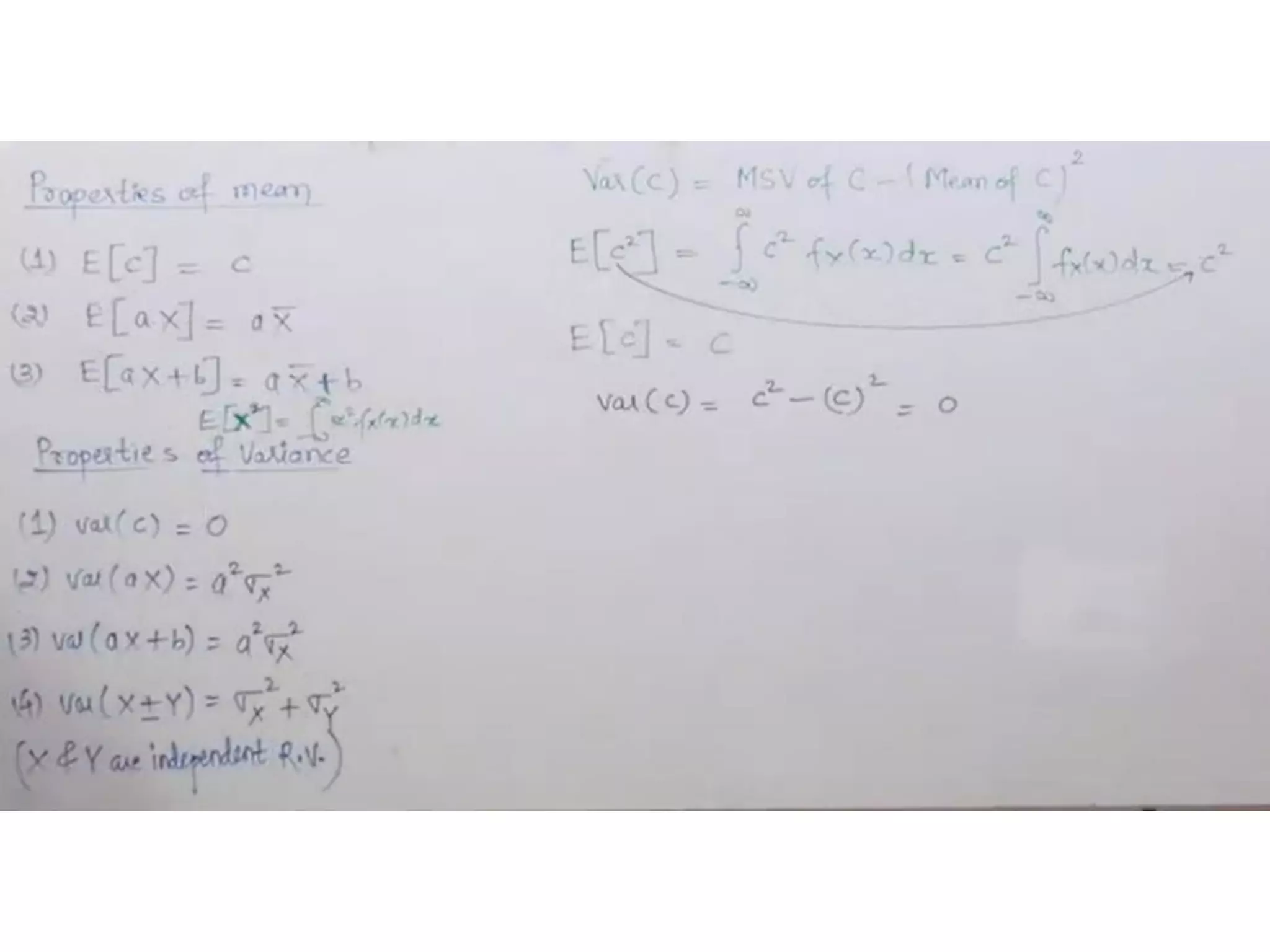
14. Mean and Variance
X X
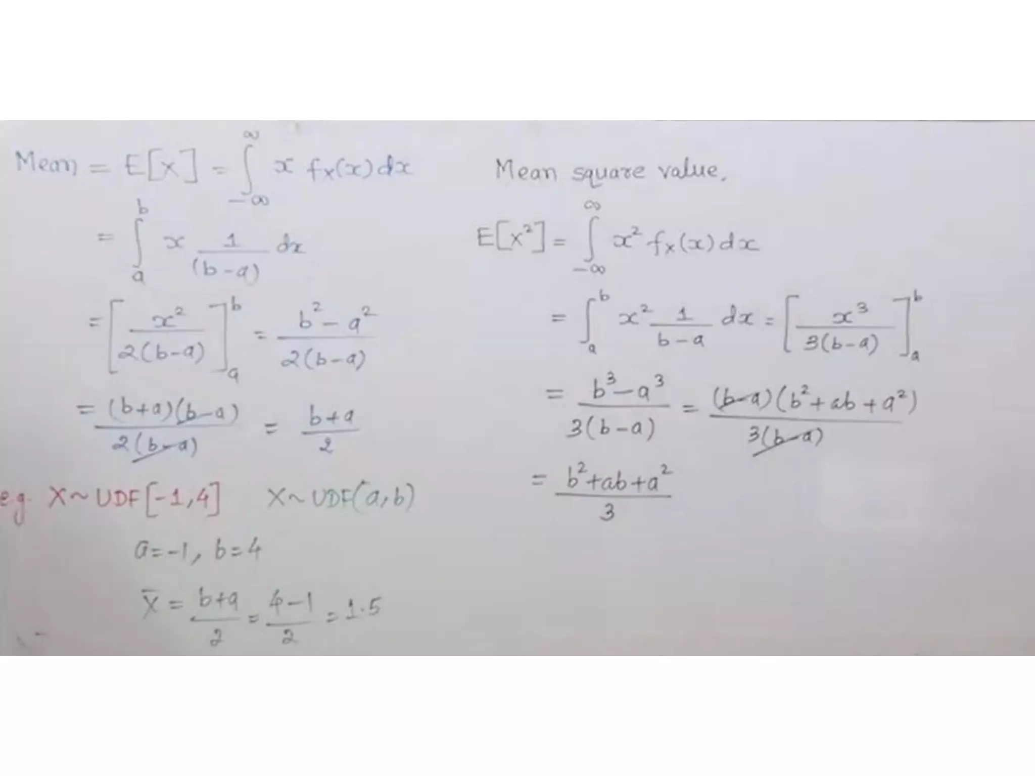
x f (x)dx
• Mean (or expected value  DC level):

E[X ] =  = 
E[ ]: expectation operator
−

18. 18
Normal (Gaussian) Distribution
The probability density function of a normal random variable is given by:
It looks like this:
Bell shaped, Symmetrical around the mean …
f X ( x)
x
0 m

19. Error Function

21. Gaussian Random Variable (GRV)

23. CDF of GRV

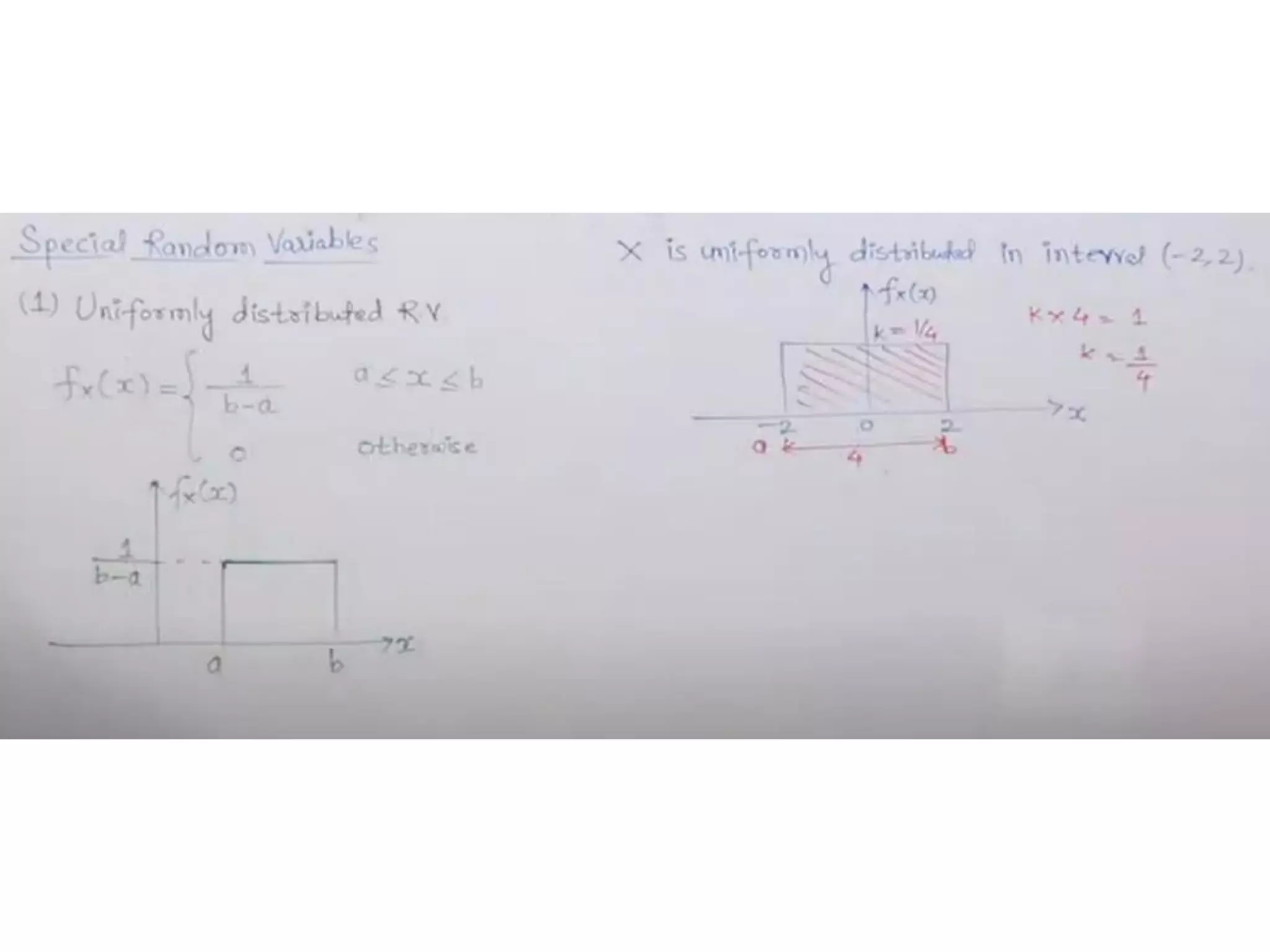
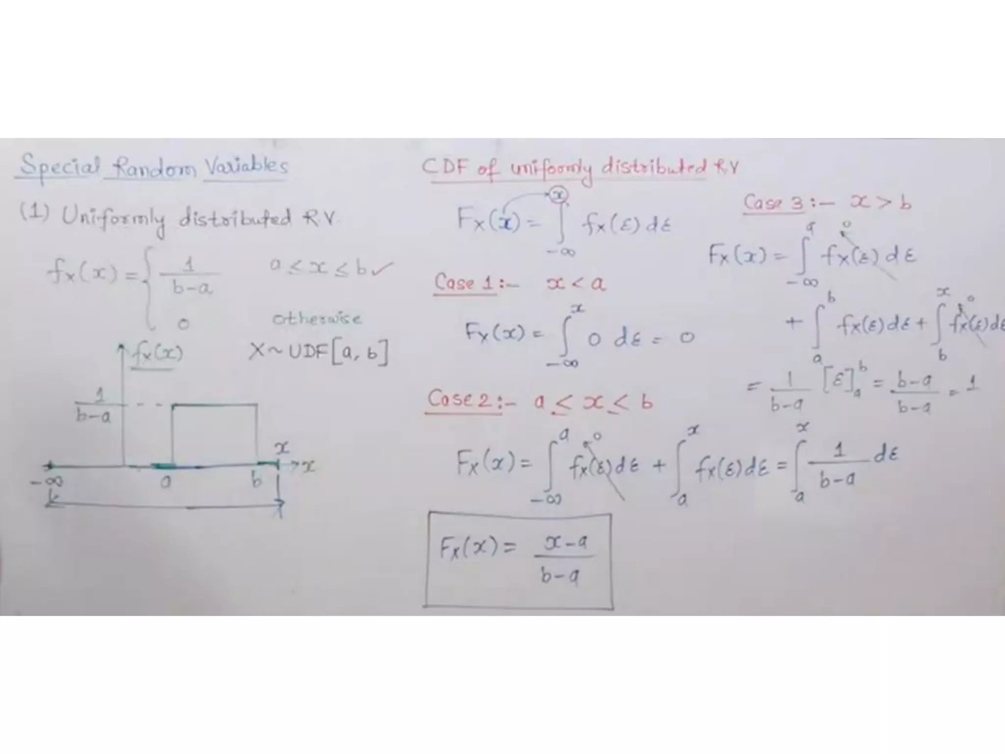
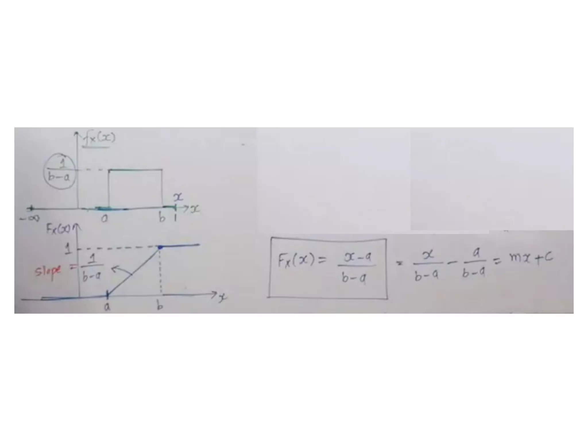
24. Uniform Distribution
fX(x)
1

X
a  x  b
f (x) = 
b − a

2
a + b
E [ X ]=
0
0
 x − a
FX ( x) = 
b −a
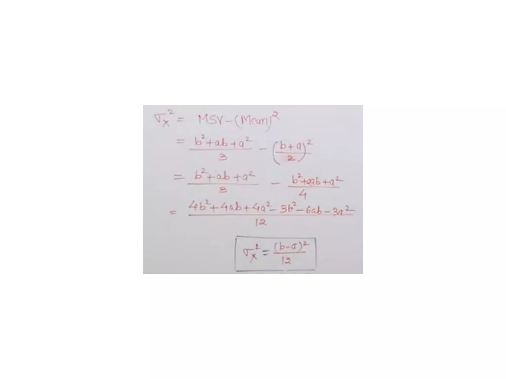
2
12
X

2
=
(b- a)
elsewhere
x  a
a  x  b
x  b

1

30. Joint Distribution
• Joint distribution function for two random variables X and Y
FXY (x, y) = P( X  x,Y  y)
• Joint probability density function
XY xy
2
FXY (x, y)
f (x, y) =
• Properties  
1) FXY (, ) =   f XY (u, v)dudv =1
− −
2) f X (x) = f XY (x,y)dy


3) fY (x) = f XY (x,y)dx
x=−
y=−


4) X , Y are independent  fXY (x, y) = fX (x) fY (y)
5) X , Y are uncorrelated  E[XY] = E[X ]E[Y]

31. Joint Distribution
• Joint distribution function for two random variables X and Y
FXY (x, y) = P( X  x,Y  y)
• Joint probability density function
XY xy
2
FXY (x, y)
f (x, y) =
• Properties  
1) FXY (, ) =   f XY (u, v)dudv =1
− −
2) f X (x) = f XY (x,y)dy


3) fY (x) = f XY (x,y)dx
x=−
y=−


4) X , Y are independent  fXY (x, y) = fX (x) fY (y)
5) X , Y are uncorrelated  E[XY] = E[X ]E[Y]

32. Joint Distribution of n RVs
• Joint cdf
FX X ...X (x1, x2 ,...xn )  P(X1  x1, X2  x2 ,...Xn  xn )
1 2 n
• Joint pdf
n
 F n
( x ,x ,...x )
x1x2 ...xn
X X ...X 1 2
1 2 n
f X X ...X (x1, x2 ,...xn ) 
1 2 n
• Independent
FX X ... X (x1 , x2 ,...xn ) = FX (x1 )FX (x2 )...FX (xn )
1 2 n 1 2 n
fX X ...X (x1, x2 ,...xn ) = fX (x1) fX (x2 )...fX (xn )
1 2 n 1 2 n
• i.i.d. (independent, identically distributed)
The random variables are independent and have the same
distribution.
– Example: outcomes from repeatedly flipping a coin.

33. Central Limit Theorem
x1 +x2
x1
“
”
x1 +x2
+ x3
x1 + x2+
x3 +x4
• For i.i.d. random variables,
z = x1 + x2 +· · ·+ xn
tends to Gaussian as n
goes to infinity.
• Extremely useful in
communications.
• That’s why noise is usually
Gaussian. We often say
Gaussian noise or
“Gaussian channel” in
communications.
Illustration of convergence to Gaussian
distribution

38. What is a Random Process?
• A random process is a time-varying function that assigns
the outcome of a random experiment to each time instant:
X(t).
• For a fixed (sample path): a random process is a time
varying function, e.g., a signal.
• For fixed t: a random process is a random variable.
• If one scans all possible outcomes of the underlying
random experiment, we shall get an ensemble of signals.
• Noise can often be modelled as a Gaussian random
process.

40. An Ensemble of Signals

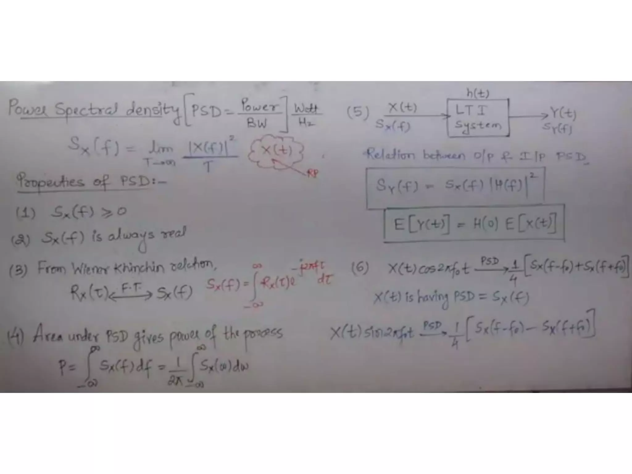
42. Power Spectral Density
• Power spectral density (PSD) is a function that measures
the distribution of power of a random process with
frequency.
• PSD is only defined for stationary processes.
• Wiener-Khinchine relation: The PSD is equal to the
Fourier transform of its autocorrelation function:

X
X
−
R ( )e− j 2 f
d
S ( f ) =
– A similar relation exists for deterministic signals
• Then the average power can be found as
X X

S ( f )df
−
P = E[ X 2
(t)]= R (0) = 
• The frequency content of a process depends on how
rapidly the amplitude changes as a function of time.
– This can be measured by the autocorrelation function.

44. Passing Through a Linear System
• Let Y(t) obtained by passing random process X(t) through
a linear system of transfer function H(f). Then the PSD of
Y(t) 2
SY ( f ) = H (f ) SX ( f ) (2.1)
• If X(t) is a Gaussian process, then Y(t) is also a Gaussian
process.
– Gaussian processes are very important in communications.