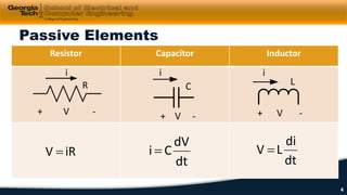
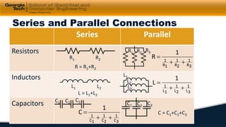
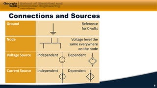
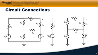
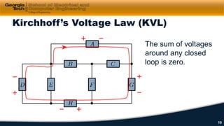
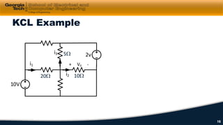
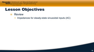
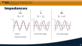
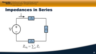
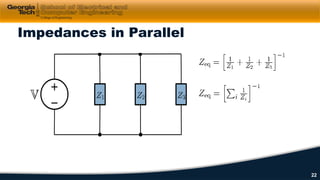
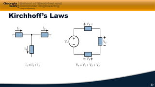
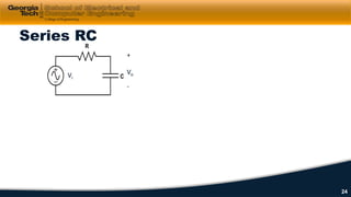
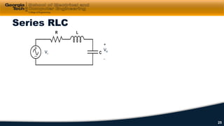
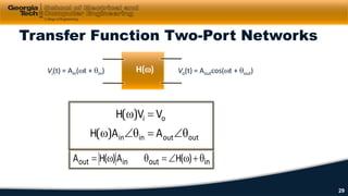
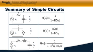
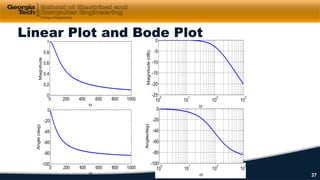
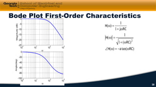
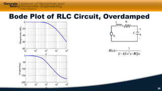
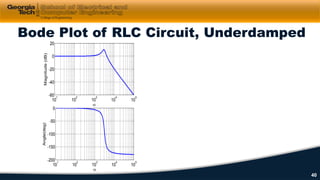
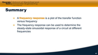
School of Electrical and Computer Engineering
Introduction to Electronics
Module 1: Overview and
Background
An introduction to electronic components and a study of circuits
containing such devices.
Dr. Bonnie H. Ferri
Professor and Associate Chair
School of Electrical and
Computer Engineering
School of Electrical and Computer Engineering
Review of Circuit
Elements
Review linear circuit components and properties
 Review
 Resistors, capacitors, inductors
○ i-v characteristics of these elements
 Sources, nodes
Lesson Objectives
3
Passive Elements
Resistor Capacitor Inductor
+ V -
i
R
iRV =
+ V -
C
i
dt
dV
Ci =
+ V -
L
i
dt
di
LV =
4
Series and Parallel Connections
Series Parallel
Resistors
Inductors
Capacitors
R1 R2
R = R1+R2
R1 R2
R3
3R
1
2R
1
1R
1
1
R
++
=
3C
1
2C
1
1C
1
1
C
++
=
C1 C2
C3
C1 C2 C3
C = C1+C2+C3
3L
1
2L
1
1L
1
1
L
++
=
L = L1+L2
L1 L2
L1
L2
L3
Connections and Sources
Ground Reference
for 0 volts
Node Voltage level the
same everywhere
on the node
Voltage Source Independent Dependent
Current Source Independent Dependent
+
-
6
Circuit Connections
V1
R1
R2
R3
R4
R5
+
V0
-
R6
IS V1
R1
R2
R3
R4
R5
+
V0
-
R6
IS
7
Dr. Bonnie H. Ferri
Professor and Associate Chair
School of Electrical and
Computer Engineering
School of Electrical and Computer Engineering
Review of
Kirchoff’s Laws
Review of KVL and KCL
 Review
 Kirchhoff’s Current Law (KCL)
 Kirchhoff’s Voltage Law (KVL)
Lesson Objectives
9
Kirchhoff’s Voltage Law (KVL)
The sum of voltages
around any closed
loop is zero.
10
KVL Quiz
+
2v
-
+
4v
-
- 5v ++ -1v -
- VH +
11
KVL and Parallel Circuits
12
KVL Example
10V
2v
+ V0 -i1
i2
i3
20Ω 10Ω
5Ω
13
Kirchhoff’s Current Law (KCL)
∑ ∑= leavingentering ii
14
KCL and Series Circuits
15
KCL Example
10V
2v
+ V0 -i1
i2
i3
20Ω 10Ω
5Ω
16
 Introduced KVL and KCL
 Applied KVL to parallel elements
 Applied KCL to series elements
 Solved a simple circuit using
Kirchhoff’s Laws
Summary
17
Dr. Bonnie H. Ferri
Professor and Associate Chair
School of Electrical and
Computer Engineering
School of Electrical and Computer Engineering
Review of
Impedance
Review of Impedance for Analyzing AC Circuits
 Review
 Impedances for steady-state sinusoidal inputs (AC)
Lesson Objectives
19
Impedances
In-phase Current leads voltage Current lags voltage
Frequency invariant
20
Impedances in Series
21
Impedances in Parallel
22
Kirchhoff’s Laws
23
Series RC
+
Vo
-
Vi
24
Series RLC
Vi
+
Vo
-
25
 Introduced KVL and KCL
 Applied KVL to parallel elements
 Applied KCL to series elements
 Solved a simple circuit using
Kirchhoff’s Laws
Summary
26
Dr. Bonnie H. Ferri
Professor and Associate Chair
School of Electrical and
Computer Engineering
School of Electrical and Computer Engineering
Review of
Transfer Functions
Review of transfer functions for characterizing circuits
 Review transfer functions
 To characterize a circuit
 To find frequency response curves
Lesson Objectives
28
Transfer Function Two-Port Networks
Vi(t) = Ain(ωt + θin) H(ω) Vo(t) = Aoutcos(ωt + θout)
inoutinout )(HA)(HA θ+ω∠=θω=
outoutinin
oi
AAH
VVH
θ∠=θ∠ω
=ω
)(
)(
29
Summary of Simple Circuits
jRC1
1
H
ω+
=ω)(
+
Vo
-Vi
+
Vo
-
Vi
+
Vo
-
Vi jRCLC1
1
H 2
ω+ω−
=ω)(
jRC1
jRC
H
ω+
ω
=ω)(
30
 Defined transfer function for Two-Port
Networks
 Showed transfer functions of simple circuits
Summary
31
Dr. Bonnie H. Ferri
Professor and Associate Chair
School of Electrical and
Computer Engineering
School of Electrical and Computer Engineering
Review of Frequency
Response Plots
(Bode)
Review of linear plots and Bode plots to show the frequency
characteristics of signals and circuits
 Define the frequency response for a transfer function
 Show linear plots and Bode plots
Lesson Objectives
)(ωH
Magnitude Plot: |H(ω)| vs ω
Angle Plot: ∠H(ω) vs ω
33
Frequency Response
0 200 400 600 800 1000
0
0.2
0.4
0.6
0.8
1
ω
Magnitude
0 200 400 600 800 1000
-100
-80
-60
-40
-20
0
ωAngle(deg)
Transfer Function
)tan()(
)(
)(
)(
ω−=ω∠
ω+
=ω
ω+
=ω
RCaH
RC1
1
H
jRC1
1
H
2
+
Vo
-
Vi
34
Circuit Response
Vi
Vo
0 0.05 0.1 0.15 0.2 0.25
-2
-1
0
1
2
Time (sec)
v(t)
0 0.05 0.1 0.15 0.2 0.25
-1.5
-1
-0.5
0
0.5
1
1.5
Time (sec)
v(t)
0 200 400 600 800 1000
0
0.2
0.4
0.6
0.8
1
ω
Magnitude
Vi = cos(50t) + cos(800t) Vo = 0.95cos(50t-20o) + 0.13cos(800t-85o)
0 200 400 600 800 1000
-100
-80
-60
-40
-20
0
ω
Angle(deg)
35
Bode Plots
Frequency ω (rad/sec) or f (Hz)1 10 100 1000
36
Linear Plot and Bode Plot
10
0
10
1
10
2
10
3
-100
-80
-60
-40
-20
0
ω
Angle(deg)
10
0
10
1
10
2
10
3
-25
-20
-15
-10
-5
0
ω
Magnitude(dB)
0 200 400 600 800 1000
-100
-80
-60
-40
-20
0
ω
Angle(deg)
0 200 400 600 800 1000
0
0.2
0.4
0.6
0.8
1
ω
Magnitude
37
Bode Plot First-Order Characteristics
10
0
10
1
10
2
10
3
-100
-80
-60
-40
-20
0
ω
Angle(deg)
10
0
10
1
10
2
10
3
-25
-20
-15
-10
-5
0
ω
Magnitude(dB)
)tan()(
)(1
1
)(
1
1
)(
2
RCaH
RC
H
RCj
H
ω−=ω∠
ω+
=ω
ω+
=ω
38
Bode Plot of RLC Circuit, Overdamped
10
1
10
2
10
3
10
4
10
5
-80
-60
-40
-20
0
ω
Magnitude(dB)
10
1
10
2
10
3
10
4
10
5
-200
-150
-100
-50
0
ω
Angle(deg)
vs
+
-
vc
C
L
vs
+
-
-
R
ω+ω−
=ω
RCjLC
H
)(
)( 2
1
1
39
Bode Plot of RLC Circuit, Underdamped
10
1
10
2
10
3
10
4
10
5
-60
-40
-20
0
20
ω
Magnitude(dB)
10
1
10
2
10
3
10
4
10
5
-200
-150
-100
-50
0
ω
Angle(deg)
40
 A is a plot of the transfer function
versus frequency
 The frequency response can be used to determine the
steady-state sinusoidal response of a circuit at different
frequencies
Summary
41

Module 1 ELECTRONICS

  • 1.
    School of Electricaland Computer Engineering Introduction to Electronics Module 1: Overview and Background An introduction to electronic components and a study of circuits containing such devices.
  • 2.
    Dr. Bonnie H.Ferri Professor and Associate Chair School of Electrical and Computer Engineering School of Electrical and Computer Engineering Review of Circuit Elements Review linear circuit components and properties
  • 3.
     Review  Resistors,capacitors, inductors ○ i-v characteristics of these elements  Sources, nodes Lesson Objectives 3
  • 4.
    Passive Elements Resistor CapacitorInductor + V - i R iRV = + V - C i dt dV Ci = + V - L i dt di LV = 4
  • 5.
    Series and ParallelConnections Series Parallel Resistors Inductors Capacitors R1 R2 R = R1+R2 R1 R2 R3 3R 1 2R 1 1R 1 1 R ++ = 3C 1 2C 1 1C 1 1 C ++ = C1 C2 C3 C1 C2 C3 C = C1+C2+C3 3L 1 2L 1 1L 1 1 L ++ = L = L1+L2 L1 L2 L1 L2 L3
  • 6.
    Connections and Sources GroundReference for 0 volts Node Voltage level the same everywhere on the node Voltage Source Independent Dependent Current Source Independent Dependent + - 6
  • 7.
  • 8.
    Dr. Bonnie H.Ferri Professor and Associate Chair School of Electrical and Computer Engineering School of Electrical and Computer Engineering Review of Kirchoff’s Laws Review of KVL and KCL
  • 9.
     Review  Kirchhoff’sCurrent Law (KCL)  Kirchhoff’s Voltage Law (KVL) Lesson Objectives 9
  • 10.
    Kirchhoff’s Voltage Law(KVL) The sum of voltages around any closed loop is zero. 10
  • 11.
    KVL Quiz + 2v - + 4v - - 5v++ -1v - - VH + 11
  • 12.
    KVL and ParallelCircuits 12
  • 13.
    KVL Example 10V 2v + V0-i1 i2 i3 20Ω 10Ω 5Ω 13
  • 14.
    Kirchhoff’s Current Law(KCL) ∑ ∑= leavingentering ii 14
  • 15.
    KCL and SeriesCircuits 15
  • 16.
    KCL Example 10V 2v + V0-i1 i2 i3 20Ω 10Ω 5Ω 16
  • 17.
     Introduced KVLand KCL  Applied KVL to parallel elements  Applied KCL to series elements  Solved a simple circuit using Kirchhoff’s Laws Summary 17
  • 18.
    Dr. Bonnie H.Ferri Professor and Associate Chair School of Electrical and Computer Engineering School of Electrical and Computer Engineering Review of Impedance Review of Impedance for Analyzing AC Circuits
  • 19.
     Review  Impedancesfor steady-state sinusoidal inputs (AC) Lesson Objectives 19
  • 20.
    Impedances In-phase Current leadsvoltage Current lags voltage Frequency invariant 20
  • 21.
  • 22.
  • 23.
  • 24.
  • 25.
  • 26.
     Introduced KVLand KCL  Applied KVL to parallel elements  Applied KCL to series elements  Solved a simple circuit using Kirchhoff’s Laws Summary 26
  • 27.
    Dr. Bonnie H.Ferri Professor and Associate Chair School of Electrical and Computer Engineering School of Electrical and Computer Engineering Review of Transfer Functions Review of transfer functions for characterizing circuits
  • 28.
     Review transferfunctions  To characterize a circuit  To find frequency response curves Lesson Objectives 28
  • 29.
    Transfer Function Two-PortNetworks Vi(t) = Ain(ωt + θin) H(ω) Vo(t) = Aoutcos(ωt + θout) inoutinout )(HA)(HA θ+ω∠=θω= outoutinin oi AAH VVH θ∠=θ∠ω =ω )( )( 29
  • 30.
    Summary of SimpleCircuits jRC1 1 H ω+ =ω)( + Vo -Vi + Vo - Vi + Vo - Vi jRCLC1 1 H 2 ω+ω− =ω)( jRC1 jRC H ω+ ω =ω)( 30
  • 31.
     Defined transferfunction for Two-Port Networks  Showed transfer functions of simple circuits Summary 31
  • 32.
    Dr. Bonnie H.Ferri Professor and Associate Chair School of Electrical and Computer Engineering School of Electrical and Computer Engineering Review of Frequency Response Plots (Bode) Review of linear plots and Bode plots to show the frequency characteristics of signals and circuits
  • 33.
     Define thefrequency response for a transfer function  Show linear plots and Bode plots Lesson Objectives )(ωH Magnitude Plot: |H(ω)| vs ω Angle Plot: ∠H(ω) vs ω 33
  • 34.
    Frequency Response 0 200400 600 800 1000 0 0.2 0.4 0.6 0.8 1 ω Magnitude 0 200 400 600 800 1000 -100 -80 -60 -40 -20 0 ωAngle(deg) Transfer Function )tan()( )( )( )( ω−=ω∠ ω+ =ω ω+ =ω RCaH RC1 1 H jRC1 1 H 2 + Vo - Vi 34
  • 35.
    Circuit Response Vi Vo 0 0.050.1 0.15 0.2 0.25 -2 -1 0 1 2 Time (sec) v(t) 0 0.05 0.1 0.15 0.2 0.25 -1.5 -1 -0.5 0 0.5 1 1.5 Time (sec) v(t) 0 200 400 600 800 1000 0 0.2 0.4 0.6 0.8 1 ω Magnitude Vi = cos(50t) + cos(800t) Vo = 0.95cos(50t-20o) + 0.13cos(800t-85o) 0 200 400 600 800 1000 -100 -80 -60 -40 -20 0 ω Angle(deg) 35
  • 36.
    Bode Plots Frequency ω(rad/sec) or f (Hz)1 10 100 1000 Frequency ω (rad/sec) or f (Hz)1 10 100 1000 36
  • 37.
    Linear Plot andBode Plot 10 0 10 1 10 2 10 3 -100 -80 -60 -40 -20 0 ω Angle(deg) 10 0 10 1 10 2 10 3 -25 -20 -15 -10 -5 0 ω Magnitude(dB) 0 200 400 600 800 1000 -100 -80 -60 -40 -20 0 ω Angle(deg) 0 200 400 600 800 1000 0 0.2 0.4 0.6 0.8 1 ω Magnitude 37
  • 38.
    Bode Plot First-OrderCharacteristics 10 0 10 1 10 2 10 3 -100 -80 -60 -40 -20 0 ω Angle(deg) 10 0 10 1 10 2 10 3 -25 -20 -15 -10 -5 0 ω Magnitude(dB) )tan()( )(1 1 )( 1 1 )( 2 RCaH RC H RCj H ω−=ω∠ ω+ =ω ω+ =ω 38
  • 39.
    Bode Plot ofRLC Circuit, Overdamped 10 1 10 2 10 3 10 4 10 5 -80 -60 -40 -20 0 ω Magnitude(dB) 10 1 10 2 10 3 10 4 10 5 -200 -150 -100 -50 0 ω Angle(deg) vs + - vc C L vs + - - R ω+ω− =ω RCjLC H )( )( 2 1 1 39
  • 40.
    Bode Plot ofRLC Circuit, Underdamped 10 1 10 2 10 3 10 4 10 5 -60 -40 -20 0 20 ω Magnitude(dB) 10 1 10 2 10 3 10 4 10 5 -200 -150 -100 -50 0 ω Angle(deg) 40
  • 41.
     A isa plot of the transfer function versus frequency  The frequency response can be used to determine the steady-state sinusoidal response of a circuit at different frequencies Summary 41