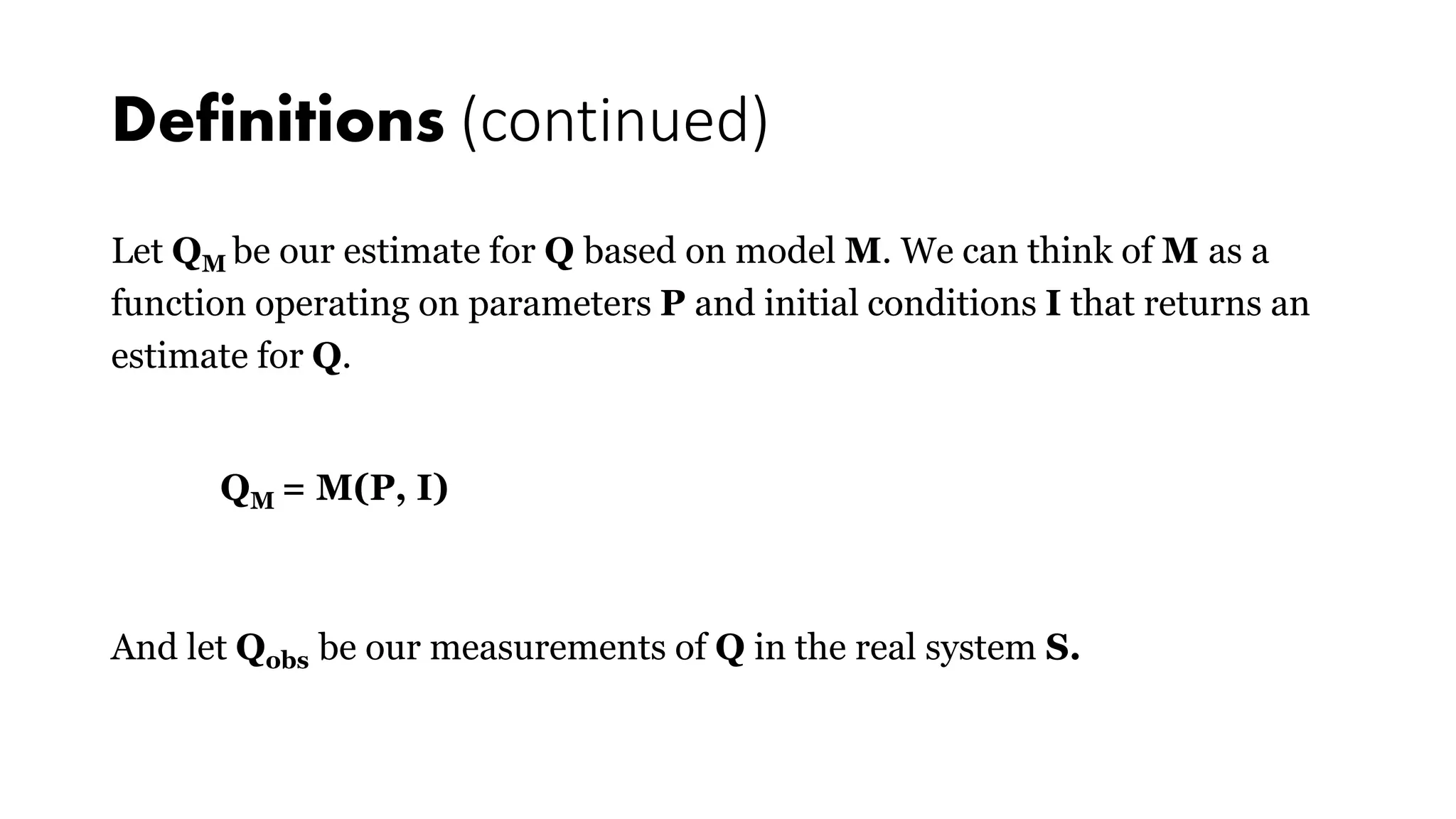
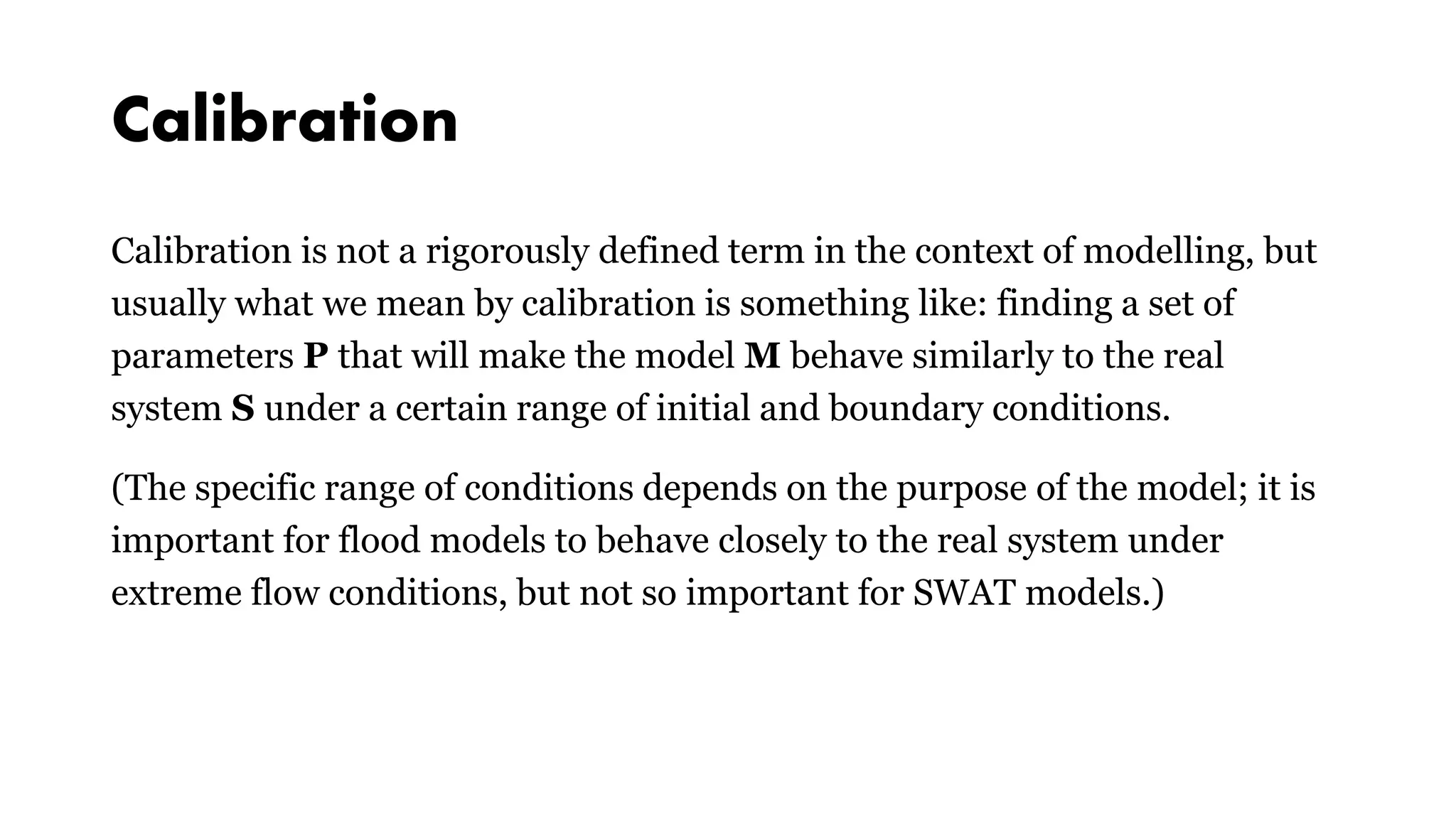
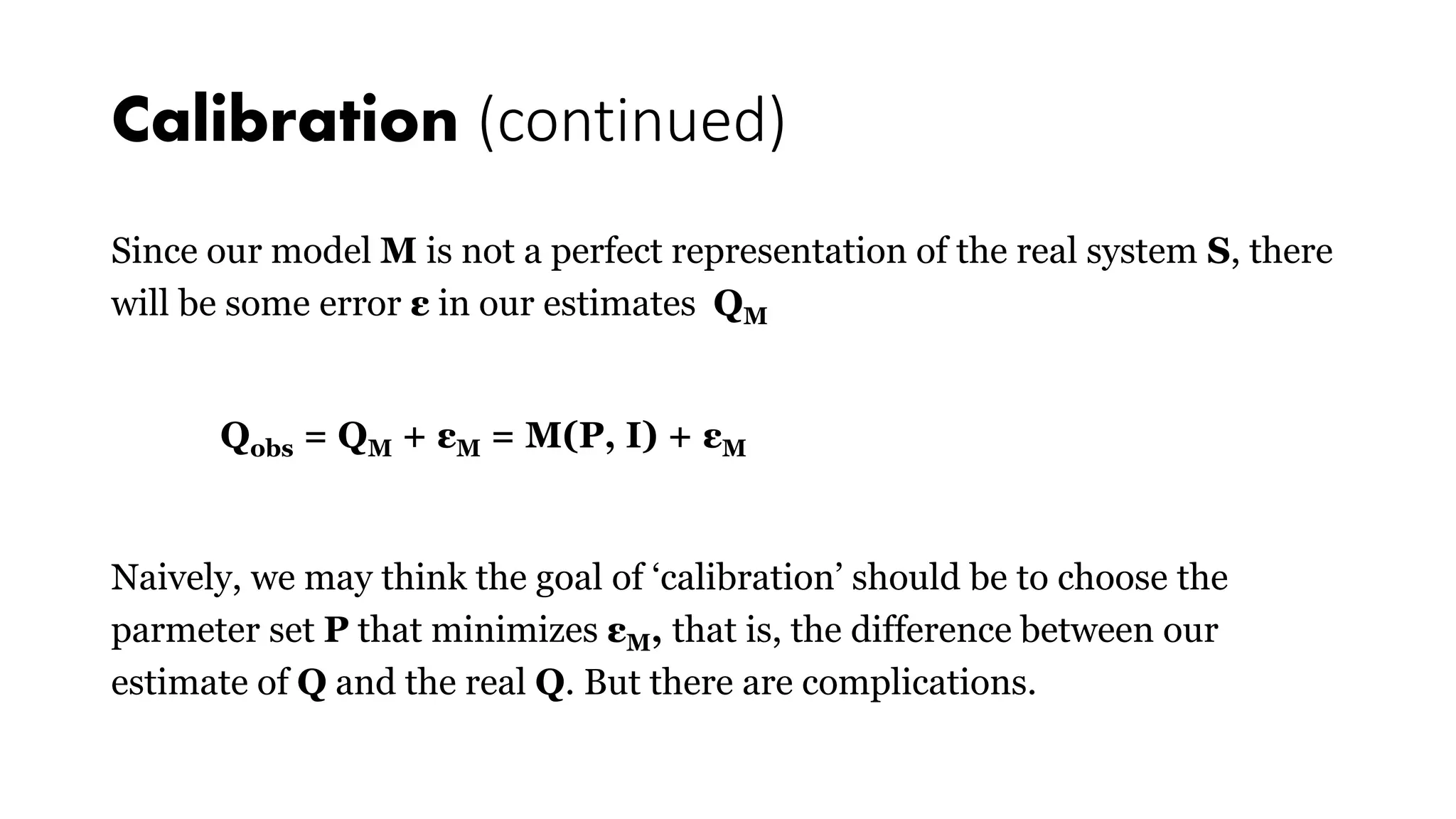
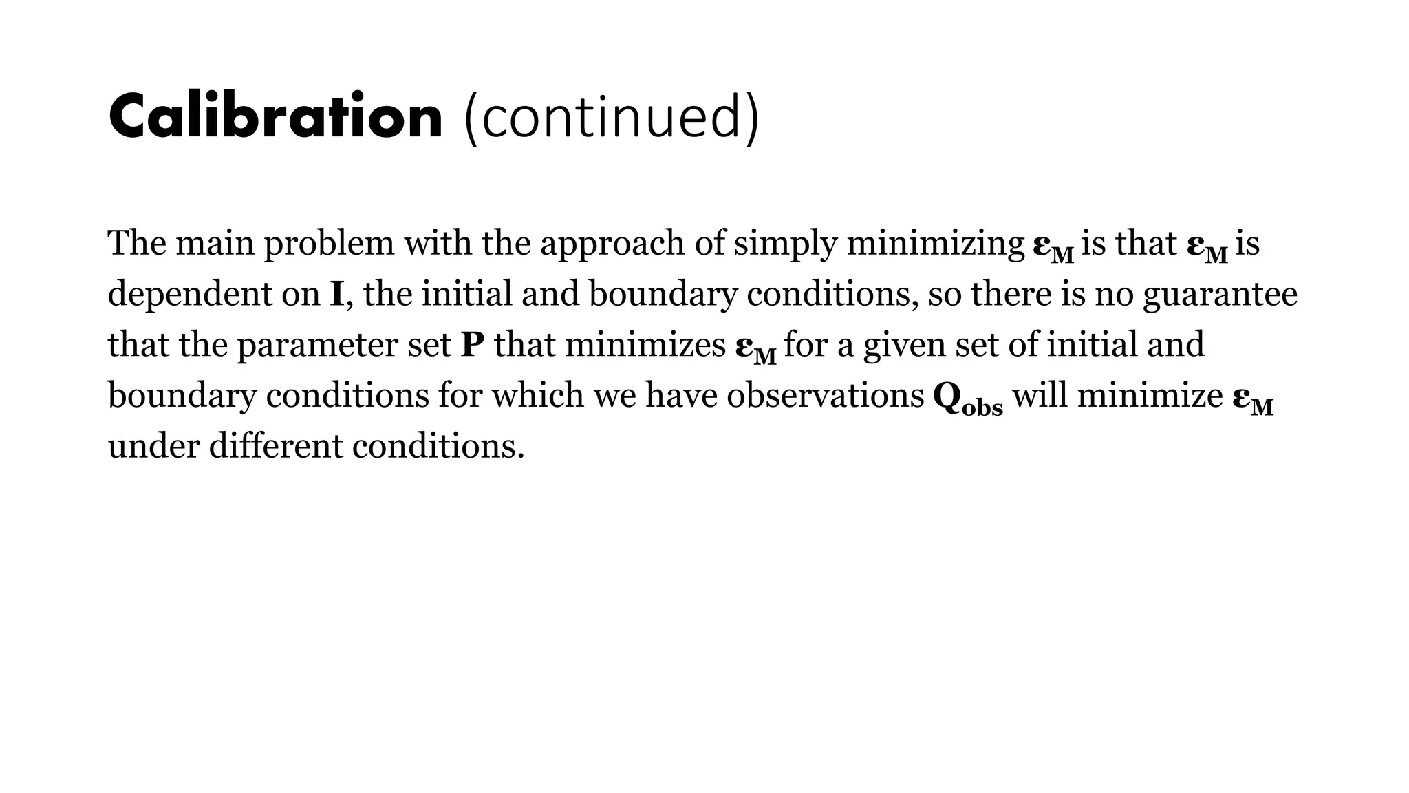
SlideShare a Scribd company logo
Calibration, Validation, and Uncertainty
In Environmental and Hydrological
Modeling
A Somewhat Bayesian Perspective
Outline
1. Definitions
2. Calibration
3. Validation
4. Uncertainty Analysis
Definitions
Let’s say we want to model the real system S (for example, a watershed), so
that we can estimate Q, (for example, streamflow, or water quality).
We have a model M meant to simulate the behavior of system S, based on
our knowledge of the processes involved (their causal structure, the
mathematical relationships between variables, etc.).
The model M has a number of parameters :
ρ1, ρ2, ρ3, ..., ρn
Let Φ be the set of parameters {ρ1, ρ2, ρ3, ..., ρn}.
Definitions (continued)
When we run the model we set the parameters to particular values:
ρ1 = p1, ρ2 = p2, ..., ρn = pn
Let P be the set of particular parameter values we use, {p1, p2, ..., pn}, such
that when we run the model we set
Φ = P
The model also depends on initial and boundary conditions Θ, which we set
to I.
Definitions (continued)
Let QM be our estimate for Q based on model M. We can think of M as a
function operating on parameters P and initial conditions I that returns an
estimate for Q.
QM = M(P, I)
And let Qobs be our measurements of Q in the real system S.
Calibration
Calibration is not a rigorously defined term in the context of modelling, but
usually what we mean by calibration is something like: finding a set of
parameters P that will make the model M behave similarly to the real
system S under a certain range of initial and boundary conditions.
(The specific range of conditions depends on the purpose of the model; it is
important for flood models to behave closely to the real system under
extreme flow conditions, but not so important for SWAT models.)
Calibration (continued)
Since our model M is not a perfect representation of the real system S, there
will be some error ε in our estimates QM
Qobs = QM + εM = M(P, I) + εM
Naively, we may think the goal of ‘calibration’ should be to choose the
parmeter set P that minimizes εM, that is, the difference between our
estimate of Q and the real Q. But there are complications.
Calibration (continued)
The main problem with the approach of simply minimizing εM is that εM is
dependent on I, the initial and boundary conditions, so there is no guarantee
that the parameter set P that minimizes εM for a given set of initial and
boundary conditions for which we have observations Qobs will minimize εM
under different conditions.
Calibration (continued)
Practically speaking, taking SWAT as an example: rainfall data is part of the
boundary conditions of a SWAT model. Let’s say we have rainfall data and
stream flow observations for 1990-2000, and we select the parameter set
that minimizes the difference between our observed and estimated
streamflow for that period. There is no guarantee that that same parameter
set will minimize the difference under different rainfall conditions, for
example, for the years 2000-2010.
Calibration (continued)
This approach (minimizing εM, or a function of εM, such as RMSE) often
leads to overfitting.
We can (somewhat) deal with overfitting by limiting the range of values that
the parameters ρi can take to ‘realistic’ values.
We can check for overfitting, and generally how good our model is at
predicting variables of interest by testing/validation (we’ll get to that later).
Calibration (continued)
Depending on our goals there are ‘performance indices’ that can be used to
measure how good we think our model is other than RMSE, for example the
Nash-Sutcliffe Efficiency index, which hydrologists like to use.
Often when people do ‘manual calibration’ they will also use visual
inspection of graphs to determine if the model behaves similarly to the real
system. In some sense, ‘how similar do the graphs look’ is a (very fuzzy)
performance index.
Calibration (continued)
In practice environmental modellers seem to do one of a few things for ‘calibration’:
1. Identify most sensitive parameters (by sensitivity analysis or by looking in the
literature), define ‘reasonable’ ranges for parameters, select an objective function
(something like NSE or RMSE, or a combination of indices, or something else, this
is fairly model- and application-specific) and auto-calibrate with software (that
implements optimization algorithms that minimizes the objective function).
2. Do manual calibration of most sensitive parameters based on a mix of formal
performance indices (NSE, etc.) and visual inspection.
3. A mix of 1 and 2.
Calibration (continued)
It looks to me like autocalibration ought to be strictly better than manual
calibration.
For one thing, with manual calibration we only change one parameter at a time, so
it’s easy to miss some areas of improvement. Let’s say we start with parameters ρ1 =
α, ρ2 = β; it’s possible that both (α*, β) and (α, β*) are worse than (α, β), but that
(α*, β*) is better than (α, β); we would never discover this by manual calibration
since we only change one parameter at a time.
But in practice it’s not rare for people to get better results with manual calibration,
or a mix of both (starting with auto-calibration then tweaking by hand).
Calibration (continued)
So in short, ‘calibration’ usually means optimizing the set of parameters P, or a
subset P*, on one or more objective functions that we hope capture the system
behaviour we care about.
So when we ‘calibrate’ we need to choose:
• One or more objective functions
• The parameters we want to optimize (optimizing all parameters is not feasible for
models with a large number of parameters)
• The optimization procedure
Validation
The goal of validation is to assess whether the model behaves reasonably
closely to the real system (where ‘reasonably closely’ depends on the model
purpose).
If we have ‘calibrated’ the model we already know how well the model
reproduces system behaviour under the initial and boundary conditions of
calibration, so now we are interested in seeing whether the model can
succesfully reproduce behaviour under other conditions.
To do that usually we only use a subset for calibration and test on the rest.
Cross-validation
Divide data into n sets (say, 12), then for each set: use the 11 other sets for
calibration, then use the selected set for testing.
This is like standard ‘validation’ but you get to repeat it 5 or 10 or however
many times, so it’s a bit more robust.
Not really a ‘bayesian’ method but it’s fairly standard to do this and
somewhat better than the alternative of simple validation.
Example: 12-Fold Cross Validation
HYDROLOGY
Year Fold 1 Fold 2 Fold 3 Fold 4 Fold 5 Fold 6 Fold 7 Fold 8 Fold 9 Fold 10 Fold 11 Fold 12
1974
Warm-up Warm-up Warm-up Warm-up Warm-up Warm-up Warm-up Warm-up Warm-up Warm-up Warm-up Warm-up
1975
1976
1977
1978
Calibration Calibration Calibration Calibration Calibration Calibration Calibration Calibration Calibration Calibration Calibration Testing1979
1980
1981
Calibration Calibration Calibration Calibration Calibration Calibration Calibration Calibration Calibration Calibration Testing Calibration1982
1983
1984
Calibration Calibration Calibration Calibration Calibration Calibration Calibration Calibration Calibration Testing Calibration Calibration1985
1986
1987
Calibration Calibration Calibration Calibration Calibration Calibration Calibration Calibration Testing Calibration Calibration Calibration1988
1989
1990
Calibration Calibration Calibration Calibration Calibration Calibration Calibration Testing Calibration Calibration Calibration Calibration1991
1992
1993
Calibration Calibration Calibration Calibration Calibration Calibration Testing Calibration Calibration Calibration Calibration Calibration1994
1995
1996
Calibration Calibration Calibration Calibration Calibration Testing Calibration Calibration Calibration Calibration Calibration Calibration1997
1998
1999
Calibration Calibration Calibration Calibration Testing Calibration Calibration Calibration Calibration Calibration Calibration Calibration2000
2001
2002
Calibration Calibration Calibration Testing Calibration Calibration Calibration Calibration Calibration Calibration Calibration Calibration2003
2004
2005
Calibration Calibration Testing Calibration Calibration Calibration Calibration Calibration Calibration Calibration Calibration Calibration2006
2007
2008
Calibration Testing Calibration Calibration Calibration Calibration Calibration Calibration Calibration Calibration Calibration Calibration2009
2010
2011
Testing Calibration Calibration Calibration Calibration Calibration Calibration Calibration Calibration Calibration Calibration Calibration2012
2013
Some Pitfalls
Contamination: If you decide to use the ‘training and testing’ approach for
validation, you are supposed to not look at your testing data when calibrating your
model, then use it for testing, once, then never use the data from that testing set
again.
If you get bad results and decide that you need to rework your model, you cannot
re-use the same test data.
I’ve worked on projects with poor methodology where we would train, test, then
upon seeing that we were bad at predicting the test set, try a different
model/different calibration method, re-train, re-test, etc. The model ended up
doing moderately well at predicting the test set, but, mysteriously, was terrible at
predicting observations outside the test set.
Some Pitfalls (continued)
In practice what this means is that you have to make sure you have a solid
calibration methodology before you start validation, especially if you don’t
have a lot of data, otherwise you will be tempted to re-use the same test data,
and you will contaminate your results.
And then your model may do much worse at prediction than expected,
because you will have indirectly calibrated it on your testing set.
Uncertainty Analysis
In uncertainty analysis we try to answer the question of how certain we can
be about our model predictions.
Let’s say our model predicts that streamflow will be 5.0 m3/s. How surprised
should we be if the measured streamflow in reality ends up being 3.0 m3/s?
How about 1.5 m3/s? 17 m3/s?
The ‘best’ way to do this is to have a model that gives us a fully specified
posterior distribution instead of point estimates.
Unfortunately hydrological modes usually don’t.
Sources of Errors and Uncertainty
Parameter uncertainty
Commensurability errors
Measurement errors
Structural errors
Random errors
Sources of Errors and Uncertainty
See Environmental Modeling: An Uncertain Future?, Beven 2009 p. 40-43
for a good discussion of sources of error.
A Side Note on Structure & Parameters
From a math perspective, there isn’t really a sharp distinction between structure and
parameters. We use that language for convenience. For instance, let’s say in my model I use
the function F(x) to compute infiltration rate (IR). I could change the ‘structure’ of the
model to use the function G(x) instead
But I could also let the infiltration rate be:
IR = αF(x) + (1-α)G(x)
And now the ‘structure’ of the model depends on parameter α.
When α = 1, IR = F(x).
When α = 0, IR = G(x).
Bayesian Parameter Estimation
See Data Analysis: A Bayesian Tutorial chapters 2-3 for a good explanation
of Bayesian parameter estimation.
Bayesian Parameter Estimation
Crucially, the likelihood function depends on what distribution we assume
εM to have. Deriving the likelihood function is non-trivial unless we make
some strong assumptions. For example, the task is relatively straightforward
if we assume normally distributed, independent errors.
Qobs(x, t) = M(x, t, P, I) + εM(x, t)
εM(x, t) = N(μ, v)
Are my model errors reasonably
represented by a NID?
Probably not.
But, the problem is that if we do not assume NID errors, most of standard statistics
fly out the window.
There are slightly weirder error models that have well known solutions (e.g.
autocorrelated gaussian).
But for almost any moderately weird error model, there is no known solution.
The difficulty is in finding a form for the error model that is both a fair
representation of reality, and simple enough to be analytically tractable, but reality
is complicated.
OK, this looks hard, but I still want to
address uncertainty
The short answer is, your errors are very unlikely to be NID, but it looks like
Bayesian methods can still work reasonably well by assuming NID even
when the reality is far from NID (see: Naive Bayes), because of magic1, and if
you do assume NID you can probably get ok results.
Using an autocorrelated error model or some other relatively standard error
model may or may not be better, it depends on your model, I don’t really
know at this point.
1By ‘magic’ I mean: complicated mathematical reasons I do not understand.
That still sounds too complicated
You’ll be happy to hear that many environmental modellers don’t bother
with the whole business of formal Bayesian analysis, i.e. picking a reasonable
error model and deriving a likelihood function, because it’s hard, and
instead pick an arbitrary likelihood function.
This is the method known as GLUE (Generalized Likelihood
Uncertainty Estimation).
GLUE (Generalized Likelihood Uncertainty Estimation)
Or, as I like to call it: I Can’t Believe It’s Not Bayes!
Pros:
• Easy to use, if you pick an arbitrary likelihood function, which is what most people do.
• Relatively well accepted in the field. There are like 500 studies using GLUE out there,
your reviewers will probably be ok with it.
Cons:
• It is statistically meaningless unless you pick a formally derived likelihood function, at
which point you are back to doing Bayesian analysis, so why are you even using GLUE?
PEST (Model Independent Parameter Estimation)
As far as I can tell, PEST is a collection of algorithms that can be used
for a variety of things including sensitivity analysis, parameter
estimation and uncertainty analysis.
Their documentation is focused a lot more on optimization algorithms
than on statistics, so I’m not quite sure yet what it actually does.
What PEST claims to do
Instead of minimizing the model error when calibrating, PEST tries to minimize error
variance.
Additionally, PEST can be set up with a sort of ‘target error’ to avoid overfitting. For
example, if, from experience, we know that the sort of model we are working with has 10%
error, we can set up PEST to aim for ~10% error when calibrating – doing any better than
that would probably be overfitting.
This sort of thing is not strictly Bayesian but it does address some of the pitfalls of standard
calibration techniques.
I think PEST can also be set up to do Bayesian parameter estimation but I’m not 100% sure.
A Side Note on Numerical Methods
Besides the problem of ‘conducting statistical inference correctly’, there’s the problem that
most of the time conducting the inference requires solving analytically untractable
mathematics, so we need to use numerical methods.
Numerical methods and algorithms is a whole separate subject from statistical inference,
that is driven by the practical consideration of finding an (approximate) solution to a
numerical problem in a reasonable time given limited computational resources.
So for example, we can use Monte Carlo methods to do Bayesian computations, but Monte
Carlo methods are not inherently Bayesian, they are just a class of algorithms that are useful
for solving certain numerical problems, including the sort of problems that come up when
doing Bayesian analysis.
GLUE Again
So, what is GLUE?
It’s a bit confusing because GLUE is both:
• A not quite Bayesian statistical method
• An implementation of said method using a Monte Carlo algorithm
Most of the literature in environmental modeling does not make a sharp
distinction between statistical methods and the algorithms used to solve
them, which is very confusing.
Thoughts on GLUE
In practice I still suspect GLUE is better than simple calibration.
The likelihood function used in GLUE is usually somewhat arbitrary, but then so is the objective
function used in calibration.
I suspect GLUE is more robust since we end up selecting multiple parameter sets (and weighing them
based on the likelihood measure) instead of just one.
One must simply be careful not to mistake the likelihood measure given by GLUE, which looks like a
probability, with an actual probability (so for instance, there is no reason to think that 95% of
observations should fall within the ‘95% interval’ produced by GLUE).
On the other hand, one shouldn’t trust 95% intervals produced from Bayesian analysis too much
either, because they usually only account for parameter uncertainty.
For more information
The problem with GLUE, and an example of a correctly derived
likelihood function:
Stedinger, J. R., Vogel, R. M., Lee, S. U. & Batchelder, R. Appraisal of the generalized
likelihood uncertainty estimation (GLUE) method. Water Resour. Res. 44, n/a–n/a
(2008).
For more info on parameter estimation and other Bayesian methods:
Data Analysis: A Bayesian Tutorial 2nd Edition. Sivia, D.S. & Skilling, J. Oxford Science
Publications. (2006).

More Related Content

What's hot

Multi spectral imaging
Multi spectral imagingMulti spectral imaging
Multi spectral imaging
Aalaa Khattab
 
Seismic survey
Seismic surveySeismic survey
Seismic survey
Muhammed Essayed
 
Inverse distance weighting
Inverse distance weightingInverse distance weighting
Inverse distance weightingPenchala Vineeth
 
Modeling using gis
Modeling using gisModeling using gis
Modeling using gis
Shivangi Somvanshi
 
07 Image classification.pptx
07 Image classification.pptx07 Image classification.pptx
07 Image classification.pptx
eshitaakter2
 
PETROLEUM RESERVES AND RESOURCES: Standardization of Petroleum Resources Cl...
 PETROLEUM RESERVES AND RESOURCES:  Standardization of Petroleum Resources Cl... PETROLEUM RESERVES AND RESOURCES:  Standardization of Petroleum Resources Cl...
PETROLEUM RESERVES AND RESOURCES: Standardization of Petroleum Resources Cl...
Geology Department, Faculty of Science, Tanta University
 
Earth Observation Satellites
Earth Observation SatellitesEarth Observation Satellites
Earth Observation Satellites
Divya Basuti
 
Rock Physics: Slides
Rock Physics: SlidesRock Physics: Slides
Rock Physics: Slides
Ali Osman Öncel
 
Introduction to spatial data mining
Introduction to spatial data miningIntroduction to spatial data mining
Introduction to spatial data mining
Hoang Nguyen
 
Image interpretation keys & image resolution
Image interpretation keys & image resolutionImage interpretation keys & image resolution
Image interpretation keys & image resolution
Pramoda Raj
 
Physics of remote sensing
Physics  of remote sensing  Physics  of remote sensing
Physics of remote sensing
Ghassan Hadi
 
Ocean- sat for Oceanography
Ocean- sat for Oceanography Ocean- sat for Oceanography
Ocean- sat for Oceanography
Manash Kumar Mondal
 
Microwave remote sensing
Microwave remote sensingMicrowave remote sensing
Microwave remote sensing
Mohsin Siddique
 
Using 3-D Seismic Attributes in Reservoir Characterization
Using 3-D Seismic Attributes in Reservoir CharacterizationUsing 3-D Seismic Attributes in Reservoir Characterization
Using 3-D Seismic Attributes in Reservoir Characterizationguest05b785
 
Basics of seismic interpretation
Basics of seismic interpretationBasics of seismic interpretation
Basics of seismic interpretation
Amir I. Abdelaziz
 
A Brief Introduction to Remote Sensing Satellites
A Brief Introduction to Remote Sensing Satellites A Brief Introduction to Remote Sensing Satellites
A Brief Introduction to Remote Sensing Satellites
Alireza Rahimzadeganasl
 
Image enhancement and interpretation
Image enhancement and interpretationImage enhancement and interpretation
Image enhancement and interpretationDocumentStory
 
active and passive sensors
active and passive sensorsactive and passive sensors
active and passive sensors
Pramoda Raj
 
Airborne Laser Scanning Technologies
Airborne Laser Scanning TechnologiesAirborne Laser Scanning Technologies
Airborne Laser Scanning Technologies
gpetrie
 
Thermal Remote Sensing
Thermal Remote SensingThermal Remote Sensing
Thermal Remote Sensing
Rohit Kumar
 

What's hot (20)

Multi spectral imaging
Multi spectral imagingMulti spectral imaging
Multi spectral imaging
 
Seismic survey
Seismic surveySeismic survey
Seismic survey
 
Inverse distance weighting
Inverse distance weightingInverse distance weighting
Inverse distance weighting
 
Modeling using gis
Modeling using gisModeling using gis
Modeling using gis
 
07 Image classification.pptx
07 Image classification.pptx07 Image classification.pptx
07 Image classification.pptx
 
PETROLEUM RESERVES AND RESOURCES: Standardization of Petroleum Resources Cl...
 PETROLEUM RESERVES AND RESOURCES:  Standardization of Petroleum Resources Cl... PETROLEUM RESERVES AND RESOURCES:  Standardization of Petroleum Resources Cl...
PETROLEUM RESERVES AND RESOURCES: Standardization of Petroleum Resources Cl...
 
Earth Observation Satellites
Earth Observation SatellitesEarth Observation Satellites
Earth Observation Satellites
 
Rock Physics: Slides
Rock Physics: SlidesRock Physics: Slides
Rock Physics: Slides
 
Introduction to spatial data mining
Introduction to spatial data miningIntroduction to spatial data mining
Introduction to spatial data mining
 
Image interpretation keys & image resolution
Image interpretation keys & image resolutionImage interpretation keys & image resolution
Image interpretation keys & image resolution
 
Physics of remote sensing
Physics  of remote sensing  Physics  of remote sensing
Physics of remote sensing
 
Ocean- sat for Oceanography
Ocean- sat for Oceanography Ocean- sat for Oceanography
Ocean- sat for Oceanography
 
Microwave remote sensing
Microwave remote sensingMicrowave remote sensing
Microwave remote sensing
 
Using 3-D Seismic Attributes in Reservoir Characterization
Using 3-D Seismic Attributes in Reservoir CharacterizationUsing 3-D Seismic Attributes in Reservoir Characterization
Using 3-D Seismic Attributes in Reservoir Characterization
 
Basics of seismic interpretation
Basics of seismic interpretationBasics of seismic interpretation
Basics of seismic interpretation
 
A Brief Introduction to Remote Sensing Satellites
A Brief Introduction to Remote Sensing Satellites A Brief Introduction to Remote Sensing Satellites
A Brief Introduction to Remote Sensing Satellites
 
Image enhancement and interpretation
Image enhancement and interpretationImage enhancement and interpretation
Image enhancement and interpretation
 
active and passive sensors
active and passive sensorsactive and passive sensors
active and passive sensors
 
Airborne Laser Scanning Technologies
Airborne Laser Scanning TechnologiesAirborne Laser Scanning Technologies
Airborne Laser Scanning Technologies
 
Thermal Remote Sensing
Thermal Remote SensingThermal Remote Sensing
Thermal Remote Sensing
 

Similar to Model Calibration and Uncertainty Analysis

Regression Analysis of SAT Scores Final
Regression Analysis of SAT Scores FinalRegression Analysis of SAT Scores Final
Regression Analysis of SAT Scores FinalJohn Michael Croft
 
Measurement system analysis Presentation.ppt
Measurement system analysis Presentation.pptMeasurement system analysis Presentation.ppt
Measurement system analysis Presentation.ppt
jawadullah25
 
Machine learning Mind Map
Machine learning Mind MapMachine learning Mind Map
Machine learning Mind Map
Ashish Patel
 
MLlectureMethod.ppt
MLlectureMethod.pptMLlectureMethod.ppt
MLlectureMethod.pptbutest
 
MLlectureMethod.ppt
MLlectureMethod.pptMLlectureMethod.ppt
MLlectureMethod.pptbutest
 
Chapter 18,19
Chapter 18,19Chapter 18,19
Chapter 18,19
heba_ahmad
 
Modified monte carlo technique for confidence limits of system reliability us...
Modified monte carlo technique for confidence limits of system reliability us...Modified monte carlo technique for confidence limits of system reliability us...
Modified monte carlo technique for confidence limits of system reliability us...DineshRaj Goud
 
Machine Learning.pdf
Machine Learning.pdfMachine Learning.pdf
Machine Learning.pdf
BeyaNasr1
 
part-4-structural-equation-modelling-qr.pptx
part-4-structural-equation-modelling-qr.pptxpart-4-structural-equation-modelling-qr.pptx
part-4-structural-equation-modelling-qr.pptx
KaRim295737
 
10. measurement system analysis (msa)
10. measurement system analysis (msa)10. measurement system analysis (msa)
10. measurement system analysis (msa)
Hakeem-Ur- Rehman
 
7. logistics regression using spss
7. logistics regression using spss7. logistics regression using spss
7. logistics regression using spss
Dr Nisha Arora
 
SEM
SEMSEM
PERFORMANCE_PREDICTION__PARAMETERS[1].pptx
PERFORMANCE_PREDICTION__PARAMETERS[1].pptxPERFORMANCE_PREDICTION__PARAMETERS[1].pptx
PERFORMANCE_PREDICTION__PARAMETERS[1].pptx
TAHIRZAMAN81
 
All PERFORMANCE PREDICTION PARAMETERS.pptx
All PERFORMANCE PREDICTION  PARAMETERS.pptxAll PERFORMANCE PREDICTION  PARAMETERS.pptx
All PERFORMANCE PREDICTION PARAMETERS.pptx
taherzamanrather
 
ML MODULE 5.pdf
ML MODULE 5.pdfML MODULE 5.pdf
ML MODULE 5.pdf
Shiwani Gupta
 
Statistical Learning and Model Selection (1).pptx
Statistical Learning and Model Selection (1).pptxStatistical Learning and Model Selection (1).pptx
Statistical Learning and Model Selection (1).pptx
rajalakshmi5921
 
Regression Analysis of NBA Points Final
Regression Analysis of NBA Points  FinalRegression Analysis of NBA Points  Final
Regression Analysis of NBA Points FinalJohn Michael Croft
 
Regularization_BY_MOHAMED_ESSAM.pptx
Regularization_BY_MOHAMED_ESSAM.pptxRegularization_BY_MOHAMED_ESSAM.pptx
Regularization_BY_MOHAMED_ESSAM.pptx
Mohamed Essam
 
WEKA:Credibility Evaluating Whats Been Learned
WEKA:Credibility Evaluating Whats Been LearnedWEKA:Credibility Evaluating Whats Been Learned
WEKA:Credibility Evaluating Whats Been Learned
weka Content
 
WEKA: Credibility Evaluating Whats Been Learned
WEKA: Credibility Evaluating Whats Been LearnedWEKA: Credibility Evaluating Whats Been Learned
WEKA: Credibility Evaluating Whats Been Learned
DataminingTools Inc
 

Similar to Model Calibration and Uncertainty Analysis (20)

Regression Analysis of SAT Scores Final
Regression Analysis of SAT Scores FinalRegression Analysis of SAT Scores Final
Regression Analysis of SAT Scores Final
 
Measurement system analysis Presentation.ppt
Measurement system analysis Presentation.pptMeasurement system analysis Presentation.ppt
Measurement system analysis Presentation.ppt
 
Machine learning Mind Map
Machine learning Mind MapMachine learning Mind Map
Machine learning Mind Map
 
MLlectureMethod.ppt
MLlectureMethod.pptMLlectureMethod.ppt
MLlectureMethod.ppt
 
MLlectureMethod.ppt
MLlectureMethod.pptMLlectureMethod.ppt
MLlectureMethod.ppt
 
Chapter 18,19
Chapter 18,19Chapter 18,19
Chapter 18,19
 
Modified monte carlo technique for confidence limits of system reliability us...
Modified monte carlo technique for confidence limits of system reliability us...Modified monte carlo technique for confidence limits of system reliability us...
Modified monte carlo technique for confidence limits of system reliability us...
 
Machine Learning.pdf
Machine Learning.pdfMachine Learning.pdf
Machine Learning.pdf
 
part-4-structural-equation-modelling-qr.pptx
part-4-structural-equation-modelling-qr.pptxpart-4-structural-equation-modelling-qr.pptx
part-4-structural-equation-modelling-qr.pptx
 
10. measurement system analysis (msa)
10. measurement system analysis (msa)10. measurement system analysis (msa)
10. measurement system analysis (msa)
 
7. logistics regression using spss
7. logistics regression using spss7. logistics regression using spss
7. logistics regression using spss
 
SEM
SEMSEM
SEM
 
PERFORMANCE_PREDICTION__PARAMETERS[1].pptx
PERFORMANCE_PREDICTION__PARAMETERS[1].pptxPERFORMANCE_PREDICTION__PARAMETERS[1].pptx
PERFORMANCE_PREDICTION__PARAMETERS[1].pptx
 
All PERFORMANCE PREDICTION PARAMETERS.pptx
All PERFORMANCE PREDICTION  PARAMETERS.pptxAll PERFORMANCE PREDICTION  PARAMETERS.pptx
All PERFORMANCE PREDICTION PARAMETERS.pptx
 
ML MODULE 5.pdf
ML MODULE 5.pdfML MODULE 5.pdf
ML MODULE 5.pdf
 
Statistical Learning and Model Selection (1).pptx
Statistical Learning and Model Selection (1).pptxStatistical Learning and Model Selection (1).pptx
Statistical Learning and Model Selection (1).pptx
 
Regression Analysis of NBA Points Final
Regression Analysis of NBA Points  FinalRegression Analysis of NBA Points  Final
Regression Analysis of NBA Points Final
 
Regularization_BY_MOHAMED_ESSAM.pptx
Regularization_BY_MOHAMED_ESSAM.pptxRegularization_BY_MOHAMED_ESSAM.pptx
Regularization_BY_MOHAMED_ESSAM.pptx
 
WEKA:Credibility Evaluating Whats Been Learned
WEKA:Credibility Evaluating Whats Been LearnedWEKA:Credibility Evaluating Whats Been Learned
WEKA:Credibility Evaluating Whats Been Learned
 
WEKA: Credibility Evaluating Whats Been Learned
WEKA: Credibility Evaluating Whats Been LearnedWEKA: Credibility Evaluating Whats Been Learned
WEKA: Credibility Evaluating Whats Been Learned
 

Model Calibration and Uncertainty Analysis

  • 1. Calibration, Validation, and Uncertainty In Environmental and Hydrological Modeling A Somewhat Bayesian Perspective
  • 2. Outline 1. Definitions 2. Calibration 3. Validation 4. Uncertainty Analysis
  • 3. Definitions Let’s say we want to model the real system S (for example, a watershed), so that we can estimate Q, (for example, streamflow, or water quality). We have a model M meant to simulate the behavior of system S, based on our knowledge of the processes involved (their causal structure, the mathematical relationships between variables, etc.). The model M has a number of parameters : ρ1, ρ2, ρ3, ..., ρn Let Φ be the set of parameters {ρ1, ρ2, ρ3, ..., ρn}.
  • 4. Definitions (continued) When we run the model we set the parameters to particular values: ρ1 = p1, ρ2 = p2, ..., ρn = pn Let P be the set of particular parameter values we use, {p1, p2, ..., pn}, such that when we run the model we set Φ = P The model also depends on initial and boundary conditions Θ, which we set to I.
  • 5. Definitions (continued) Let QM be our estimate for Q based on model M. We can think of M as a function operating on parameters P and initial conditions I that returns an estimate for Q. QM = M(P, I) And let Qobs be our measurements of Q in the real system S.
  • 6. Calibration Calibration is not a rigorously defined term in the context of modelling, but usually what we mean by calibration is something like: finding a set of parameters P that will make the model M behave similarly to the real system S under a certain range of initial and boundary conditions. (The specific range of conditions depends on the purpose of the model; it is important for flood models to behave closely to the real system under extreme flow conditions, but not so important for SWAT models.)
  • 7. Calibration (continued) Since our model M is not a perfect representation of the real system S, there will be some error ε in our estimates QM Qobs = QM + εM = M(P, I) + εM Naively, we may think the goal of ‘calibration’ should be to choose the parmeter set P that minimizes εM, that is, the difference between our estimate of Q and the real Q. But there are complications.
  • 8. Calibration (continued) The main problem with the approach of simply minimizing εM is that εM is dependent on I, the initial and boundary conditions, so there is no guarantee that the parameter set P that minimizes εM for a given set of initial and boundary conditions for which we have observations Qobs will minimize εM under different conditions.
  • 9. Calibration (continued) Practically speaking, taking SWAT as an example: rainfall data is part of the boundary conditions of a SWAT model. Let’s say we have rainfall data and stream flow observations for 1990-2000, and we select the parameter set that minimizes the difference between our observed and estimated streamflow for that period. There is no guarantee that that same parameter set will minimize the difference under different rainfall conditions, for example, for the years 2000-2010.
  • 10. Calibration (continued) This approach (minimizing εM, or a function of εM, such as RMSE) often leads to overfitting. We can (somewhat) deal with overfitting by limiting the range of values that the parameters ρi can take to ‘realistic’ values. We can check for overfitting, and generally how good our model is at predicting variables of interest by testing/validation (we’ll get to that later).
  • 11. Calibration (continued) Depending on our goals there are ‘performance indices’ that can be used to measure how good we think our model is other than RMSE, for example the Nash-Sutcliffe Efficiency index, which hydrologists like to use. Often when people do ‘manual calibration’ they will also use visual inspection of graphs to determine if the model behaves similarly to the real system. In some sense, ‘how similar do the graphs look’ is a (very fuzzy) performance index.
  • 12. Calibration (continued) In practice environmental modellers seem to do one of a few things for ‘calibration’: 1. Identify most sensitive parameters (by sensitivity analysis or by looking in the literature), define ‘reasonable’ ranges for parameters, select an objective function (something like NSE or RMSE, or a combination of indices, or something else, this is fairly model- and application-specific) and auto-calibrate with software (that implements optimization algorithms that minimizes the objective function). 2. Do manual calibration of most sensitive parameters based on a mix of formal performance indices (NSE, etc.) and visual inspection. 3. A mix of 1 and 2.
  • 13. Calibration (continued) It looks to me like autocalibration ought to be strictly better than manual calibration. For one thing, with manual calibration we only change one parameter at a time, so it’s easy to miss some areas of improvement. Let’s say we start with parameters ρ1 = α, ρ2 = β; it’s possible that both (α*, β) and (α, β*) are worse than (α, β), but that (α*, β*) is better than (α, β); we would never discover this by manual calibration since we only change one parameter at a time. But in practice it’s not rare for people to get better results with manual calibration, or a mix of both (starting with auto-calibration then tweaking by hand).
  • 14. Calibration (continued) So in short, ‘calibration’ usually means optimizing the set of parameters P, or a subset P*, on one or more objective functions that we hope capture the system behaviour we care about. So when we ‘calibrate’ we need to choose: • One or more objective functions • The parameters we want to optimize (optimizing all parameters is not feasible for models with a large number of parameters) • The optimization procedure
  • 15. Validation The goal of validation is to assess whether the model behaves reasonably closely to the real system (where ‘reasonably closely’ depends on the model purpose). If we have ‘calibrated’ the model we already know how well the model reproduces system behaviour under the initial and boundary conditions of calibration, so now we are interested in seeing whether the model can succesfully reproduce behaviour under other conditions. To do that usually we only use a subset for calibration and test on the rest.
  • 16. Cross-validation Divide data into n sets (say, 12), then for each set: use the 11 other sets for calibration, then use the selected set for testing. This is like standard ‘validation’ but you get to repeat it 5 or 10 or however many times, so it’s a bit more robust. Not really a ‘bayesian’ method but it’s fairly standard to do this and somewhat better than the alternative of simple validation.
  • 17. Example: 12-Fold Cross Validation HYDROLOGY Year Fold 1 Fold 2 Fold 3 Fold 4 Fold 5 Fold 6 Fold 7 Fold 8 Fold 9 Fold 10 Fold 11 Fold 12 1974 Warm-up Warm-up Warm-up Warm-up Warm-up Warm-up Warm-up Warm-up Warm-up Warm-up Warm-up Warm-up 1975 1976 1977 1978 Calibration Calibration Calibration Calibration Calibration Calibration Calibration Calibration Calibration Calibration Calibration Testing1979 1980 1981 Calibration Calibration Calibration Calibration Calibration Calibration Calibration Calibration Calibration Calibration Testing Calibration1982 1983 1984 Calibration Calibration Calibration Calibration Calibration Calibration Calibration Calibration Calibration Testing Calibration Calibration1985 1986 1987 Calibration Calibration Calibration Calibration Calibration Calibration Calibration Calibration Testing Calibration Calibration Calibration1988 1989 1990 Calibration Calibration Calibration Calibration Calibration Calibration Calibration Testing Calibration Calibration Calibration Calibration1991 1992 1993 Calibration Calibration Calibration Calibration Calibration Calibration Testing Calibration Calibration Calibration Calibration Calibration1994 1995 1996 Calibration Calibration Calibration Calibration Calibration Testing Calibration Calibration Calibration Calibration Calibration Calibration1997 1998 1999 Calibration Calibration Calibration Calibration Testing Calibration Calibration Calibration Calibration Calibration Calibration Calibration2000 2001 2002 Calibration Calibration Calibration Testing Calibration Calibration Calibration Calibration Calibration Calibration Calibration Calibration2003 2004 2005 Calibration Calibration Testing Calibration Calibration Calibration Calibration Calibration Calibration Calibration Calibration Calibration2006 2007 2008 Calibration Testing Calibration Calibration Calibration Calibration Calibration Calibration Calibration Calibration Calibration Calibration2009 2010 2011 Testing Calibration Calibration Calibration Calibration Calibration Calibration Calibration Calibration Calibration Calibration Calibration2012 2013
  • 18. Some Pitfalls Contamination: If you decide to use the ‘training and testing’ approach for validation, you are supposed to not look at your testing data when calibrating your model, then use it for testing, once, then never use the data from that testing set again. If you get bad results and decide that you need to rework your model, you cannot re-use the same test data. I’ve worked on projects with poor methodology where we would train, test, then upon seeing that we were bad at predicting the test set, try a different model/different calibration method, re-train, re-test, etc. The model ended up doing moderately well at predicting the test set, but, mysteriously, was terrible at predicting observations outside the test set.
  • 19. Some Pitfalls (continued) In practice what this means is that you have to make sure you have a solid calibration methodology before you start validation, especially if you don’t have a lot of data, otherwise you will be tempted to re-use the same test data, and you will contaminate your results. And then your model may do much worse at prediction than expected, because you will have indirectly calibrated it on your testing set.
  • 20. Uncertainty Analysis In uncertainty analysis we try to answer the question of how certain we can be about our model predictions. Let’s say our model predicts that streamflow will be 5.0 m3/s. How surprised should we be if the measured streamflow in reality ends up being 3.0 m3/s? How about 1.5 m3/s? 17 m3/s? The ‘best’ way to do this is to have a model that gives us a fully specified posterior distribution instead of point estimates. Unfortunately hydrological modes usually don’t.
  • 21. Sources of Errors and Uncertainty Parameter uncertainty Commensurability errors Measurement errors Structural errors Random errors
  • 22. Sources of Errors and Uncertainty See Environmental Modeling: An Uncertain Future?, Beven 2009 p. 40-43 for a good discussion of sources of error.
  • 23. A Side Note on Structure & Parameters From a math perspective, there isn’t really a sharp distinction between structure and parameters. We use that language for convenience. For instance, let’s say in my model I use the function F(x) to compute infiltration rate (IR). I could change the ‘structure’ of the model to use the function G(x) instead But I could also let the infiltration rate be: IR = αF(x) + (1-α)G(x) And now the ‘structure’ of the model depends on parameter α. When α = 1, IR = F(x). When α = 0, IR = G(x).
  • 24. Bayesian Parameter Estimation See Data Analysis: A Bayesian Tutorial chapters 2-3 for a good explanation of Bayesian parameter estimation.
  • 25. Bayesian Parameter Estimation Crucially, the likelihood function depends on what distribution we assume εM to have. Deriving the likelihood function is non-trivial unless we make some strong assumptions. For example, the task is relatively straightforward if we assume normally distributed, independent errors. Qobs(x, t) = M(x, t, P, I) + εM(x, t) εM(x, t) = N(μ, v)
  • 26. Are my model errors reasonably represented by a NID? Probably not. But, the problem is that if we do not assume NID errors, most of standard statistics fly out the window. There are slightly weirder error models that have well known solutions (e.g. autocorrelated gaussian). But for almost any moderately weird error model, there is no known solution. The difficulty is in finding a form for the error model that is both a fair representation of reality, and simple enough to be analytically tractable, but reality is complicated.
  • 27. OK, this looks hard, but I still want to address uncertainty The short answer is, your errors are very unlikely to be NID, but it looks like Bayesian methods can still work reasonably well by assuming NID even when the reality is far from NID (see: Naive Bayes), because of magic1, and if you do assume NID you can probably get ok results. Using an autocorrelated error model or some other relatively standard error model may or may not be better, it depends on your model, I don’t really know at this point. 1By ‘magic’ I mean: complicated mathematical reasons I do not understand.
  • 28. That still sounds too complicated You’ll be happy to hear that many environmental modellers don’t bother with the whole business of formal Bayesian analysis, i.e. picking a reasonable error model and deriving a likelihood function, because it’s hard, and instead pick an arbitrary likelihood function. This is the method known as GLUE (Generalized Likelihood Uncertainty Estimation).
  • 29. GLUE (Generalized Likelihood Uncertainty Estimation) Or, as I like to call it: I Can’t Believe It’s Not Bayes! Pros: • Easy to use, if you pick an arbitrary likelihood function, which is what most people do. • Relatively well accepted in the field. There are like 500 studies using GLUE out there, your reviewers will probably be ok with it. Cons: • It is statistically meaningless unless you pick a formally derived likelihood function, at which point you are back to doing Bayesian analysis, so why are you even using GLUE?
  • 30. PEST (Model Independent Parameter Estimation) As far as I can tell, PEST is a collection of algorithms that can be used for a variety of things including sensitivity analysis, parameter estimation and uncertainty analysis. Their documentation is focused a lot more on optimization algorithms than on statistics, so I’m not quite sure yet what it actually does.
  • 31. What PEST claims to do Instead of minimizing the model error when calibrating, PEST tries to minimize error variance. Additionally, PEST can be set up with a sort of ‘target error’ to avoid overfitting. For example, if, from experience, we know that the sort of model we are working with has 10% error, we can set up PEST to aim for ~10% error when calibrating – doing any better than that would probably be overfitting. This sort of thing is not strictly Bayesian but it does address some of the pitfalls of standard calibration techniques. I think PEST can also be set up to do Bayesian parameter estimation but I’m not 100% sure.
  • 32. A Side Note on Numerical Methods Besides the problem of ‘conducting statistical inference correctly’, there’s the problem that most of the time conducting the inference requires solving analytically untractable mathematics, so we need to use numerical methods. Numerical methods and algorithms is a whole separate subject from statistical inference, that is driven by the practical consideration of finding an (approximate) solution to a numerical problem in a reasonable time given limited computational resources. So for example, we can use Monte Carlo methods to do Bayesian computations, but Monte Carlo methods are not inherently Bayesian, they are just a class of algorithms that are useful for solving certain numerical problems, including the sort of problems that come up when doing Bayesian analysis.
  • 33. GLUE Again So, what is GLUE? It’s a bit confusing because GLUE is both: • A not quite Bayesian statistical method • An implementation of said method using a Monte Carlo algorithm Most of the literature in environmental modeling does not make a sharp distinction between statistical methods and the algorithms used to solve them, which is very confusing.
  • 34. Thoughts on GLUE In practice I still suspect GLUE is better than simple calibration. The likelihood function used in GLUE is usually somewhat arbitrary, but then so is the objective function used in calibration. I suspect GLUE is more robust since we end up selecting multiple parameter sets (and weighing them based on the likelihood measure) instead of just one. One must simply be careful not to mistake the likelihood measure given by GLUE, which looks like a probability, with an actual probability (so for instance, there is no reason to think that 95% of observations should fall within the ‘95% interval’ produced by GLUE). On the other hand, one shouldn’t trust 95% intervals produced from Bayesian analysis too much either, because they usually only account for parameter uncertainty.
  • 35. For more information The problem with GLUE, and an example of a correctly derived likelihood function: Stedinger, J. R., Vogel, R. M., Lee, S. U. & Batchelder, R. Appraisal of the generalized likelihood uncertainty estimation (GLUE) method. Water Resour. Res. 44, n/a–n/a (2008). For more info on parameter estimation and other Bayesian methods: Data Analysis: A Bayesian Tutorial 2nd Edition. Sivia, D.S. & Skilling, J. Oxford Science Publications. (2006).