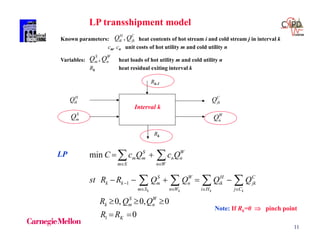
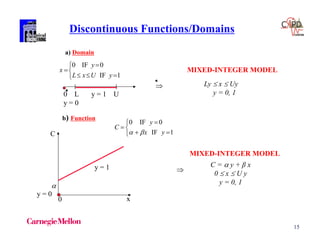
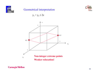
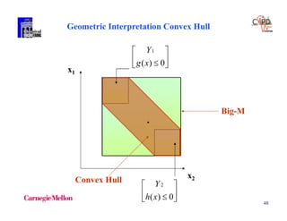
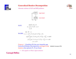
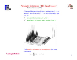
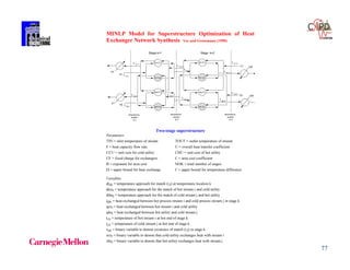
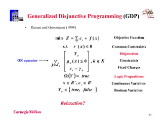
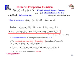
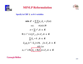
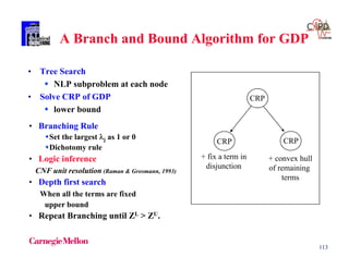
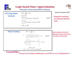
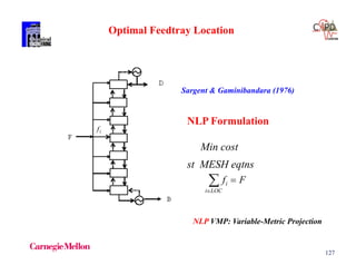
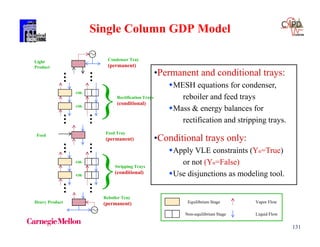
![41
EXAMPLE
Integer Cut
Constraint that is infeasible for integer point
yi = 1 i B yi = 0 i N
and feasible for all other integer points
1
1)1(
)()(
)]()[(
B
Ni
i
Bi
i
Ni
ii
Bi
i
Ni
i
Bi
i
Ni
i
Bi
yy
yy
yy
yy
Balas andJeroslow (1968)](https://image.slidesharecdn.com/shortcoursegbdminlp19alicante-190116061825/85/Mixed-integer-and-Disjunctive-Programming-Ignacio-E-Grossmann-41-320.jpg)
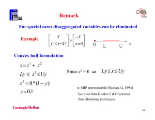
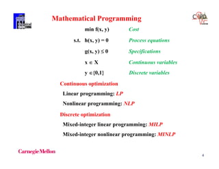
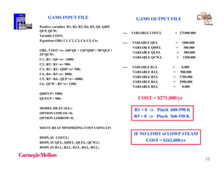
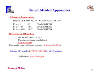
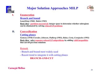
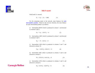
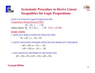
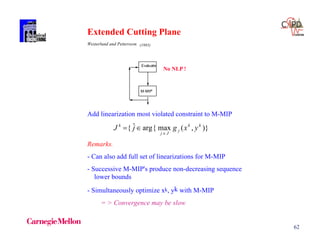
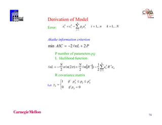
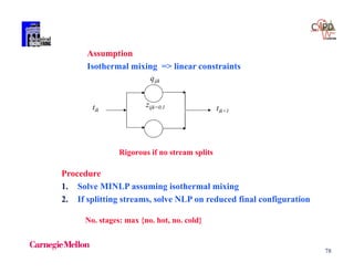
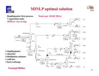
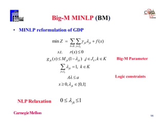
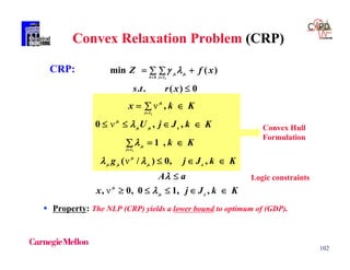
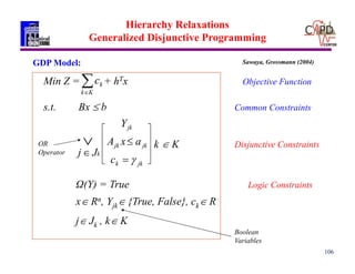
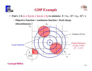
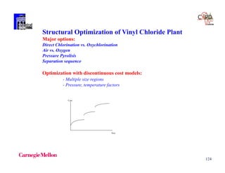
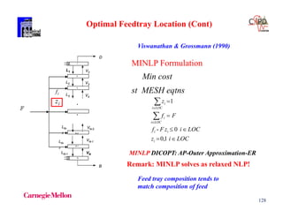
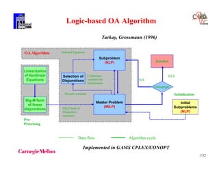
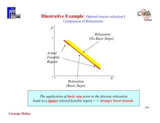
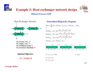
![50
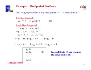
Example
[x1 – x2 - 1] [-x1 + x2 -1]
0 x1, x2 4
x2
x1
big M x1 – x2 - 1 + M (1 – y1)
-x1 + x2 - 1 + M (1 – y2)
y1 + y2 = 1 M = 10 possible choice
4
4
1
1
Convex hull
1 2
1 11
1 2
2 22
x z z
x z z
1 1 2 2
1 2 1 21 2
y yz z z z
1 2
1
1 1
2
1 2
1
2 1
2
2 2
1
0
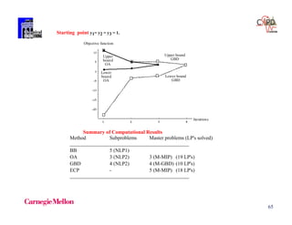
0
0
0
4
4
4
4
y y
yz
yz
yz
yz
](https://image.slidesharecdn.com/shortcoursegbdminlp19alicante-190116061825/85/Mixed-integer-and-Disjunctive-Programming-Ignacio-E-Grossmann-50-320.jpg)
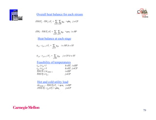
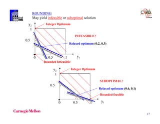
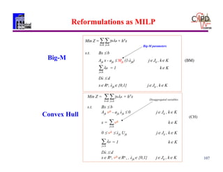
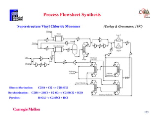
![80
Logical constraints
qijk - zijk 0iHP, jCP, kST
qcui - zcui 0 iHP
qhuj - zhuj 0 jCP
zijk, zcui, zhuj = 0,1
Calculation of approach temperatures
dtijk ti,k - tj,k + (1 - zijk) kST, iHP, jCP
dtijk+1 ti,k+1 - tj,k+1 + (1 - zijk) kST, iHP, jCP
dtcui ti,NOK+1 - TOUTCU + (1 - zcui) iHP
dthui TOUTHU - tj,1 + (1 - zhuj) jCP
dtijk EMAT
Objective function
Chen approximation (1987)
LMTD ~ [(dtl*dt2)*(dtl+dt2)/2]1/3
, ,
1/3
1 1
min
... .
[( )( )( ) / 2)]
i j
i HP j CP
ij ijk i CU i i HU j
i HP j CP k ST i HP j CP
ij ijk
i HP j CP k ST ijk ijk ijk ijk ijk
Z CCUqcu CHUqhu
CF z CF zcu CF zhu
C q
etc
U dt dt dt dt
SYNHEAT: http://newton.cheme.cmu.edu/interfaces](https://image.slidesharecdn.com/shortcoursegbdminlp19alicante-190116061825/85/Mixed-integer-and-Disjunctive-Programming-Ignacio-E-Grossmann-80-320.jpg)
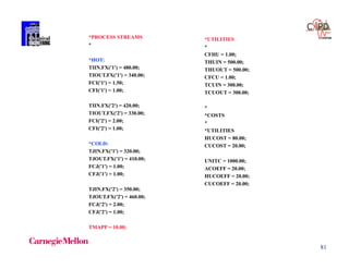
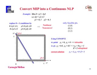
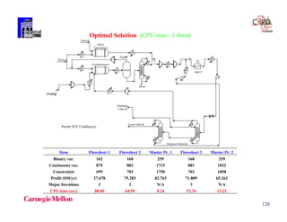
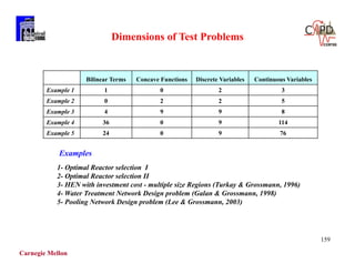
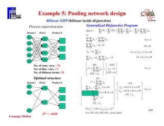
![84
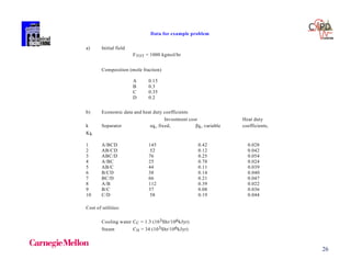
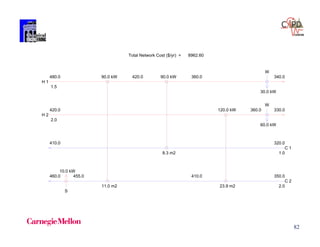
Table: Problem Data Example 2
Stream
Tin
(C)
Tout
(C)
F
( )kW C1
h
( )kW m 2 1C
Cost
($ )kW yr 1 1
H1 159 77 2.285 0.10 -
H2 267 80 0.204 0.04 -
H3 343 90 0.538 0.50 -
C1 26 127 0.933 0.01 -
C2 118 265 1.961 0.50 -
S1 300 300 - 0.05 110
W1 20 60 - 0.20 10
Cost of heat exchangers ($ yr1) = 7400 + 80 [Area(m2 )]](https://image.slidesharecdn.com/shortcoursegbdminlp19alicante-190116061825/85/Mixed-integer-and-Disjunctive-Programming-Ignacio-E-Grossmann-84-320.jpg)


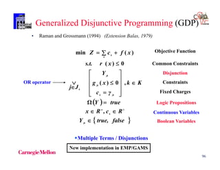
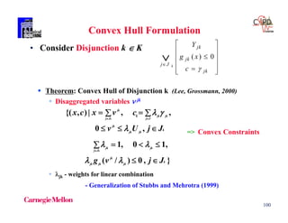
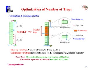
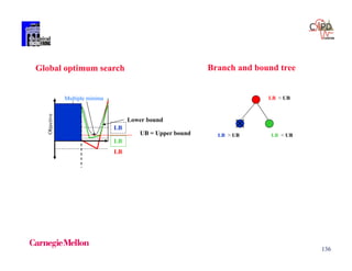
![119
• Branching Rule: j - the weight of disaggregated variable
Fix Yj as true: fix j as 1.
Y2
Root Node
Convex hull of all Si
Z = 1.154
= [0.016,0.955,0.029]
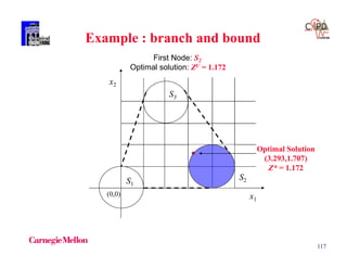
First Node
Fix 2 = 1, Z = 1.172
[x1 ,x2] = [3.293,1.707]
= [0,1,0]
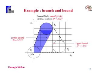
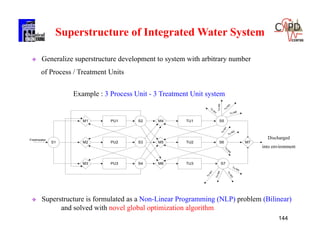
Second Node
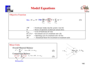
Convex hull of S1 and S3
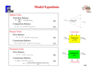
Z = 3.327
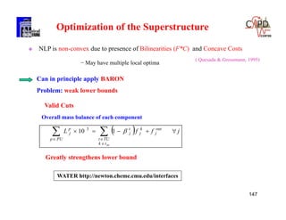
= [ 0.337,0,0.623]
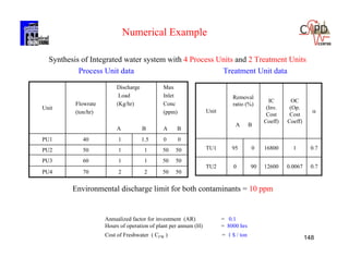
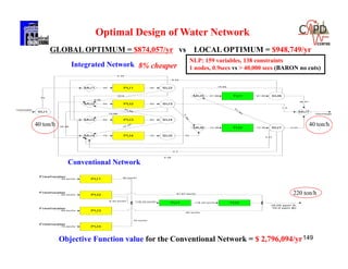
¬ Y2
ZU = 1.172
Backtrack
ZL = 1.154
Branch on Y2
ZL = 3.327 > ZU
Stop
Example: Search Tree](https://image.slidesharecdn.com/shortcoursegbdminlp19alicante-190116061825/85/Mixed-integer-and-Disjunctive-Programming-Ignacio-E-Grossmann-119-320.jpg)
![122
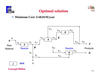
Proposed BB Method
ZL = 62.48
= [0.31,0.69,0.03,1.0,1,0,1]
ZU = 68.01 = Z*
= [0,1,0,0,1.0,1,0,1]
Optimal Solution
ZU = 71.79
= [0,1,1,1.0,1,0,1]
Feasible Solution
ZL = 75.01 > ZU
= [1,0,0.022,1.0,1,0,1]
ZL = 65.92
= [0,1,0.022,1.0,1,0,1]
0
32
41
Fix 2 = 1
Fix 3 = 1 Fix 3 = 0
Fix 2 = 0
Stop
5 nodes vs. 17 nodes of Standard BB (lower bound = 15.08)
CPU time : 2.578 vs. 3.383 of Standard BB (300MHz Pentium II PC)
Proposed BB
0
ZL = 15.08 Standard BB
1 2
43
1413 5 6
812111615 7
10*9
Y4 = 0 Y4 = 1
Y6 = 0 Y6 = 1
Y8 = 0
Y8 = 1
Y1 = 0 Y1 = 1
Y8 = 0 Y8 = 1
Y2 = 0 Y2 = 1 Y1 = 1
Y3 = 0 Y3 = 1](https://image.slidesharecdn.com/shortcoursegbdminlp19alicante-190116061825/85/Mixed-integer-and-Disjunctive-Programming-Ignacio-E-Grossmann-122-320.jpg)
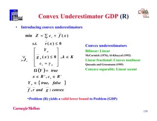
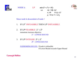
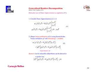
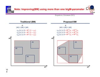
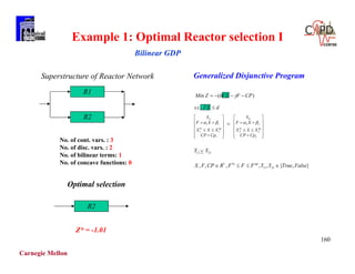
![139
Convex envelopes
Concave function
xba
Secant g(x)
[ ( ) ( )]
( ) ( ) ( )
f b f a
g x f a x a
b a
f(x)](https://image.slidesharecdn.com/shortcoursegbdminlp19alicante-190116061825/85/Mixed-integer-and-Disjunctive-Programming-Ignacio-E-Grossmann-139-320.jpg)
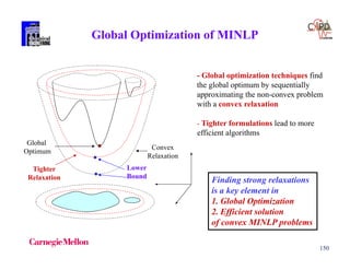
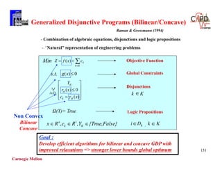


The document discusses various mathematical programming techniques, focusing on mixed-integer linear programming (MILP), mixed-integer nonlinear programming (MINLP), and generalized disjunctive programming (GDP). It highlights the challenges of developing optimal models, improving relaxations, and addressing nonconvex problem-solving. Additionally, the document illustrates several examples, optimization models, and algorithms used in this field, including the branch and bound and cutting planes methods.